Occurrence statistics of magnetic impulsive events
19
0
0
Texte intégral
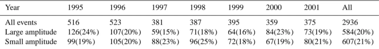
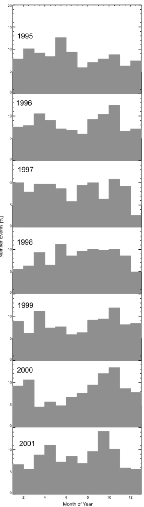
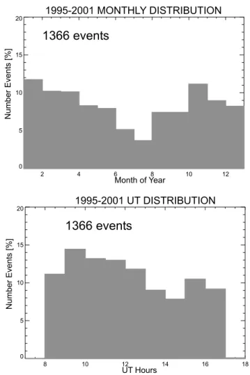
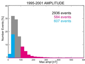
Figure


+7

Documents relatifs