HAL Id: inria-00289709
https://hal.inria.fr/inria-00289709
Submitted on 23 Jun 2008
HAL is a multi-disciplinary open access
archive for the deposit and dissemination of
sci-entific research documents, whether they are
pub-lished or not. The documents may come from
teaching and research institutions in France or
abroad, or from public or private research centers.
L’archive ouverte pluridisciplinaire HAL, est
destinée au dépôt et à la diffusion de documents
scientifiques de niveau recherche, publiés ou non,
émanant des établissements d’enseignement et de
recherche français ou étrangers, des laboratoires
publics ou privés.
Tilting at windmills with Coq: formal verification of a
compilation algorithm for parallel moves
Laurence Rideau, Bernard Serpette, Xavier Leroy
To cite this version:
Laurence Rideau, Bernard Serpette, Xavier Leroy. Tilting at windmills with Coq: formal verification
of a compilation algorithm for parallel moves. Journal of Automated Reasoning, Springer Verlag,
2008, 40 (4), pp.307-326. �10.1007/s10817-007-9096-8�. �inria-00289709�
(will be inserted by the editor)
Tilting at windmills with Coq:
formal verification of a compilation algorithm
for parallel moves
Laurence Rideau · Bernard Paul Serpette · Xavier Leroy
the date of receipt and acceptance should be inserted later
Abstract This article describes the formal verification of a compilation algorithm that transforms parallel moves (parallel assignments between variables) into a semantically-equivalent sequence of elementary moves. Two different specifications of the algorithm are given: an inductive specification and a functional one, each with its correctness proofs. A functional program can then be extracted and integrated in the Compcert verified compiler.
Keywords Parallel move · Parallel assignment · Compilation · Compiler correctness · The Coq proof assistant
1 Introduction
Parallel assignment is a programming construct found in some programming languages (Algol 68, Common Lisp) and in some compiler intermediate languages (the RTL inter-mediate language of the GNU Compiler Collection). A parallel assignment is written (x1, . . . , xn) := (e1, . . . , en), where the xi are variables and the ei are expressions
possibly involving the variables xi. The semantics of this parallel assignment is to
evaluate the expressions e1, . . . , en, then assign their respective values to the
vari-ables x1, . . . , xn. Since the left-hand side variables can occur in the right-hand side
expressions, the effect of a parallel assignment is, in general, different from that of the sequence of elementary assignments x1:= e1; . . . ; xn:= en. Welch [15] gives examples
of uses of parallel assignments.
Compiling a parallel assignment instruction amounts to finding a serialisation – a sequence of single assignments x′1 = e′1; . . . ; x′m= e′m– whose effect on the variables
xi and on other program variables is the same as that of the source-level parallel
assignment. Since parallel assignment includes permutation of variables (x1, x2) =
L. Rideau and B. P. Serpette
INRIA Sophia-Antipolis M´editerran´ee, B.P. 93, 06902 Sophia-Antipolis, France E-mail: [email protected], [email protected]
X. Leroy
INRIA Paris-Rocquencourt, B.P. 105, 78153 Le Chesnay, France E-mail: [email protected]
(x2, x1) as a special case, the generated sequence of elementary assignments cannot,
in general, operate in-place over the xi: additional storage is necessary under the form
of temporary variables. A trivial compilation algorithm, outlined by Welch [15], uses n temporaries t1, . . . , tn, not present in the original program:
t1:= e1; . . . ; tn:= en; x1:= t1; . . . ; xn:= tn
As shown by the example (x1, x2) = (x2, x1), it is possible to find more efficient
sequences that use fewer than n temporaries.
Finding such sequences is difficult in general: Sethi [14] shows that compiling a parallel assignment over n variables using at most K temporaries, where K is a constant independent of n, is an NP-hard problem. However, there exists a family of parallel assignments for which serialisation is computationally easy: parallel assignments of the form (x1, . . . , xn) := (y1, . . . , yn), where the right-hand sides yi are restricted to be
variables (either the xivariables or other variables). We call these assignments parallel
moves. They occur naturally in compilers when enforcing calling conventions [1]. May [13] shows another example of use of parallel moves in the context of machine code translation. It is a folklore result that parallel moves can be serialised using at most one temporary register, and in linear time [13].
The purpose of this paper is to formalize a compilation algorithm for parallel moves and mechanically verify its semantic correctness, using the Coq proof assistant [7, 4]. This work is part of a larger effort, the Compcert project [10, 6, 5], which aims at mechanically verifying the correctness of an optimizing compiler for a subset of the C programming language. Every pass of the Compcert compiler is specified in Coq, then proved to be semantics-preserving: the observable behavior of the generated code is identical to that of the source code.
The parallel move compilation algorithm is used in the pass that enforces calling conventions for functions. Consider a source-level function call f (e1, . . . , en). Earlier
compiler passes produces intermediate code that computes the values of the arguments e1, . . . , en and deposits them in locations l1, . . . , ln. (Locations are either processor
registers or stack slots.) The function calling conventions dictate that the separately-compiled function f expects its parameters in conventional locations l′1, . . . , l′n
de-termined by the number and types of the parameters. The register allocation phase is instructed to prefer the locations l′1, . . . , l′n for the targets of e1, . . . , en, but such
preferences cannot always be honored. Therefore, the pass that enforces calling con-ventions must, before the call, insert elementary move instructions that perform the parallel move (l′1, . . . , l′n) := (l1, . . . , ln). Only two hardware registers (one integer
reg-ister, one floating-point register) are available at this point to serve as temporaries. Therefore, the naive compilation algorithm for parallel moves will not do, and we had to implement and prove correct the space-efficient algorithm.
The formal specification and correctness proof of this compilation algorithm is chal-lenging. Indeed, this was one of the most difficult parts of the whole Compcert devel-opment. While short and conceptually clear, the algorithm we started with (described section 3) is very imperative in nature. The underlying graph-like data structure, called windmills in this paper, is unusual. Finally, the algorithm involves non-structural re-cursion. We show how to tackle these difficulties by progressive refinement from a high-level, nondeterministic, relational specification of semantics-preserving transfor-mations over windmills.
The remainder of this paper is organized as follows. Section 2 defines the wind-mill structure. Section 3 shows the folklore, imperative serialisation algorithm that we
used as a starting point. Two inductive specifications of the algorithm follow, a non-deterministic one (section 4), and a non-deterministic one (section 5), with the proofs that they are correct and consistent. Section 6 derives a functional implementation from these specifications and proves consistency with the inductive specifications, termina-tion, and correctness. Section 7 proves additional syntactic properties of the result of the compilation function. In section 8, the correctness result of section 6 is extended to the case where variables can partially overlap. Concluding remarks are presented in section 9.
The complete, commented source for the Coq development presented here is avail-able at http://gallium.inria.fr/~xleroy/parallel-move/.
2 Definitions and notations
An elementary move is written (s 7→ d), where the source register s and the destination register d range over a given set R of registers. Parallel moves as well as sequences of elementary moves are written as lists of moves (s17→ d1) · · · (sn7→ dn). The · operator
denotes the concatenation of two lists. We overload it to also denote prepending a move in front of a list, (s 7→ d) · l, and appending a move at the end of a list, l · (s 7→ d). The empty list is written ∅.
We assume given a set T ⊆ R of temporary registers: registers that are not men-tioned in the initial parallel move problem and that the compiler can use to break cycles. We also assume given a function T : R → T that associates to any register r a temporary register T (r) appropriate for saving the value of r when breaking a cycle involving r. In the simplest case, only one temporary tmp is available and T is the con-stant function T (r) = tmp. In more realistic cases, architectural or typing constraints may demand the use of several temporaries, for instance one integer temporary to move integer or pointer values, and one floating-point temporary to move floating-point val-ues. In this example, T (r) selects the appropriate temporary as a function of the type of r.
A parallel move (s1 7→ d1) · · · (sn 7→ dn) is well defined only if the destination
registers are pairwise distinct: di 6= dj if i 6= j. (If a register appeared twice as a
destination, its final value after the parallel move would not be uniquely defined.) We call such parallel moves windmills.
Definition 1 (Windmills) A parallel move µ is a windmill if, for all l1, si, di, l2, sj,
dj and l3,
µ = l1· (si7→ di) · l2· (sj7→ dj) · l3 ⇒ di6= dj
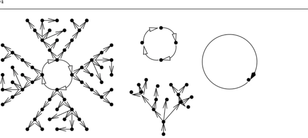
The name “windmill” comes from the graphical shape of the corresponding transfer relation. We can view a parallel move as a transfer relation. Each move (si 7→ di)
corresponds to an edge in the graph of this relation. A parallel move is a windmill if every register has at most one predecessor for the transfer relation. Although this property is similar to the specification of forests (set of disjoint trees), it allows cycles such as (r17→ r2) · (r27→ r1). This is unlike a tree, where, by definition, there exists a
unique element – the root – that has no predecessor.
The graph of the relation corresponding to a windmill is composed of cycles – the axles – whose elements are the roots of trees – the blades. Figure 1 figure shows a set of 4 windmills: the general case, the special case of a tree, a simple cycle with four registers, and the special case of a self-loop.
Fig. 1 Examples of windmills
3 An imperative algorithm
There are two special cases of parallel move problems where serialization is straightfor-ward. In the case of a simple cycle, i.e. an axle without any blade, the transfer relation is:
(r17→ r2) · (r27→ r3) · · · (rn−17→ rn) · (rn7→ r1)
Serialization is done using a single temporary register t = T (r1):
t := r1; r1:= rn; rn:= rn−1; . . . ; r3:= r2; r2:= t.
The other easy case corresponds to a transfer relation that is a tree, such as for instance
(r17→ r2) · (r17→ r3) · (r27→ r4)
In this case, serialization corresponds to enumerating the edges in a bottom-up topo-logical order:
r4:= r2; r2:= r1; r3:= r1.
C. May [13] describes an algorithm that generalizes these two special cases. This al-gorithm follows the topology of the transfer relation. First, remove one by one all the edges that have no successors, emitting the corresponding sequential assignments in the same order. (In windmill terminology, this causes the blades to disappear little by little.) Eventually, all that remains are simple, disjoint cycles (windmill axles) which can be serialized using one temporary as described above.
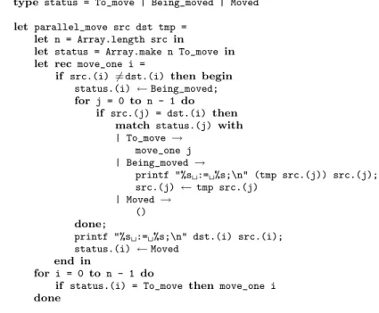
We now consider a variant of this algorithm that processes blades and axles simul-taneously, in a single pass. The algorithm is given in figure 2 in Caml syntax [11]. It can be read as pseudo-code knowing that a.(i) refers to the i-th element of array a. It takes as arguments two arrays src and dst containing respectively the source reg-isters s1, . . . , snand the target registers d1, . . . , dn, as well as the temporary-generating
function tmp. The elementary moves produced by serialization are successively printed using the C-like printf function.
The algorithm implements a kind of depth-first graph traversal using the move_one function that takes an edge (srci 7→ dsti) of the transfer relation as an argument. In
line 9 and 10, all successors of dsti are handled. Line 17 handles the case of an already
analysed edge. In the case of line 12, it is a simple recursive call. In the case of line 14, a cycle is discovered and a temporary register is used to break it.
1 type status = To_move | Being_moved | Moved 2
3 let parallel_move src dst tmp = 4 let n = Array.length src in
5 let status = Array.make n To_move in 6 let rec move_one i =
7 if src.(i) 6= dst.(i) then begin 8 status.(i) ← Being_moved; 9 for j = 0 to n - 1 do 10 if src.(j) = dst.(i) then 11 match status.(j) with
12 | To_move → 13 move_one j 14 | Being_moved → 15 printf "%sÃ:=Ã%s;\n" (tmp src.(j)) src.(j); 16 src.(j) ← tmp src.(j) 17 | Moved → 18 () 19 done;
20 printf "%sÃ:=Ã%s;\n" dst.(i) src.(i); 21 status.(i) ← Moved
22 end in
23 for i = 0 to n - 1 do
24 if status.(i) = To_move then move_one i 25 done
Fig. 2 A one-pass, imperative algorithm to compile parallel moves
When exiting this loop on line 19, all the nodes that can be reached by dsti have
been analysed, the edge (srci7→ dsti) is serialized and marked as analyzed.
When a cycle is discovered, the stack of active calls to move_one correspond to the edges ((rn 7→ r1), . . . , (r2 7→ r3), (r1 7→ r2)) and, at line 14, the edge (r1 7→ r2) is
analysed again. The side effect of line 16 thus necessarily acts on the edge that started the recursion of the move_one function, i.e. the edge at the bottom of the stack. The main loop, lines 23 to 25, ensures that all edges are analyzed at least once.
4 Nondeterministic specification
The algorithm in figure 2 does not lend itself easily to program proof: first, it is writ-ten imperatively, making it quite removed from a mathematical specification; second, it commits to a particular strategy for solving the problem, obscuring the essential invariants for the correctness proof. In this section, we develop an abstract specifica-tion of the steps of the algorithm, and show that these steps preserve semantics. This specification is not deterministic: it does not constrain which step must be taken in a given state.
In the algorithm of figure 2, notice that every edge of the transfer relation begins in the state To_move (line 5), then takes the state Being_moved (line 8), and finally reaches the state Moved (line 21). Rather than associating a status to each edge, we will represent the current state of the compilation as three disjoint lists of edges, each list containing edges having the same status. The state is therefore a triple (µ, σ, τ ) of lists of edges: µ is the to-move list, σ the being-moved list and τ the moved list.
Each step of the algorithm will either extract an element from the to-move list µ and add it to the being-moved list σ, or remove an element of the latter and add it to the moved list τ . The to-move and being-moved lists are used as work lists; the algorithm will stop when both are empty.
The being-moved list σ is used as a stack, simulating the recursive calls to the move_one function in the imperative algorithm. In addition to pushing and popping moves from the beginning of σ, the last element of σ can also be modified when a cycle is discovered.
The last component of the state, the moved list τ , is used to accumulate the sequence of elementary moves that the imperative algorithm emits using the printf function. Moves are successively added to the front of the list τ . Therefore, the elementary moves listed in τ are to be executed from right to left.
4.1 Inference rules
The inference rules below define a rewriting relation ⊲ between states (µ, σ, τ ). Each rule describes a step that the compilation algorithm is allowed to take. A run of compilation is viewed as a sequence of rewrites from the initial state (µ, ∅, ∅) to a final state (∅, ∅, τ ), where µ is the parallel move problem we set out to compile, and reverse(τ ) is the sequence of elementary moves generated by this compilation run.
(µ1· (r 7→ r) · µ2, σ, τ ) ⊲ (µ1· µ2, σ, τ )
[Nop]
The first rule deals with the case where the transfer relation has an edge (r 7→ r) whose source and destination are identical. This case is specially handled at line 7 of the imperative algorithm. Note that in the imperative algorithm, this edge is not annotated as Moved and keeps the status To_move until the end of the algorithm. Nevertheless this edge cannot result from a recursive call of the function move_one because, in this case, the caller would correspond to an edge (s 7→ r) and that would violate the fact that the transfer relation is a windmill: indeed, there would exist two different edges with the same destination. It is therefore valid to move the test of line 7 up to the level of the main loop at line 24.
(µ1· (s 7→ d) · µ2, ∅, τ ) ⊲ (µ1· µ2, (s 7→ d), τ )
[Start]
The [Start] rule corresponds to the first call to the move_one function at line 24. We know that in this case no edge has the status Being_Moved and this rule will thus be the only one to handle the case where the being-moved list is empty.
(µ1· (d 7→ r) · µ2, (s 7→ d) · σ, τ )
⊲ (µ1· µ2, (d 7→ r) · (s 7→ d) · σ, τ )
[Push]
The [Push] rule corresponds to the recursive call at line 13. If the edge being analysed is (s 7→ d) (i.e. the top of the being-moved list) and if there exists a successor (d 7→ r) in the to-move list, the latter is transferred to to the top of the being-moved stack.
The [Loop] rule corresponds to the special case at lines 15 and 16 where a cycle is discovered. This rule is of more general use. Indeed, it is not essential to check the presence of a cycle before inserting a transfer using a temporary register. Thus, lines 15 and 16 can also be moved up to the level of the main loop (line 24). The fact that one uses the temporary register only in the case of a cycle must be regarded as an optimization. The crucial issue is to make sure that a transfer through a temporary register must be used whenever a cycle arises. This is ensured by the next rule.
NoRead(µ, dn) ∧ dn6= s0
(µ, (sn7→ dn) · σ · (s07→ d0), τ )
⊲ (µ, σ · (s07→ d0), (sn7→ dn) · τ )
[Pop]
The [Pop] rule corresponds to returning from a recursive call to the function move_one. The first premise of this rule, NoRead(µ, dn), is formally defined as
NoRead(µ, dn) def
= ∀µ1, s, µ2, µ = µ1· (s 7→ d) · µ2 ⇒ s 6= dn.
This premise checks that the edge (sn7→ dn) under study no longer has its successor
dn in the to-move list. It therefore prevents the [Pop] rule from being used if the value
of dn is still needed. The second premise, dn 6= s0, makes sure that the [Pop] rule
cannot be used if dn participates in a cycle, forcing the use of the [Loop] rule instead
in the case of a cycle.
NoRead(µ, dn)
(µ, (s 7→ d), τ ) ⊲ (µ, ∅, (s 7→ d) · τ ) [Last]
The [Last] rule corresponds to returning from the main loop at line 24. It is a special case of the [Pop] rule. As in the special case of the [Nop] rule, observe that a to-move list of the form ((r 7→ r)) can either be eliminated by the [Nop] rule, or rewritten to itself in two steps ([Start] then [Last]), or rewritten to ((T (r) 7→ r) · (r 7→ T (r))) using a temporary register (rules [Start] then [Loop] then [Last]). These three results are equally valid.
4.2 Well-formedness invariant
In preparation for proving the semantic correctness of the rewriting rules, we first define a well-formedness property that acts as a crucial invariant in this proof.
Definition 2 (Invariant) A triple (µ, σ, τ ) is well-formed, written ⊢ (µ, σ, τ ), if and only if:
1. µ · σ is a windmill, in the sense of definition 1.
2. The µ list does not contain temporary registers: for all µ1, s, d, µ2,
µ = µ1· (s 7→ d) · µ2 ⇒ (s /∈ T ∧ d /∈ T ).
3. The σ list can only use a temporary register as the source of its last edge: for all σ1, s0, d0,
σ = σ1· (s07→ d0) ⇒ d0∈ T/
and for all σ2, s, d, σ3,
4. The σ list is a path: σ = (rn−17→ rn) · · · (r27→ r3) · (r17→ r2) for some registers
r1, . . . , rn.
Notice that if µ is a windmill and does not use any temporary register, then the initial triple (µ, ∅, ∅) is well-formed.
Lemma 1 (The invariant is preserved) The rewriting rules transform a well-formed triple into a well-well-formed triple. If S1⊲ S2and⊢ S1, then⊢ S2.
Proof By case analysis on the rule that concludes S1⊲ S2. For S1= (µ, σ, τ ), only the
[Push] rule adds an element to σ, but the edge thus added extends the path already present in σ.
4.3 Dynamic semantics for assignments
To state semantic preservation for the rewriting relation, we need to give dynamic semantics to the parallel moves µ and the sequential moves σ and τ occurring in intermediate states. Let V be the set of run-time values for the language. The run-time state of a program is represented as an environment ρ : R → V mapping registers to their current values. Assigning value v to register r transforms the environment ρ into the environment ρ[r ← v] defined by
ρ[r ← v] =nr 7→ vr′
7→ ρ(r′) if r′6= r.
(We assume that assigning to a register r preserves the values of all other registers r′, or in other words that r does not overlap with any other register. We will revisit this hypothesis in section 8.)
The run-time effect of a parallel move µ is to transform the current environment ρ in the environment [[µ]]//(ρ) defined as:
[[(sn7→ dn) · · · (s07→ d0)]]//(ρ) = ρ[d0← ρ(s0)] . . . [dn← ρ(sn)]
In this definition parentheses are omitted, as we require that µ is a windmill. The fol-lowing lemma, showing that the order of moves within µ does not matter, is intensively used in our proofs:
Lemma 2 (Independence) If µ = µ1· (s 7→ d) · µ2is a windmill, then
[[µ]]//(ρ) = [[(s 7→ d) · µ1· µ2]]//(ρ)
Proof By induction on µ1. The base case µ1= ∅ is trivial. For the inductive step, we
need to prove that the first two elements of µ1can be exchanged: (ρ[d0← ρ(s0)])[d1←
ρ(s1)] = (ρ[d1 ← ρ(s1)])[d0 ← ρ(s0)]. The windmill structure of µ1 implies that
d06= d1, and therefore this equality is verified.
The run-time effect of a sequence of elementary moves τ , performed from left to right, is defined by:
[[∅]]→(ρ) = ρ
The sequences of elementary moves τ appearing in the states of the rewriting rela-tion are actually to be interpreted from right to left, or equivalently to be reversed before execution. It is therefore useful to define directly the semantics of a sequence of elementary moves τ performed from right to left:
[[∅]]←(ρ) = ρ
[[(s 7→ d) · τ ]]←(ρ) = ρ′[d ← ρ′(s)] where ρ′= [[τ ]]←(ρ)
Lemma 3 (Reversed sequential execution) For all sequences τ of elementary moves, [[τ ]]←(ρ) = [[reverse(τ )]]→(ρ).
Proof Easy induction over τ .
Definition 3 (Equivalent environments) We say that two environments ρ1 and
ρ2are equivalent, and we write ρ1≡ ρ2, if and only if all non-temporary registers have
the same values in both environments:
ρ1≡ ρ2 def
= ∀r /∈ T , ρ1(r) = ρ2(r).
Definition 4 (Semantics of a triple) The dynamic semantics of the triple (µ, σ, τ ) corresponds to first executing τ sequentially from right to left, then executing µ · σ in parallel:
[[(µ, σ, τ )]](ρ) = [[µ · σ]]//([[τ ]]←(ρ)).
Notice that for initial states, we have [[(µ, ∅, ∅)]](ρ) = [[µ]]//(ρ), while for final states, we have [[(∅, ∅, τ )]](ρ) = [[τ ]]←(ρ) = [[reverse(τ )]]→(ρ).
4.4 Correctness
Lemma 4 (One-step semantic preservation) The rewriting rules preserve the se-mantics of well-formed triples: if S1 ⊲ S2 and ⊢ S1, then [[S1]](ρ) ≡ [[S2]](ρ) for all
environments ρ.
Proof By case analysis on the rule used to derive S1⊲ S2. We write S1= (µ, σ, τ ).
– Rule [Nop]: use the fact that ρ[r ← ρ(r)] = ρ.
– Rules [Start] and [Push]: use the order independence lemma 2.
– Rule [Loop]: exploit the fact that µ and σ do not use the temporary register intro-duced by the rule.
– Rule [Pop]: the expected result follows from
[[(sn7→ dn) · µ · σ]]//([[τ ]]←(ρ)) = [[µ · σ]]//([[(sn7→ dn) · τ ]]←(ρ))
This equality holds provided that register dn does not appear as a source in µ · σ.
For µ, this is ensured by the first premise. For σ, this follows by induction from the fact that σ is a path. The base case comes from the premise dn6= s0. The inductive
case is provided by the windmill structure of σ. – Rule [Last]: special case of rule [Pop].
Lemma 5 (Semantic preservation) Several steps of rewriting preserve the seman-tics of well-formed triples: if S1⊲∗S2 and⊢ S1, then [[S1]](ρ) ≡ [[S2]](ρ) for all
envi-ronments ρ.
Proof By induction on the number of steps.
As a corollary, we obtain the main semantic preservation theorem of this section.
Theorem 1 (Correctness of ⊲∗) If µ is a windmill containing no temporary register, and if the triple (µ, ∅, ∅) can be rewritten into (∅, ∅, τ ) then the parallel execution of µ is equivalent to the sequential execution of reverse(τ ):
(µ, ∅, ∅) ⊲∗(∅, ∅, τ ) ⇒ [[µ]]//(ρ) ≡ [[reverse(τ )]]→(ρ).
5 Deterministic specification
The next step towards an effective algorithm consist in determinising the inductive rules of section 4 by ensuring that at most one rule matches a given state, and by specifying which edge to extract out of the to-move list in the rules [Nop], [Push] and [Start]. ((r 7→ r) · µ, ∅, τ ) ֒→ (µ, ∅, τ ) [Nop ′] s 6= d ((s 7→ d) · µ, ∅, τ ) ֒→ (µ, (s 7→ d), τ ) [Start ′]
The first two rules treat the case of an empty being-moved list and consider only the first element on the left of the to-move list µ.
NoRead(µ1, d)
(µ1· (d 7→ r) · µ2, (s 7→ d) · σ, τ )
֒→ (µ1· µ2, (d 7→ r) · (s 7→ d) · σ, τ )
[Push′]
The [Push′] rule treats the case in which the analysed edge has a successor in the µ list. It forces the algorithm to consider the leftmost successor found in µ.
NoRead(µ, r0) (µ, (s 7→ r0) · σ · (r07→ d), τ ) ֒→ (µ, σ · (T (r0) 7→ d), (s 7→ r0) · (r07→ T (r0)) · τ ) [LoopPop] NoRead(µ, dn) ∧ dn6= s0 (µ, (sn7→ dn) · σ · (s07→ d0), τ ) ֒→ (µ, σ · (s07→ d0), (sn7→ dn) · τ ) [Pop′]
These two rules treat the case where the analysed edge has no successor in the to-move list, and the being-to-moved list contains at least two elements. The [LoopPop] rule is the [Pop] rule in the case of a cycle. This rule, unlike the corresponding nondeterministic rules, pops the analysed edge. This ensures that every rule moves at least one edge. The termination proof in section 6 uses this fact.
NoRead(µ, d)
(µ, (s 7→ d), τ ) ֒→ (µ, ∅, (s 7→ d) · τ ) [Last
′]
The [Last′] rule treats the final case where the being-moved list contains only one element.
Since these deterministic rules are instances or combinations of the nondeterministic ones, the following two lemmas are trivial.
Lemma 6 (Inclusion ֒→ ⊆⊲∗) If S1֒→ S2, then S1⊲∗S2.
Proof By case analysis. The [LoopPop] case uses the transitivity of ⊲∗.
Lemma 7 (Inclusion ֒→∗ ⊆⊲∗) If S1֒→∗S2, then S1⊲∗S2.
Proof By induction on the number of steps.
Notice that the deterministic rules implement a strategy that is slightly different from that of the imperative algorithm. Indeed, during the imperative algorithm, when a temporary register is used to break a cycle, the analysed edge can still have a successor. This is not the case for the [LoopPop] rule.
Semantic preservation for the deterministic rules follows immediately from theo-rem 1 and lemma 7. However, to obtain an algorithm, we still need to prove that the rules are indeed deterministic and that a normal form (i.e. the final state (∅, ∅, τ )) always exists. To do so, we now give a functional presentation of the deterministic rules.
6 The functional algorithm
From the deterministic rules in section 5, it is easy to build a function stepf that performs one step of rewriting. Compiling a parallel move problem, then, corresponds to iterating stepf until a final state is reached:
pmov S =
match S with | (∅ , ∅ , _) ⇒ S | _ ⇒ pmov (stepf S) end
However, such a function definition is not accepted by Coq, because it is not structurally recursive: the recursive call is performed on stepf(S) and not on a structural subterm of S. To define the pmov function, we will use the Coq command Function, which provides a simple mechanism to define a recursive function by well-founded recursion [2, 3]. To this end, we first define the stepf function that executes one computation step, then a measure function which will be used to justify termination, and finally the theorem establishing that the measure decreases at each recursive call.
Function stepf (st: state) : state := match st with
| State ∅ ∅ _ ⇒ st (∗ final state ∗) | State ((s, d) · tl) ∅ l ⇒
if reg_eq s d
then State tl ∅ l (∗ s = d; rule [Nop] ∗) else State tl ((s, d) · ∅ ) l (∗ s 6= d; rule [ Start ] ∗) | State t ((s, d) · b) l ⇒
match split_move t d with
| Some (t1, r, t2) ⇒ (∗ t = t1· (d 7→ r) · t2 ∗)
State (t1 · t2) (∗ rule [Push] ∗) ((d, r) · (s, d) · b)
l | None ⇒
match b with
| ∅ ⇒ State t ∅ ((s, d) · l) (∗ rule [Last] ∗) | _ ⇒
if is_last_source d b (∗ check if b = · (d 7→ ) ∗) then State t (∗ rule [LoopPop] ∗)
(replace_last_source (temp d) b) ((s, d) · (d, temp d) · l)
else State t b ((s, d) · l) (∗ rule [Pop] ∗) end
end end.
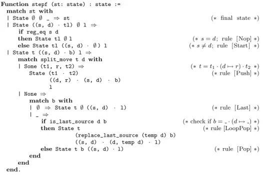
Fig. 3 The one-step rewriting function
6.1 The one-step rewriting function
We define the one-step rewriting function stepf in a way that closely follows the deterministic rules of section 5. It takes a state S as argument and returns a state S′ such that S ֒→ S′. The function, written in Coq syntax, is defined by case analysis in figure 3.
The first case (line 3) does not correspond to any of the inductive rules: it detects a final state (∅, ∅, τ ) and returns it unchanged. The other cases correspond to the deterministic rules indicated in comments.
The reg eq function decides whether two registers are equal or not. The split move function takes as arguments a windmill t and a register d. If this register is the source of an edge from list t, the function returns this edge (d, ) and the two remaining sub-lists. This breaks the t list into t1· (d, r) · t2like the [Push] rule does.
Finally, the replace last source function takes as argument a list b of edges and a register r, and replaces the source of the last edge of b with r: hb · (s 7→ d) becomes hb · (t 7→ d), in accordance with the [LoopPop] rule.
Since the definition of the stepf function is close to the deterministic specification, the following theorem is easily proved:
Lemma 8 ( Compatibility of stepf and ֒→) S ֒→ stepf(S) if S is not a final state (i.e. not of the form (∅, ∅, τ )).
Proof By case analysis on the shape of S and application of the corresponding rules for the ֒→ relation.
6.2 The general recursive function
The general recursive function consists in iterating the stepf function. To ensure ter-mination of this function, we need a nonnegative integer measure over states that de-creases at each call to the stepf function, except in the final case (∅, ∅, τ ). Examination of the deterministic rewriting rules and of the lengths of the to-move and being-moved lists reveals that:
– either an edge is removed from the to-move list and and the being-moved list is unchanged (rule [Nop]);
– or an edge is transferred from the to-move list to the being-moved list (rules [Start] and [Push]);
– or the to-move list remains the same while an edge is transferred from the being-moved list to the being-moved list (rules [LoopPop], [Pop], and [Last]).
Therefore, either one of the to-move or being-moved lists loses one element, or one element is transferred from the former to the latter. Decrease is achieved by giving more weight to the to-move edges, as the following meas function does:
Definition 5 (The triple measure) meas(µ, σ, τ ) = 2 × length(µ) + length(σ).
Lemma 9 (Measure decreases with ֒→) If S1֒→ S2, then meas(S2) < meas(S1).
Proof By case analysis on the rules of the ֒→ relation and computation of the corre-sponding measures.
Combining this lemma with lemma 8 (compatibility of stepf with ֒→), we obtain: Lemma 10 (Measure decreases with stepf) If S is not a final state, i.e. not of the form (∅, ∅, τ ), then meas(stepf(S)) < meas(S).
We can then define the iterate of stepf using the Function command of Coq version 8:
Function pmov (S: State) {measure meas st} : state := if final_state S then S else pmov (stepf S).
where final state is a boolean-valued function returning true if its argument is of the form (∅, ∅, τ ) and false otherwise. Coq produces a proof obligation requiring the user to show that the recursive call to pmov is actually decreasing with respect to the meas function. This obligation is trivially proved by lemma 10. Coq then generates and automatically proves the following functional induction principle that enables us to reason over the pmov function:
(∀S, final state(S) = true ⇒ P (S, S)) ∧ (∀S, final state(S) = false
∧ P (stepf(S), pmov(stepf(S))) ⇒ P (S, pmov(stepf(S))) ⇒ (∀S, P (S, pmov(S)))
Using this induction principle and lemma 8, we obtain the correctness of pmov with respect to the deterministic specification.
Lemma 11 For all initial states S, pmov(S) is a final state (∅, ∅, τ ) such that S ֒→∗ (∅, ∅, τ ).
6.3 The compilation function
To finish this development, we define the main compilation function, taking a parallel move problem as input and returning an equivalent sequence of elementary moves. Definition parmove (mu: moves) : moves :=
match pmov (State mu ∅ ∅ ) with | State _ _ tau ⇒ reverse tau end.
The semantic correctness of parmove follows from the previous results.
Theorem 2 Let µ be a parallel move problem. If µ is a windmill and does not mention temporary registers, then [[parmove(µ)]]→(ρ) ≡ [[µ]]//(ρ) for all environments ρ.
Proof By definition of parmove and lemma 11, we have parmove(µ) = reverse(τ ) and (µ, ∅, ∅) ֒→∗(∅, ∅, τ ). By lemma 7, this entails (µ, ∅, ∅) ⊲∗ (∅, ∅, τ ). The result follows
from theorem 1.
Here is an alternate formulation of this theorem that can be more convenient to use.
Theorem 3 Let µ = (s17→ d1) · · · (sn7→ dn) be a parallel move problem. Assume that
the di are pairwise distinct, and that si∈ T and d/ i∈ T for all i. Let τ = parmove(µ)./
For all initial environments ρ, the environment ρ′= [[τ ]]→(ρ) after executing τ
sequen-tially is such that
1. ρ′(di) = ρ(si) for all i = 1, . . . , n;
2. ρ′(r) = ρ(r) for all registers r /∈ {d
1, . . . , dn} ∪ T .
Proof By theorem 2, we know that ρ′ ≡ [[µ]]//(ρ). For (1), since di ∈ T , we have/
ρ′(di) = [[µ]]//(ρ)(di) = ρ(si) by lemma 2. For (2), we have ρ′(r) = [[µ]]//(ρ)(r), and
an easy induction on µ shows that [[µ]]//(ρ)(r) = ρ(r) for all registers r that are not destinations of µ.
Finally, we used the Coq extraction mechanism [12] to automatically generate exe-cutable Caml code from the definition of the parmove function, thus obtaining a verified implementation of the parallel move compilation algorithm that can be integrated in the Compcert compiler back-end.
7 Syntactic properties of the compilation algorithm
In this section, we show a useful syntactic property of the sequences of moves generated by the parmove compilation function: the registers involved in the generated moves are not arbitrary, but either appear in the initial parallel move problem, or are results of the temporary-generating function T .
More formally, let µ0 = (s1 7→ d1) · · · (sn 7→ dn) be the initial parallel move
problem. We define a property P (s 7→ d) of elementary moves (s 7→ d) by the following inference rules: (s 7→ d) ∈ µ0 P (s 7→ d) P (s 7→ d) P (T (s) 7→ d) P (s 7→ d) P (s 7→ T (s))
We extend this property pointwise to lists l of moves and to states:
P (l) def= ∀(s 7→ d) ∈ l, P (s 7→ d) P (µ, σ, τ ) def= P (µ) ∧ P (σ) ∧ P (τ )
Obviously, the property P holds for µ0 and therefore for the initial state (µ0, ∅, ∅).
Moreover, the property is preserved by every rewriting step.
Lemma 12 If S1⊲ S2and P (S1) hold, then P (S2) holds.
Proof By examination of the nondeterministic rewriting rules. The result is obvious for all rules except [Loop], since these rules do not generate any new moves. The [Loop] rule replaces a move (s 7→ d) that satisfies P with the two moves (T (s) 7→ d) and (s 7→ T (s)). The new moves satisfy P by application of the second and third inference rules defining P .
It follows that the result of parmove(µ0) satisfies property P .
Lemma 13 For all moves (s 7→ d) ∈ parmove(µ0), the property P (s 7→ d) holds.
Proof Follows from lemmas 7, 11 and 12.
As a first use of this lemma, we can show that for every move in the generated sequence parmove(µ0), the source of this move is either a source of µ0or a temporary,
and similarly for the destination.
Lemma 14 For all moves (s 7→ d) ∈ parmove(µ0), we have s ∈ {s1, . . . , sn} ∪ T and
d ∈ {d1, . . . , dn} ∪ T .
Proof We show that P (s 7→ d) implies s ∈ {s1, . . . , sn} ∪ T and d ∈ {d1, . . . , dn} ∪ T
by induction on a derivation of P (s 7→ d), then conclude with lemma 13.
Another application of lemma 13 is to show that the compilation of parallel moves preserves register classes. Most processors divide their register set in several classes, e.g. a class of scalar registers and a class of floating-point registers. Instructions are provided to perform a register-to-register move within the same class, but moves between two register of different classes are not supported. Assume that every register r has an associated class Γ (r). We say that a list of moves l respects register classes if Γ (s) = Γ (d) for all (s 7→ d) ∈ l.
Lemma 15 (Register class preservation) Assume that temporaries are generated in a class-preserving manner: Γ (T (s)) = Γ (s) for all registers s. If µ0 respects register
classes, then parmove(µ0) respects register classes as well.
Proof We show that P (s 7→ d) implies Γ (s) = Γ (d) by induction on a derivation of P (s 7→ d), then conclude using lemma 13.
8 Extension to overlapping registers
So far, we have assumed that two distinct registers never overlap: assigning one does not change the value of the other. This is not always the case in practice. For instance, some processor architectures expose hardware registers that share some of their bits. In the IA32 architecture, for example, the register AL refers to the low 8 bits of the 32-bit register EAX. Assigning to AL therefore modifies the value of EAX, and conversely. Overlap also occurs naturally when the “registers” manipulated by the parallel move compilation algorithm include memory locations, such as variables that have been spilled to memory during register allocation, or stack locations used for parameter passing. For example, writing a 32-bit integer at offset δ in the stack also changes the values of the stack locations at offsets δ + 1, δ + 2 and δ + 3.
It is not straightforward to generalize the parallel move compilation algorithm to the case where source and destination registers can overlap arbitrarily. We will not attempt to do so in this section, but set out to show a weaker, but still useful result: the unmodified parallel move algorithm produces correct sequences of elementary as-signments even if registers can in general overlap, provided destinations and sources do not overlap.
8.1 Formalising overlap
In the non-overlapping case, two registers r1 and r2 are either identical r1 = r2 or
different r16= r2. When registers can overlap, we have three cases: r1and r2are either
identical (r1 = r2) or completely disjoint (written r1 ⊥ r2) or different but partially
overlapping (written r1⊲⊳ r2).
We assume given a disjointness relation ⊥ over R × R, which must be symmetric and such that r1 ⊥ r2 ⇒ r1 6= r2. We define partial overlap r1 ⊲⊳ r2 as (r1 6=
r2) ∧ ¬(r1⊥ r2).
In the non-overlapping case, the semantics of an assignment of value v to register r is captured by the update operation ρ[r ← v], characterized by the “good variable” property:
ρ[r ← v] =nr 7→ vr′7→ ρ(r′) if r′6= r.
To account for the possibility of overlap, we define the weak update operation ρ[r ⇐ v] by the following “weak good variable” property:
ρ[r ⇐ v] =
(r 7→ v
r′7→ ρ(r′) if r′⊥ r r′7→ undefined if r′⊲⊳ r.
As suggested by the fatter arrow ⇐, weak update sets the target register r to the specified value v, but causes “collateral damage” on registers r′ that partially overlap
with r: their values after the update are undefined. Only registers r′ that are disjoint from r keep their old values.
Using weak update instead of update, the semantics of a sequence τ of elementary moves becomes
[[∅]]⇒(ρ) = ρ
8.2 Effect of overlap on the parallel move algorithm
In this section, we consider a parallel move problem µ = (s17→ d1) · · · (sn 7→ dn) and
assume that the sources s1, . . . , snand the destinations d1, . . . , dnsatisfy the following
hypotheses:
1. No temporaries: si⊥ t and di⊥ t for all i, j and t ∈ T .
2. Destinations are pairwise disjoint: di⊥ dj if i 6= j.
3. Sources and destinations do not partially overlap: si6= dj ⇒ si⊥ dj for all i, j.
4. Distinct temporaries do not partially overlap: t16= t2 ⇒ t1⊥ t2for all t1, t2∈ T .
As we show below, these hypotheses ensure that assigning a destination or a tempo-rary r preserves the values of all sources, destinations and temporaries other than r.
These hypotheses are easily satisfied in our application scenario within the Com-pcert compiler. Hardware registers never partially overlap in the target architecture (the PowerPC processor). Properties of the register allocator ensure that the only pos-sibility for partial overlap is between stack locations used as destinations for parameter passing, but such overlap is avoided by the calling conventions used.
Since r1 ⊥ r2 ⇒ r1 6= r2, hypothesis (1) ensures that no temporary occurs in
sources and destinations, and hypothesis (2) ensures that µ is a windmill. Therefore, the initial state (µ, ∅, ∅) is well-formed.
We now set out to prove a correctness result for the sequence of elementary moves τ = parmove(µ) produced by the parallel move compilation function. Namely, we wish to show that the final values of the destinations diare the initial values of the sources si,
and that all registers disjoint from the destinations and from the temporaries keep their initial values. To this end, we define the following relation ∼= between environments:
ρ1∼= ρ2 def
= (∀r /∈ D, ρ1(r) = ρ2(r))
where D is the set of registers that partially overlap with one of the destinations or one of the temporaries:
D def= {r | ∃i, r ⊲⊳ di} ∪ {r | ∃t ∈ T , r ⊲⊳ t}.
In other words, ρ1∼= ρ2holds if ρ1 and ρ2 assign the same values to registers, except
perhaps those registers that could be set to an undefined value as a side-effect of assigning one of the destinations or one of the temporaries.
Lemma 16 r /∈ D if r is one of the destinations di, or one of the sources si, or a
temporary t ∈ T .
Proof Follows from hypotheses (1) to (4).
Using the relation ∼=, we can relate the effect of executing moves using normal, overlap-unaware update and weak, overlap-aware update.
Lemma 17 Consider an elementary move (s 7→ d) where s ∈ {s1, . . . , sn} ∪ T and
Proof We need to show that
ρ1[d ← ρ1(s)] (r) = ρ2[d ⇐ ρ2(s)] (r) (∗)
for all registers r /∈ D. By definition of D, it must be the case that either r = d or r ⊥ d, otherwise r would partially overlap d, which is a destination or a temporary, contradicting r /∈ D.
In the first case r = d, the left-hand side of (*) is equal to ρ1(s) and the right-hand
side to ρ2(s). We do have ρ1(s) = ρ2(s) by hypothesis ρ1∼= ρ2and the fact that s /∈ D
by lemma 16.
In the second case r ⊥ d, using the good variable property and the fact that r 6= d, the left-hand side of (*) is equal to ρ1(d). Using the weak good variable property, the
right-hand side is ρ2(d). The equality ρ1(d) = ρ2(d) follows from hypothesis ρ1∼= ρ2.
The previous lemma extends to sequences of elementary moves, performed with normal updates on one side and with weak updates on the other side.
Lemma 18 Let τ be a sequence of moves such that for all (s 7→ d) ∈ τ , we have s ∈ {s1, . . . , sn} ∪ T and d ∈ {d1, . . . , dn} ∪ T . If ρ1= ρ∼ 2, then [[τ ]]→(ρ1) = [[τ ]]⇒(ρ2).
Proof By structural induction on τ , using lemma 17.
Theorem 4 Let µ = (s1 7→ d1) · · · (sn 7→ dn) be a parallel move problem that
sat-isfies hypotheses (1) to (4). Let τ = parmove(µ). For all environments ρ, writing ρ′= [[τ ]]⇒(ρ), we have
1. ρ′(d
i) = ρ(si) for all i = 1, . . . , n;
2. ρ′(r) = ρ(r) for all registers r disjoint from the destinations di and from the
tem-porariesT .
Proof Define ρ1 = [[τ ]]→(ρ). By theorem 3, we have ρ1(di) = ρ(si) for all i, and
ρ1(r) = ρ(r) for all r /∈ {d1, . . . , dn} ∪ T . By lemma 14, every move (s 7→ d) ∈ τ is
such that s is either one of the sources si or a temporary, and d is either one of the
destinations dior a temporary. Since ρ ∼= ρ holds trivially, lemma 18 applies and shows
that ρ1∼= ρ′.
Let dibe one of the destinations. We have ρ′(di) = ρ1(di) since di∈ D by lemma 16./
Moreover, ρ1(di) = ρ(si). The expected result follows.
Let r be a register disjoint from the destinations di and from the temporaries T .
By definition of D, r /∈ D, therefore ρ′(r) = ρ
1(r). Moreover, ρ1(r) = ρ(r) since
r /∈ {d1, . . . , dn} ∪ T . The expected result follows.
9 Conclusions
Using the Coq proof assistant, we have proved the correctness and termination of a compilation algorithm that serialises parallel moves. The main difficulty of this de-velopment was to find an appropriate set of atomic transitions between intermediate states of the algorithm, and prove that they preserve semantics; once this is done, the proof of the algorithm proper follows easily by refinements. The Coq development is relatively small: 580 lines of specifications and 610 lines of proof scripts.
The approach followed in this article enabled us to slightly improve the imperative algorithm from section 3 used as a starting point. In particular, the functional algorithm looks only for cycles involving the edge that started the recursion of the move_one function (i.e. the last element of the being-moved list, whereas the imperative algorithm looks for cycles anywhere in this list. The correctness proof for the ⊲ relation implies that looking for the cycle from the bottom of the being-moved stack is sufficient: in the case for the [Pop] rule, we proved that all elements of the being-moved list except the last one cannot have the destination dn as source.
While specified in terms of parallel moves, our results can probably be extended to parallel assignments (x1, . . . , xn) := (e1, . . . , en) where every expression eimentions at
most one of the variables xj.
Although efficient in practice, neither the initial imperative algorithm nor the func-tional algorithm proved in this paper are optimal in the number of elementary moves produced. Consider for instance the parallel move (r3, r2, r1) := (r1, r1, r2). The
algo-rithms generate a sequence of 4 moves: r3 := r1; t := r2; r2 := r1; r1 := t, where t
is a temporary. However, the effect can be achieved in 3 moves, using the destination register r3to break the cycle: r3:= r1; r1:= r2; r2:= r3. Preliminary investigations
suggest that the nondeterministic specification of section 4 can be extended with one additional rule to support this use of a destination to break cycles. However, the func-tional algorithm would become much more complex and require backtracking, possibly leading to exponential complexity.
A direction for further work is to prove the correctness of an imperative, array-based formulation of the parallel move compilation algorithm, similar to the algorithm given in section 3. We are considering using the Why tool [8, 9] to conduct this proof. It raises several difficulties. The two nested loops and the number of arrays needed (src, dstand status) imply large invariants. Moreover the proof obligations generated by Why are huge and hard to work with. Furthermore, due to the side effects over arrays, delicate non-aliasing lemmas must be proved.
References
1. Appel, A.W.: Compiling with continuations. Cambridge University Press (1992) 2. Balaa, A., Bertot, Y.: Fonctions r´ecursives g´en´erales par it´eration en th´eorie des types. In:
Journ´ees Francophones des Langages Applicatifs 2002, pp. 27–42. INRIA (2002) 3. Barthe, G., Forest, J., Pichardie, D., Rusu, V.: Defining and reasoning about recursive
functions: a practical tool for the Coq proof assistant. In: Proc. 8th Int. Symp. on Func-tional and Logic Programming (FLOPS’06), Lecture Notes in Computer Science, vol. 3945, pp. 114–129. Springer (2006)
4. Bertot, Y., Cast´eran, P.: Interactive Theorem Proving and Program Development – Coq’Art: The Calculus of Inductive Constructions. EATCS Texts in Theoretical Com-puter Science. Springer (2004)
5. Bertot, Y., Gr´egoire, B., Leroy, X.: A structured approach to proving compiler optimiza-tions based on dataflow analysis. In: Types for Proofs and Programs, Workshop TYPES 2004, Lecture Notes in Computer Science, vol. 3839, pp. 66–81. Springer (2006)
6. Blazy, S., Dargaye, Z., Leroy, X.: Formal verification of a C compiler front-end. In: FM 2006: Int. Symp. on Formal Methods, Lecture Notes in Computer Science, vol. 4085, pp. 460–475. Springer (2006)
7. Coq development team: The Coq proof assistant. Software and documentation available at http://coq.inria.fr/ (1989–2007)
8. Filliˆatre, J.C.: Verification of non-functional programs using interpretations in type theory. Journal of Functional Programming 13(4), 709–745 (2003)
9. Filliˆatre, J.C.: The Why software verification tool. Software and documentation available at http://why.lri.fr/ (2003–2007)
10. Leroy, X.: Formal certification of a compiler back-end, or: programming a compiler with a proof assistant. In: 33rd symposium Principles of Programming Languages, pp. 42–54. ACM Press (2006)
11. Leroy, X., Doligez, D., Garrigue, J., Vouillon, J.: The Objective Caml system. Software and documentation available at http://caml.inria.fr/ (1996–2007)
12. Letouzey, P.: A new extraction for Coq. In: Types for Proofs and Programs, Workshop TYPES 2002, Lecture Notes in Computer Science, vol. 2646, pp. 200–219. Springer (2003) 13. May, C.: The parallel assignment problem redefined. IEEE Transactions on Software
Engineering 15(6), 821–824 (1989)
14. Sethi, R.: A note on implementing parallel assignment instructions. Information Processing Letters 2(4), 91–95 (1973)
15. Welch, P.H.: Parallel assignment revisited. Software Practice and Experience 13(12), 1175–1180 (1983)