HAL Id: hal-02453781
https://hal.uca.fr/hal-02453781v1
Submitted on 19 Nov 2020 (v1), last revised 17 Nov 2020 (v2)HAL is a multi-disciplinary open access archive for the deposit and dissemination of sci-entific research documents, whether they are pub-lished or not. The documents may come from teaching and research institutions in France or abroad, or from public or private research centers.
L’archive ouverte pluridisciplinaire HAL, est destinée au dépôt et à la diffusion de documents scientifiques de niveau recherche, publiés ou non, émanant des établissements d’enseignement et de recherche français ou étrangers, des laboratoires publics ou privés.
Distributed under a Creative Commons Attribution| 4.0 International License
Tephra Dispersal Model: PLUME-MOM/HYSPLIT
Simulations Applied to Andean Volcanoes
M. Tadini, Olivier Roche, P. Samaniego, A. Guillin, N. Azzaoui, M. Gouhier,
M De' Michieli, F. Pardini, J. Eychenne, B. Bernard, et al.
To cite this version:
M. Tadini, Olivier Roche, P. Samaniego, A. Guillin, N. Azzaoui, et al.. Quantifying the Uncertainty of a Coupled Plume and Tephra Dispersal Model: PLUME-MOM/HYSPLIT Simulations Applied to Andean Volcanoes. Journal of Geophysical Research : Solid Earth, American Geophysical Union, 2020, 125 (2), �10.1029/2019JB018390�. �hal-02453781v1�
Quantifying the uncertainty of a coupled plume and tephra dispersal
1
model: PLUME-MOM/HYSPLIT simulations applied to Andean volcanoes
2 3
A. Tadini1, O. Roche1, P. Samaniego1,2, A. Guillin3, N. Azzaoui3, M. Gouhier1, M. de’ Michieli 4
Vitturi4, F. Pardini4, J. Eychenne1, B. Bernard2, S. Hidalgo2, J. L. Le Pennec1,5 5
6
1
Laboratoire Magmas et Volcans, Université Clermont Auvergne, CNRS, IRD, OPGC, F-63000 Clermont-7
Ferrand, France. 8
2
Escuela Politécnica Nacional, Instituto Geofísico, Ladrón de Guevara E11-253 y Andalucía, Quito, Ecuador 9
3
Laboratoire de Mathématiques Blaise Pascal, Université Clermont Auvergne, CNRS, IRD, OPGC, F-63000 10
Clermont-Ferrand, France. 11
4
Istituto Nazionale di Geofisica e Vulcanologia, Sezione di Pisa, Via Cesare Battisti 53, 56126, Pisa, Italy 12
5
Institut de Recherche pour le Développement, Alemania N32-188 y Guayanas, Quito, Ecuador 13
14
Corresponding author: Alessandro Tadini (Alessandro.TADINI@uca.fr)
15 16
Keypoints
17
We present an uncertainty quantification for a coupled version of a plume model
18
(PLUME-MoM) and a tephra dispersal model (HYSPLIT)
19
The model has been tested against field data of 4 eruptions from Andean volcanoes (in
20
Ecuador and Chile) of different magnitudes/styles
21
The main conclusion of the uncertainty quantification is that the model is best suited
22
for hazard studies of higher magnitude eruptions
23 24 25 26 27 28 29 30 31 32 33
Abstract
34
Numerical modelling of tephra dispersal and deposition is essential for evaluation of volcanic
35
hazards. Many models consider reasonable physical approximations in order to reduce
36
computational times, but this may introduce a certain degree of uncertainty in the simulation
37
outputs. The important step of uncertainty quantification is dealt in this paper with respect to a
38
coupled version of a plume model (PLUME-MoM) and a tephra dispersal model (HYSPLIT).
39
The performances of this model are evaluated through simulations of four past eruptions of
40
different magnitudes and styles from three Andean volcanoes, and the uncertainty is
41
quantified by evaluating the differences between modeled and observed data of plume height
42
(at different time steps above the vent) as well as mass loading and grain size at given
43
stratigraphic sections. Different meteorological datasets were also tested and had a sensible
44
influence on the model outputs. Other results highlight that the model tends to underestimate
45
plume heights while overestimating mass loading values, especially for higher magnitude
46
eruptions. Moreover, the advective part of HYSPLIT seems to work more efficiently than the
47
diffusive part. Finally, though the coupled PLUME-MoM/HYSPLIT model generally is less
48
efficient in reproducing deposit grain sizes, we propose it may be used for hazard maps
49
production for higher magnitude eruptions (sub-Plinian or Plinian) for what concern mass
50
loading.
51 52
Index Terms and Keywords
53
4314 Mathematical and computer modeling, 3275 Uncertainty quantification, 8428 Explosive
54
volcanism, 8488 Volcanic hazards and risks
55
Tephra fall, tephra dispersal, numerical modelling, uncertainty quantification, Andean
56 volcanoes 57 58 1. Introduction 59 60
Volcanic tephra dispersal and deposition represent a threat for many human activities
61
since tephra may have a huge impact on aviation and can also damage edifices, infrastructures
62
and vegetation when it accumulates on the ground, even in relatively small quantities. For this
63
reason, numerical models have been developed over the past decades for describing both
64
tephra rise into the eruptive column (plume models - PMs) or its transport by wind advection
65
[tephra transport and dispersal models - TTDM; Folch, 2012]. Since describing in great detail
66
the physics of such phenomena requires complex 3-D multiphase models, it is useful for
67
operational purposes (e.g. volcanic ash tracking in real time or hazard maps production) to
68
rely on simplified models, which introduce reasonable physical assumptions. In doing so,
69
though computational times might be reduced, approximations and uncertainties are
70
introduced in the final results of the simulations. Uncertainties need to be therefore quantified
71
in order to facilitate decision makers in taking both real-time and long-term informed
72
decisions. With respect to numerical models, uncertainty quantification in literature has been
73
done: i) for PMs, by comparing modelled and observed values of maximum plume height (or
74
level of neutral buoyancy) and/or of the mass flow rate (in kg/s), as for instance in Folch et al.
75
[2016] or Costa et al. [2016]; ii) for TTDMs, by comparing modelled and observed ground
76
deposit measurements (mass loadings in kg/m2) and/or ash cloud measurements
(concentrations in the atmosphere in kg/m3) [e.g., Scollo et al., 2008; Costa et al., 2009;
78
Bonasia et al., 2010; Folch, 2012].
79
The aim of the present study is therefore twofold. Firstly, we present a coupled version
80
of two different models: i) a renewed version of PLUME-MoM, a simplified 1-D plume
81
model developed by de'Michieli Vitturi et al. [2015], and ii) the HYSPLIT model [Stein et al.,
82
2015], a Lagrangian TTDM developed by the National Oceanic and Atmospheric
83
Administration (NOAA) and currently used by several Volcanic Ash Advisory Centers
84
(VAACs) to track and forecast volcanic clouds. Secondly, we provide a quantification of the
85
uncertainty of the coupled version of these two models by testing simulations results with data
86
of four different recent eruptions of three Andean volcanoes (Fig. 1). These eruptions were
87
produced by Cotopaxi [2015 eruption, Bernard et al., 2016a] and Tungurahua [2006 eruption,
88
Eychenne et al., 2012; 2013 eruption, Parra et al., 2016] volcanoes in Ecuador, and
Puyehue-89
Cordón Caulle volcanic complex [2011 eruption, Pistolesi et al., 2015] in Chile. With this
90
new coupled model the volcanic particles transport is simulated throughout the whole process
91
that is within the eruptive column and through atmospheric dispersion. Furthermore, the
92
uncertainty quantification represents an important aspect regarding hazard maps production.
93
In this article, after describing the eruptions chosen for the uncertainty quantification
94
(section 2.1), we present the PLUME-MoM and HYSPLIT models as well as the coupling of
95
these two models (section 2.2.1). Then we present the input parameters used for the
96
simulations (Section 2.2.2) and we describe the strategy adopted for the quantification of the
97
uncertainty of the coupled model (Section 2.3). Results presented in Section 3 serve as a basis
98
for the discussion in Section 4 about the uncertainties related to the input parameters and the
99
numerical models and about also the effectiveness of these models when used for producing
100
tephra fallout hazard maps.
101 102 2. Background 103 2.1 Eruptions selected 104
The four eruptions chosen for testing our simulations cover a wide range of eruptive
105
styles (sub-Plinian, violent strombolian, vulcanian, hydrovolcanic to long-lasting ash
106
emission), durations (from few hours up to more than 3 months) and magma compositions
107
(andesitic to rhyolitic/rhyodacitic). The criteria for selecting these eruptions were i) the
108
location of the volcanoes in the same geodynamic context, ii) the existence of both detailed
109
chronologies and meteorological data for the eruptions, and iii) the availability of reasonably
110
well constrained input parameters for the models.
111
2.1.1 Cotopaxi 2015
112
The 2015 eruption of Cotopaxi (C15 – Fig. 1a) started with hydromagmatic explosions
113
on August 14th 2015, which produced a 9-10 km-high eruptive column above the crater and
114
moderate ash fallout to the NW of the volcano. Then, it was followed by three and a half
115
months of moderate to low ash emissions with plumes reaching on average 2 km above the
116
crater and directed mostly to the west [Bernard et al., 2016a; Gaunt et al., 2016].
117
The magmatic character of the eruption increased through time as was shown by
118
microtextural analysis [Gaunt et al., 2016] and ash/gas geochemistry [Hidalgo et al., 2018].
119
Through frequent sampling missions, the ash emission rate was calculated and correlated with
120
the eruptive tremors, and it decreased during three emission phases following the conduit
121
opening [Bernard et al., 2016a].
122
The fallout deposit was characterized by a very fine-grained ash with mostly blocky
123
fragments and few vesicular scoria [Gaunt et al., 2016]. The hydrothermal components were
124
dominant at the onset of the eruption but rapidly faded and were replaced by juvenile material
[Gaunt et al., 2016]. In total, this eruption emitted ~1.2x10⁹ kg of ash and was characterized
126
as a VEI 1-2 [Bernard et al., 2016a].
127
2.1.2 Tungurahua 2013
128
According to Hidalgo et al. [2015], the eruptive phase XI (T13) at Tungurahua
129
volcano (Fig. 1a) started on July 14th 2013 and lasted 23 days. A vulcanian onset, interpreted
130
as the opening of a plugged conduit, was followed by a paroxysm which created a ~14
km-131
high eruptive column [Parra et al., 2016]. The ash cloud created during this eruption was
132
divided into a high cloud (~8-9 km above the crater) moving north and an intermediate cloud
133
(~5 km above the crater) moving west and that produced most of the ash fallout [Parra et al.,
134
2016]. The eruption intensity dropped after this paroxysm but ash emission continued with a
135
secondary increase between July 20th and 24th. Finally the eruption stopped at the beginning
136
of August.
137
In total, this eruption emitted ~6.7x10⁸ kg of fallout deposits (~2.9x10⁸ kg for the first
138
day) and ~5x10⁹ kg of pyroclastic flow deposits (mostly during the first day) [García Moreno,
139
2016; Parra et al., 2016].
140
Parra et al. [2016] performed numerical simulations of the vulcanian onset of this
141
eruption, which occurred on July 14th 2013, using the coupled WRF-FALL3D models
142
[Michalakes et al., 2001; Folch et al., 2009]. By comparing the mass loading between the
143
modeled values and the observed ones at four sampling sites, the above-mentioned authors
144
derived a set of Eruptive Source Parameters (ESPs) useful for operational purposes in case of
145
vulcanian eruptions at Tungurahua volcano.
146
2.1.3 Tungurahua 2006
147
At Tungurahua volcano (Fig. 1a), a paroxysmal eruption (T06) occurred on August
148
16th 2006, which was accompanied by regional tephra fallout and many scoria flows and
149
surges that devastated the western half of the edifice [Douillet et al., 2013; Hall et al., 2013].
150
This eruption was characterized by vigorous lava jetting and fountaining, a vent-derived
151
eruption column reaching 16–18 km above the vent [Steffke et al., 2010; Eychenne et al.,
152
2012], numerous Pyroclastic Density Currents (PDCs) descending the southern, western and
153
northern flanks of the volcano [Kelfoun et al., 2009; Bernard et al., 2014], and a massive
154
blocky lava flow emplacing on the western flank while the explosive activity waned
155
[Samaniego et al., 2011; Bernard et al., 2016b]. At the climax of the eruptive event, after 3
156
hours of intense PDC formation, the vent-derived ash plume developed into a sub-vertical and
157
sustained column for 50 to 60 minutes [Hall et al., 2013]. The plume spread over the
Inter-158
Andean Valley, west of the volcano, and reached the Pacific Ocean, leading to substantial
159
lapilli and ash fallout on the nearby communities and cities (e.g., Riobamba and Ambato)
160
located to the West. The intense PDC activity generated ash-rich, 10 km-high co-PDC plumes
161
that spread over the same areas and deposited fine ash (<90 µm) [Eychenne et al., 2012;
162
Bernard et al., 2016b].
163
In total, the whole August 2006 eruption produced 39.3±5.1x10⁶ m3 of fallout deposit
164
(both vent-derived and co-PDC derived) of which 24.9±3.3x10⁹ kg were related to the
vent-165
derived fall [Bernard et al., 2016b].
166 167
2.1.4 Puyehue-Cordón Caulle 2011
168
According to Collini et al. [2013], the Puyehue-Cordón Caulle 2011 eruption (PCC11
169
- Fig. 1b) started on June 4th at 14:45 LT (18:45 UTC) with the opening of a new vent 7 km
NNW from the main crater of the Puyehue-Cordón Caulle complex (“We Pillán” vent – Fig.
171
1b). The eruptive period, which involved mainly magma of rhyolitic-rhyodacitic composition
172
[Bonadonna et al., 2015a], lasted up to June 2012 [Jay et al., 2014] and comprised both
173
explosive and effusive activity [Tuffen et al., 2013]. The main explosive phase, which
174
dispersed most of the tephra toward E and SE, lasted approximately 17-27 hours [Jay et al.,
175
2014; Bonadonna et al., 2015b]. During the first three days of the eruption, the column rose
176
approximately between 9 and 12 km above vent, then between 4 and 9 km during the
177
following week, and less than 6 km after June 14th [Bonadonna et al., 2015a; Biondi et al.,
178
2017].
179
During the eruption, the mass eruption rate (MER) fluctuated between 2.8x10⁷ (during
180
the first days) and less than 5x10⁵ kg/s after June 7th [Bonadonna et al., 2015b]. Pistolesi et
181
al. [2015] subdivided the stratigraphic record in thirteen tephra layers: among them, the first
182
unit (Unit I, layers A-F) represented the tephra deposited between June 4th-5th. Unit I had a
183
total erupted mass of 4.5±1.0×10¹¹ kg and was sub-Plinian with a VEI of 4 [Bonadonna et al.,
184
2015b]. Bonadonna et al. [2015a] calculated the total grain size distribution (TGSD) of Unit I
185
in the range -4φ/11φ, using different datasets and methods. The results indicated a bimodal
186
distribution with the two sub-populations (with modes at -2φ and 7φ) separated by the 3φ
187
grain size [Bonadonna et al., 2015a].
188
Collini et al. [2013] performed numerical modellings of this eruption between June 4th
189
to June 20th using the above-mentioned WRF-FALL3D code. The authors compared both the
190
column mass load (in ton/km2) and ground deposit measurements between modeled and
191
observed values. With respect to deposit thickness measurements, they compared deposit
192
thicknesses at 37 locations, resulting in a best-fit line on a computed versus observed graphs.
193
The PCC11 eruption was furthermore modeled by Marti et al. [2017], who simulated the
194
eruption from June 4th up to Jun 21st using the NMMB-MONARCH-ASH model and
195
compared the same parameters as in Collini et al. [2013]. For the ground measurements, they
196
provided comparisons between the simulated and observed isopach maps for both the Unit I
197
and other eruptive units cited in Pistolesi et al. [2015], finding a good agreement between
198
modeled and observed data.
199
2.2 Numerical modeling
200
2.2.1 Models used and coupling of the codes
201
For this work, the integral plume model PLUME-MoM has been coupled with
202
HYSPLIT, one of the most extensively used atmospheric transport and dispersion models in
203
the atmospheric sciences community.
204
Following the approach adopted in Bursik [2001], PLUME-MoM solves the equations
205
for the conservation of mass, momentum, energy, and the variation of heat capacity and
206
mixture gas constant. The model accounts for particle loss during the plume rise and for radial
207
and crosswind air entrainment parameterized using two entrainment coefficients. In contrast
208
to previous works, in which the pyroclasts are partitioned into a finite number of bins in the
209
Krumbein scale, PLUME-MoM adopts the method of moments to describe a continuous size
210
distribution of one or more group of particles (i.e. juveniles, lithics…). An uncertainty
211
quantification and a sensitivity analysis of the PLUME-MoM model were done by
212
de'Michieli Vitturi et al. [2016] by analyzing the distribution of plume heights obtained when
213
varying a series of input parameters (i.e. air radial/wind entrainment, exit velocity, exit
214
temperature, water fraction and wind intensity). The above-mentioned authors showed that
215
plume height distribution was the widest when the parameters varied were the exit velocity,
216
exit temperature, water fraction and wind intensity. With respect to the sensitivity, de'Michieli
217
Vitturi et al. [2016] showed that initial water fraction had the strongest influence on plume
height determination (i.e. the plume height decreased by a factor of ~1.54 when increasing
219
water content from 1 to 5 wt%).
220
HYSPLIT belongs to the family of Lagrangian Volcanic ash transport and dispersion
221
models, which have been used operationally since the mid 1990's by the International Civil
222
Aviation Organization (ICAO) to provide ash forecast guidance. The model solves the
223
Lagrangian equations of motion for the horizontal transport of pollutants (i.e. particles), while
224
vertical motion depends on the pollutant terminal fall velocity. The dispersion of a pollutant
225
may be described using three main types of configuration, “3D particle” “puff” or hybrid
226
“particle/puff”. Particularly, in the “puff” configuration, pollutants are described by packets of
227
ash particles (“puffs”) having a horizontal Gaussian distribution of mass described by a
228
standard deviation σ. The puffs expand with atmospheric turbulence until they exceed the size
229
of the meteorological grid cell (either horizontally or vertically) and then split into several
230
new puffs, each with their respective pollutant mass. In this work, the hybrid “particle/puff”
231
configuration has been used, in which the horizontal packets of particles have a “puff”
232
distribution, while in the vertical they move like 3D particles. This approach allows to use a
233
limited number of puffs to properly capture both the horizontal dispersion and the vertical
234
wind shears. Webley et al. [2009] have evaluated the sensitivity of the model with respect to
235
the concentration of ash in the volcanic cloud when two parameters, TGSD and the vertical
236
distribution of ash, were varied. The sensitivity analysis was done with respect to a test case
237
eruption (Crater Peak/Mt. Spurr, Alaska, USA, 1992). They showed that three different
238
TGSDs had little effect on the modeled ash cloud, while a uniform concentration of ash
239
throughout the vertical eruptive column provided results more similar to satellite
240
measurements. For this work, some modifications have been implemented in HYSPLIT and
241
are described in Text S1 from the Supporting Information.
242
In the present study we coupled the PLUME-MoM and HYSPLIT models with an
ad-243
hoc Python script, which computes for each grain size, from the output of the plume model,
244
the mass rates released from the edges of the plume at intervals of fixed height, and the mass
245
flow that reaches the neutral buoyancy level. Then, the script assembles an input file where
246
the source locations for HYSPLIT are defined. In addition, it is employed a utility from the
247
HYSPLIT package to extract the wind profile at the vent, in order to provide this information
248
to the plume model. This coupled model was used for all the studied eruptions, while for
249
some specific cases (i.e. the simulations for the PCC11 eruption) we also implemented a
best-250
fitting inverse version of this coupling, which was based on the approach first described by
251
Connor and Connor [2006] and applied, among others, by Bonasia et al. [2010] and Costa et
252
al. [2009]. The parameters for which the inversion was performed and their range of variation
253
were identified first. We considered the mass flow rate (in kg/s), the initial water mass
254
fraction (in wt%) and the particle shape factor [Wilson and Huang, 1979; Riley et al., 2003].
255
We chose these parameters because their uncertainty was higher and/or the models were more
256
sensitive to small variations of them. The procedure was aimed at minimizing the T2 function
257 𝑇2 = ∑ 𝑤 𝑖[𝑀𝐿𝑜,𝑖− 𝑀𝐿𝑚,𝑖] 2 𝑁 𝑖=1
where the sum is extended over N stratigraphic sections used in the inversion, wi are 258
weighting factors (in our case all are equal to 1), MLo,i denotes the observed mass load (in 259
kg/m2) and MLm,i are the values predicted by the model (in kg/m2). The values of T2 will be 260
then compared to the standard Chi-2 distribution of N-p degrees of freedom, with p=3 the
261
number of free parameters.
262 263
2.2.2 Modelling features and input parameters
We tested four different types of meteorological data (GDAS, NCEP/NCAR,
ERA-265
Interim, ERA-Interim refined using WRF/ARW; see Text S1 from the Supporting
266
Information for details) with various spatial and temporal resolutions (see Table S1 in
267
Supporting Information), which correspond to the most widely used meteo data for studies
268
similar to ours.
269
All the HYSPLIT simulations were done using a 0.05° (~5 km) computational grid.
270
After the end of each emission time (i.e. the actual duration of the eruption), a further amount
271
of 12 hours was added to the simulation in order to allow finer particles to settle down.
272
Simulations were performed in a forward way for all the four eruptions. However, a
best-273
fitting inverse procedure (see Section 2.2.1) was performed for the PCC11 eruption because
274
the uncertainty in the tephra fallout total mass estimation was the highest among the four
275
chosen eruptions. A total of 600 inversions were performed, corresponding to 200 inversions
276
for each of the three meteo data employed for a given eruption (GDAS, NCEP/NCAR and
277
ERA-Interim).
278
Eruption source parameters (ESPs) were estimated from earlier works for the four
279
eruptions and some of them are reported in Table 1 (the detailed list of parameters for each
280
eruption is available in Table S2 in Supporting information). More specifically: a) the
281
computational grid dimension (i.e. the total span of the computational domain in degrees with
282
respect to the vent location) was defined in order to contain all or the vast majority (>95%) of
283
the erupted mass and to reduce as much as possible the computational time; b) the initial
284
water content was assumed as that of typical mean values for andesitic (for C15, T13 and
285
T06) or rhyolitic (for PCC11) magmas, following Andújar et al. [2017] and Martel et al.
286
[2018] respectively. For the inverse simulations of PCC11, the initial water content at each
287
iteration was sampled between 6% and 8% [Martel et al., 2018]; c) Particles exit velocities
288
from the vent were assigned two different values [following de'Michieli Vitturi et al., 2015]
289
corresponding to a “weak plume” case (C15 and T13) or to a “strong plume” case (T06 and
290
PCC11); d) The heat capacity of volcanic particles was assumed with a fixed value of 1600
291
J/kgxK following Folch et al. [2016]; e) The particles shape factor was assumed with two
292
different values for andesitic magmas (C15, T13 and T06) and for rhyolitic ones (PCC11)
293
following the results of Riley et al. [2003]. For the inverse simulations of the PCC11 eruption,
294
the particle shape factor values at each iteration were sampled between 0.6 and 0.8 [Riley et
295
al., 2003]; h) the particle density values were assumed to vary linearly between two values (ρ1 296
and ρ2) specific of two grain sizes (φ1 and φ2) according to Bonadonna and Phillips [2003]. 297
Values of ρ1, ρ2, φ1, and φ2 were taken from Eychenne and Le Pennec [2012] (C15/T13/T06) 298
and Pistolesi et al. [2015] (PCC11). For each eruption, all the other most relevant features of
299
input parameters are described below.
300
For the Cotopaxi C15 eruption, the simulations covered the whole eruption duration
301
(14/08/2015 - 30/11/2015) for a total of 108 days and 17 hours. Plume heights values were
302
obtained from Bernard et al. [2016a]. With respect to the TGSD calculated in Gaunt et al.
303
[2016] we also used several unpublished data (see Table S1 from the Supporting
304
Information). More specifically, a total of 33 samples representative of different times during
305
the eruption and from 4 stratigraphic sections were employed. The TGSD was derived from a
306
weighted mean (with respect to different mass loading values) of single grain size
307
measurements. MER values used for the simulations were recalculated from Bernard et al.
308
[2016a] to obtain hourly values (see Table S2 from the Supporting Information).
309
For the Tungurahua T13 eruption, the simulations also covered the whole eruption
310
duration (14/07/2013 – 30/07/2013) for a total of 16 days and 12 hours. We considered
311
observed plume height measurements from two sources: the ones by the Washington VAAC
312
using satellite measurements, and those from observations made by the Tungurahua Volcano
Observatory (OVT). Similarly to the C15 eruption, the TGSD was obtained from a weighted
314
mean (with respect to different mass loading values) of single grain size measurements.
315
Hourly values of MER were obtained from unpublished data of the total mass deposited at the
316
Choglontus sampling site at different intervals (Table S2 from the Supporting Information).
317
For the Tungurahua T06 eruption, the simulations covered 4 hours corresponding to
318
the climatic phases I and II described in Hall et al. [2013]. Plume heights were derived from
319
Steffke et al. [2010]. An average value of the MER was initially derived from the total mass
320
deposited over this period (see Text S1 from the Supporting Information); successively,
321
hourly values of MER were determined after an iterative procedure aimed at obtaining
322
modeled output values of plume heights as close as possible to observed data. This iteration
323
was done separately for each meteo data. The TGSD was recalculated from that of Eychenne
324
et al. [2012] by removing the mass contribution of the co-PDC part (see Text S1 from the
325
Supporting Information).
326
Finally, for the Puyehue-Cordón Caulle PCC11 eruption, the simulations covered the
327
initial part of the eruption corresponding to the emplacement of Unit I [Pistolesi et al., 2015]
328
for a total of 24 hours. Daily average plume heights and MERs from Bonadonna et al.
329
[2015b] were employed along with a TGSD calculation from Bonadonna et al. [2015a]. For
330
the inverse simulations, the MER was sampled between two values (106.75 and 106.95 kg/s),
331
which gave the minimum and maximum total mass values provided by Bonadonna et al.
332
[2015b] and reported also in Table S2 (Supporting Information).
333 334
2.3 Uncertainty quantification procedure
335
We quantified the uncertainty of the coupled numerical model by comparing modeled
336
and observed values of key parameters of both the PM and the TTDM.
337
With respect to the PM, we compared the plume height (in meters above vent)
338
observed against the corresponding value at the same time (or at the closest measurement
339
available) given by the model. In this case it is important to remember that plume height in
340
PLUME-MoM is obtained as output value using a fixed MER.
341
For the TTDM, we compared ground deposit measurements and we adopted a specific
342
approach in order to properly address uncertainty quantification. The results of the
343
simulations were used to compare, at each stratigraphic section, observed and modeled values
344
of mass loading and grain size, the latter one characterized by Mdφ and σφ [Folk and Ward,
345
1957]. For mass loading we use hereafter the notation “Δ mass loading”, which corresponds to
346
the difference between the computed and the observed values of mass loading (in kg/m2). In
347
the corresponding graphs (Figs. 3b, 4b, 5b and 6b) Δ mass loading values (for each
348
simulation) and observed mass loadings are reported for each section. A complete list of the
349
stratigraphic sections employed is available in Table S3 from the Supporting information. We
350
considered also the direction of the main elongation axis of the deposit by comparing isomass
351
maps constructed from field data and those given by the model. With respect to mass loading
352
values, additional parameters were also calculated to quantify the uncertainty of the model,
353
which were: 1) the above-mentioned T2 function (see Section 2.2.1), which was normalized
354
(for each eruption) by dividing it with the mean values of mass loading measured in the field
355
(MML); 2) the percentage of sections for which there was an overestimation and an
356
underestimation; 3) the mean overestimation (MO) and the mean underestimation (MU),
{ 𝑀𝑂 =∑𝑁𝑖=1𝑜 ∆𝑖 𝑁𝑜 𝑓𝑜𝑟 ∆𝑖> 0 𝑀𝑈 =∑ ∆𝑖 𝑁𝑢 𝑖=1 𝑁𝑢 𝑓𝑜𝑟 ∆𝑖< 0
where No and Nu are the number of sections with overestimation and underestimation, 358
respectively; 4) the respective ratios of MO and MU with the mean mass loading values
359
(MML) measured in the field.
360
With these four parameters the aim was to define, for each eruption and each meteo
361
data, 1) the discrepancy between the observed data and the model (T2/MML – the
362
normalization allows to compare T2 from different eruptions), 2) whether the model tends
363
mostly to overestimate or underestimate the observed data (% of sections under or
364
overestimated), 3) the quantification of, respectively, the absolute model mean
365
underestimation (MU) and mean overestimation (MO) and, 4) how important are MO and
366
MU with respect to the mean values of mass loading measured in the field (MO/MML and
367
MU/MML ratios). Regarding the grain size data, instead, the modeled values of Mdφ or σφ
368
were plotted as a function of the observed values at specific stratigraphic sections, and the
369
distribution of the data relative to a perfect fit line was discussed.
370
3. Results
371
For all the eruptions, Fig. 2 describes the stratigraphic sections used for uncertainty
372
quantification, Figs. 3-6 provide the results of each comparison, while Tables 2-5 summarize
373
the values calculated for each uncertainty quantification. Complementary data given in the
374
Supporting Information are: the output values (plume heights, mass loadings, Mdφ and σφ
375
values, Tables S4-S7) and the simulation outputs in PDF (Figures S1-S16).
376 377
3.1 Cotopaxi 2015
378
For the C15 eruption, a total of 35 mass loading measurements [from Bernard et al.,
379
2016a] and 4 grain size analyses [unpublished and from Gaunt et al., 2016] were used for
380
comparison with our model (Fig. 2a).
381 382
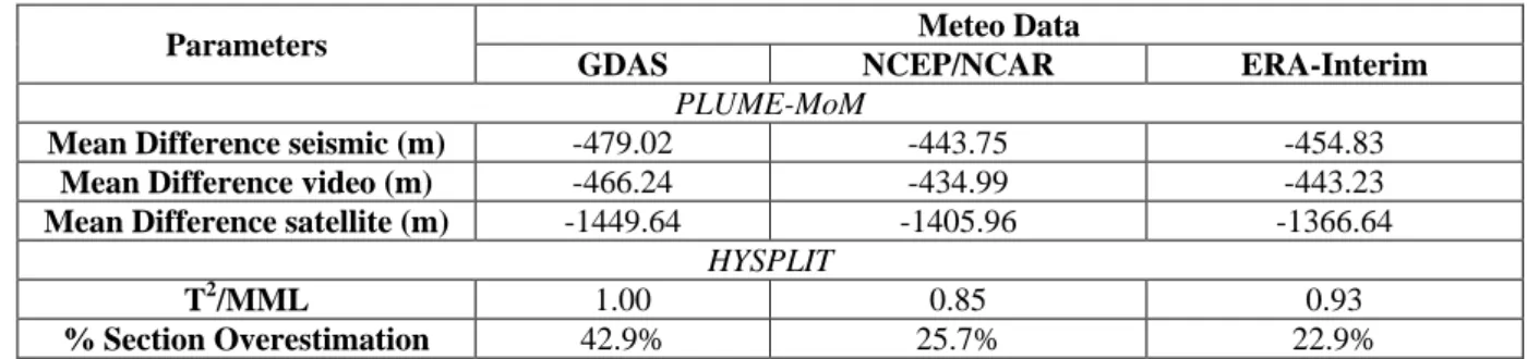
For each meteo condition and for the values of MER considered, plume heights
383
comparison (Fig. 3a) shows that PLUME-MoM results are generally lower than those
384
obtained by inverting seismic signal or from satellite/video camera images, though the model
385
data mimic the patterns of observations. The difference between observed and modeled values
386
(Table 2) is ~435-480 m for the seismic signal and video camera images while it is
~1300-387
1400 m for the satellite measurements. We note, however, a few exceptions. For the
seismic-388
derived data, exceptions are the days around the 23rd of September, where modeled plume
389
heights are systematically higher than the inferred ones. In contrast, Fig. 3a shows that there is
390
a very good correlation between modeled and observed plume heights estimated from video
391
recordings for the first phase of the eruption (August and beginning of September).
392
Ground deposits data show a difference of about 15°-20° between the directions of
393
modeled and observed main dispersal axes (Figs. 2a and 3b). Notice that the deposits
394
simulated, despite in extremely low quantities (i.e. 10-10-10-11 kg/m2) at more distal locations,
395
are spread all over the computational domain (see Figs. S1 to S3). Mass loading data show
396
that the simulations underestimate field observations at locations in the main dispersal axes
397
(Fig. 3b). Notice that the two sections along the main dispersal axes with the highest
398
underestimations (BNAS and PNC 4 sections, see Table S3 from the Supporting Information)
399
have observed mass loading values of, respectively, 18 and 15 kg/m2; for these two sections,
which are very proximal (~5 and ~7 km from the vent respectively) the model predicts very
401
low deposition (<1 kg/m2 for all the simulations). The T2/MML values (Table 2) show that the
402
differences between model and observed values are relatively low, and the model generally
403
underestimates the observed values (57% to 77%of the field sections are underestimated). An
404
area of model underestimation might be recognized close to the vent area along the main
405
dispersal axes for all the simulations (see Figure S17 from the Supporting Information). The
406
MO and MU values (and also the MO/MML and MU/MML ratios) are similar for the
407
different meteo data, and for all the cases with a higher value of MU and MU/MML (for
408
simulations done using the NCEP/NCAR and the ERA-Interim meteo data).
409
The grain size data are scarce but we note that the computed Mdφ values are almost
410
always shifted toward coarser sizes (Fig. 3c) and that the σφ values show that the sorting of
411
the computed deposit is much smaller with respect to reality (Fig. 3d). Both computed Mdφ
412
and σφ show nearly constant values for a given section but with different meteo data.
413 414
3.2 Tungurahua 2013
415
For the T13 eruption, a total of 48 mass loading measurements [unpublished and from
416
Parra et al., 2016] and 29 grain size analyses [unpublished and from Parra et al., 2016] were
417
used for the comparison (Fig. 2b).
418
The plume heights comparison (Fig. 4a) shows that all the simulations markly
419
underestimate the observations reported from both sources. The mean difference is about -2.1
420
km to -2.2 km (Table 3). The difference of deposit main dispersal axes is small since the
421
simulations done using GDAS and ERA-Interim data are almost coincident with respect to
422
field data while the NCAR simulation is only 8° shifted toward the SW (Figs. 2b and 4b).
423
The observed values of mass loading (Fig. 4b and Table S3 from the Supporting
424
Information) are all <3 kg/m2, similarly with respect to the C15 eruption for the two sections
425
along the main dispersal axes (San Pedro de Sabanag and 12 de Octubre, Table S3 from the
426
Supporting Information). Mass loading differences have a small spread highlighted by low
427
T2/MML values (Table 3). This is also shown by the absolute differences (MO and MU),
428
which are also almost identical despite the model tends to underestimate field data at most
429
sections. For the T13 eruption, the distribution of sections with overestimation and
430
underestimation does not highlight homogeneous areas of model overestimation or
431
underestimation (see Fig. S18 from the Supporting Information). In Table 3 the MO/MML
432
and MU/MML ratios have both values <1, indicating that the difference in mass loading value
433
is less important than the average deposit value of mass loading. In Fig. 4b, the mass loading
434
differences with respect to the observed data are equally positive (overestimation) or negative
435
(underestimation) in proximity of the main dispersal axes, without a clear prevalence.
436
Grain size comparison highlights that, similarly to the C15 eruption, most of the
437
computed grain sizes are shifted toward constant coarser grained values (Mdφ, see Fig. 4c)
438
with a smaller and fairly constant sorting for much of the sections (σφ, see Fig. 4d). Notice,
439
however, that some simulation sorting values are along the perfect fit line (mostly
440
NCEP/NCAR simulation) or are even larger than the observed ones (GDAS and the
ERA-441 Interim simulations). 442 443 3.3 Tungurahua 2006 444
For the T06 eruption, a total of 48 mass loading measurements [Eychenne et al., 2012]
445
and 22 grain size analyses [recalculated from Eychenne et al., 2012, see also Text S1 from the
446
Supporting Information] were used for the comparison (Fig. 2c).
Fig. 5a shows that the plume heights simulated are close to observed data, except for
448
the NCEP/NCAR model. The ERA-Interim/WRF model, in particular, provides a low mean
449
overestimation of about 400 m (Table 4). Notice that this simulation was characterized by a
450
fairly low T2 value, although higher with respect to the parent ERA-Interim simulation (Table
451
4). This difference is due to the iterative procedure described in Section 2.4, which allowed
452
finding the hourly values of MERs that minimized the differences in plume heights. Another
453
combination of MERs was instead used for the other three meteorological datasets.
454
Differences in deposit main dispersal axes are the highest of the four studied eruptions and are
455
up to about 40° toward South (see ERA-Interim meteo in Figs. 2c and 5b).
456
With respect to mass loading, the T2/MMLvalues (Table4) highlight a relatively high
457
spread of the data, which is also reflected in the MO and MU values. In this case, it could be
458
considered that most of the sections with underestimation are concentrated in proximity of the
459
main dispersal axis highlighted by field data (Fig. 5b). Notice that the NCEP/NCAR provides
460
the highest values of overestimation (MO = 62.57, MO/MML = 7.68). Moreover, the T06
461
eruption is one of the two cases, among the studied ones, where one simulation gives more
462
sections with overestimation than sections with underestimation (ERA-Interim/WRF, see
463
Table 4). Considering the spatial distribution of sections with overestimation and
464
underestimation (see Fig. S19 from the Supporting Information), then a homogeneous area of
465
model overestimation might be identified in the proximity of the vent area along the main
466
dispersal axes (see Fig. S19 from the Supporting Information). Figure 5b highlights an
467
interesting pattern for all the sections since the difference in mass loading tends to increase
468
approaching the main dispersal axis, which is particularly evident for the GDAS and the
469
NCEP/NCAR simulations.
470
The grain size data show a fairly well defined trend of Mdφ values, which are close to
471
the perfect fit line (Fig. 5c). The model sorting values are instead mostly shifted toward lower
472
values but define trends mimicking that of the perfect fit line (Fig. 5d).
473 474
3.4 Puyehue-Cordón Caulle 2011
475
For the PCC11 eruption, a total of 75 mass loading measurements and 24 grain size
476
analyses [Bonadonna et al., 2015a; Pistolesi et al., 2015; unpublished] were used for the
477
comparison (Fig. 2d). For the mass loadings, the thickness data of Pistolesi et al. [2015] were
478
multiplied by the bulk deposit density value of 560 kg/m3 reported in Bonadonna et al.
479
[2015a] for Unit I, in order to obtain kg/m2 values. Daily average plume heights a.s.l. reported
480
in Bonadonna et al. [2015b] have been converted into “above vent” values by subtracting the
481
vent elevation reported in Bonadonna et al. [2015b] (1470 m a.s.l.).
482
For this eruption, the simulations generally overestimate the plume heights observed,
483
which are lowered with the inverse procedure (see Table 5, Fig. 6a). The simulated deposit
484
main dispersal axes are all shifted toward the South by 5-10° with respect to the field data
485
(Figs. 2d and 6b).
486
For the mass loading, most of the T2/MML values are the highest among all the
487
simulations, with values up to 22.12 (ERA-Interim) (Table 5). MO and MU values are
488
respectively >100 kg/m2 and from -18 kg/m2 up to -54 kg/m2. The MO/MML and MU/MML
489
ratios indicate anyway that mean overestimation is 3 to 6 times higher than MML and that
490
mean underestimation is 0.3 to 1 times higher than MML. As for the other eruptions, the
491
percentage of sections with overestimation is lower than that with underestimation, except for
492
the simulation done with the GDAS meteo data (Table 5). From Fig. S20 from the Supporting
493
Information, the distribution of the sections with overestimation or underestimation highlights
494
a homogeneous area of model overestimation located 30-40 km from vent area along the main
495
dispersal axes. The correlation between high values of mass loading overestimation and the
position of the main dispersal axis (Figure 6b) is evident only for the simulation done with the
497
ERA-Interim meteorological data. For the other simulations instead, the sections with the
498
highest differences are uncorrelated with respect to the position of the main dispersal axis
499
given by the model. It is also important to underline that in this case also, sections with
500
highest values of observed mass loadings are not correlated with the deposit main dispersal
501
axis given by field data, a pattern that is confirmed also by the simulations (see Fig. 6b). This
502
latter feature might be correlated with the progressive anticlockwise rotation of the ash cloud,
503
a pattern already discussed by Pistolesi et al. [2015] and Bonadonna et al. [2015b]. To
504
confirm this, we have also performed a more detailed analysis using satellite images to track
505
the evolution of the ash cloud during the 04-05/06/2011: details about this method are
506
reported in Text S1 from the Supporting Information. The sequence of images derived (Figure
507
S21 from the Supporting Information) show that at the onset of the eruption the cloud drifted
508
southwestwardly (130°), but as time passed, the cloud rapidly moved towards the east,
509
reaching 105°. This compares with the main dispersal axis assessed from the field deposits
510
integrated over the whole Unit I (layers A-F) and yielding a mean direction of 117°. However,
511
the maximum mass loading of deposits have been recorded at much higher angles, lying
512
between 130-135° (Figure 6b). This actually correlates with ash emissions occurring at the
513
onset of the eruption, where the ash-rich plume might have produced rapid and en masse
514
fallouts along the main ash cloud dispersal axis centered at 130° (Figure S21 from the
515
Supporting Information). This is supported by mass loading values of the deposits, which are
516
very high on the dispersal axis (green dots in Figure S21), ranging from 481.6kg/m2 close to
517
the vent (section n° 57, Table S3 from the Supporting Information) to 160 kg/m2 at a greater
518
distance. By contrast, the mass loading of samples located away from the dispersal axis (red
519
dots in Figure S21), shows much lower values of about 5.6 kg/m2, although being close to the
520
vent. Interestingly, section n° 57 is also the one that tends to have the highest value of
521
underestimations (up to -400 kg/m2).
522
Regarding the grain size data, the Mdφ values are spread on both sides of the perfect
523
fit line (Fig. 6c). The NCEP/NCAR simulations (both direct and inverse) tend to give finer
524
grained values with respect to the observed data. The sorting data tend to define two trends of
525
constant values of σφ ~0.5 and ~2, and some model sorting values are higher than the
526
observed ones (Fig. 6d). An important remark for the modeled grain sizes of the PCC11
527
eruption is that none of them show any bimodal distribution in contrast to the observed data.
528
This is particularly evident for the above-mentioned section n° 57, which does not have
529
bimodality and which has an Mdφ shifted toward more coarser-grained values.
530 531 532
4. Discussion
533
4.1 Uncertainty in the input parameters
534
A significant amount of uncertainty in the simulations may derive from the
535
meteorological data employed. As also shown by other studies [e.g. Devenish et al., 2012;
536
Webster et al., 2012], even small errors in the wind field can lead to large errors in the ash
537
concentration, making therefore apoint-by-point comparison of modelled with observed data
538
a challenging task. The datasets we considered are among the most widely used in similar
539
numerical modellings [e.g., Webley et al., 2009; Bonasia et al., 2012; Folch, 2012; Costa et
540
al., 2016]: moreover, it has also been used the mesoscale meteorological model WRF/ARW,
541
which has been coupled with other TTDMs in similar works [e.g. FALL3D, Poret et al.,
542
2017]. From our results, it is not evident that a particular meteorological dataset provides
543
systematically the best results. For instance, the GDAS dataset provides the worst results (in
544
terms of both the T2 and the MO-MU values) for the lower magnitude C15 and T13 eruptions,
while it provides the best results for the T06 and PCC11 eruptions. The NCEP/NCAR dataset
546
shows the opposite as the results are better for the C15 and T13 eruptions with respect to T06
547
and PCC11. The employment of the WRF/ARW model (see also Text S1 from the Supporting
548
Information) did not result in a significant improvement of the results as it gave instead higher
549
T2/MML values with respect to the parent ERA-Interim meteorological file (see Table 4),
550
although for some other models the employment of the WRF/ARW model gave better results
551
[Parra et al., 2016]. Given the high computational times necessary to process original meteo
552
data, the refinement procedure using WRF/ARW was not applied to other longer eruptions.
553
The meteorological data have a considerable effect on the direction of main advection of the
554
volcanic particles, which controls the deposit main dispersal axis direction. This is
555
particularly evident for the T06 eruption, where differences with respect to the observed axis
556
are up to 40°. Two main reasons for such differences may be invoked: i) the meteorological
557
data are built in a way such that their parameters remain constant for relatively long periods (3
558
to 6 hours) and for quite large areas (0.75°x0.75° up to 2.5°x2.5°), and within such temporal
559
frames and spatial domains it is not possible to capture the variability of natural phenomena;
560
ii) 4-dimensions meteorological files (especially Reanalysis products) might be less accurate
561
over complex terrains (e.g. the Andes), for which the details of the atmospheric flow are less
562
likely captured and there are not a lot of observations available. This could be the case for the
563
T06 and T13 eruptions, where the rugged topography of the area surrounding the Tungurahua
564
volcano could have caused secondary atmospheric effects not recorded in the meteorological
565
files.
566
A common problem with eruption source parameters is the measurements of plume
567
height. For instance, for the C15 eruption Bernard et al. [2016a] used three different
568
methodologies for plume height estimates (inversion of seismic signals, video cameras
569
observations, and satellite measurements), which gave sometimes very different values (see
570
Fig. 3a). For the T06 eruption, Steffke et al. [2010] used two different methods of satellite
571
observations. Therefore, it is not surprising that differences in measurements at the same time
572
can be important. The uncertainty in plume height is also high for the T13 eruption, for which
573
two different methods (satellite measurements and visual observations) have been employed,
574
and for the PCC11 eruption as well, for which only daily mean values of plume height have
575
been reported.
576
Mass loading values for the C15, T13 and T06 eruptions have been actually measured
577
for each section (with various methods), but for the PCC11 they have been determined by
578
multiplying the deposit thickness by a mean bulk deposit density value (see Section 3.4). This
579
latter aspect is critical since density of tephra fall deposits may vary considerably owing to
580
drastic density change between different particle sizes [e.g., Bonadonna and Phillips, 2003;
581
Eychenne and Le Pennec, 2012; Pistolesi et al., 2015]. This is particularly important for the
582
PCC11 eruption that has the highest T2/MML values (see Table 5), which might also be
583
related to an uncertainty in the observed mass loading data. We also stress that the assumption
584
of a linear variation of particle density with grain size (employed in PLUME-MoM) is a
585
simplification since the density variation may be more complex [i.e sigmoidal rather than
586
linear as for the T06 eruption, Eychenne and Le Pennec, 2012]. Compared to other sources of
587
uncertainty, however, the simplification used in the simulations is expected to have a minor
588
effect on the final results.
589
Finally, it is important to remark that there are also uncertainties in estimations of the
590
initial water mass fraction in magmas. This is due primarily to the use of different methods
591
[e.g., by direct measurements, geological inference, thermodynamic calculation or
592
experimental approaches, see Clemens, 1984], among which the direct measurement from
593
melt inclusions in crystals are the most used [see for example Plank et al., 2013]. As a
594
comparison, for this study we relied on estimates made both using direct measurements from
melt inclusions and experimental approaches [Martel et al., 2018] or considering only
596
experimental approaches [Andújar et al., 2017]: results gave H2O wt. % ranging between 4-6 597
wt. % and 6-8 wt. .% for andesites and rhyolites respectively. As the water mass fraction has a
598
strong influence on the plume height simulated with PLUME-MoM [see section 2.2.1 and
599
also de'Michieli Vitturi et al., 2016], its careful estimation is therefore of primary importance.
600 601
4.2 Uncertainty in the numerical modelling
602
When MER values obtained from total deposit measurements are used as input
603
parameters, PLUME-MoM underestimates the plume height measurements for three out of
604
four eruptions tested, and there may be two main reasons for that. First, as already discussed
605
in the previous section, the measurements are in some specific cases uncertain. Second, the
606
mass eruption rate, assumed to be equal to the total mass of deposit divided with the eruption
607
duration, may be underestimated in some cases (e.g. the T06 eruption) since deposits of
608
pyroclastic density currents are neglected, hence giving lower plume heights. We note,
609
however, that the mean underestimations (and mean overestimations as well) of the model for
610
each eruption are lower with respect to the uncertainty in observed data among different
611
methods, and that in some cases (e.g. the T06 eruption) the refinement of the meteorological
612
data using the WRF/ARW model can sensibly reduce the difference in plume height with
613
respect to observed data.
614
The PLUME-MoM/HYSPLIT model tends generally to have more points
615
underestimating the mass loading data (see Tables 2 to 5). However, if the absolute mean
616
differences (MO and MU) and their ratios with mean values of mass loading (MO/MML and
617
MU/MML) are considered, then model overestimation is systematically higher with respect to
618
underestimation. For example, for the PCC11 eruption and for the simulation done using the
619
ERA-Interim data, MO is almost 10 times higher than MU (Table 5). The high values of MO
620
or MU and of their ratios with MML tend also to be higher for higher magnitude eruptions
621
(e.g. T06 and PCC11): in this regard the inverse procedure reduces considerably the
622
discrepancy between modeled and observed data as indicated for instance by the T2/MML
623
value for the PCC11 eruption.
624
The problem of model uncertainty is further illustrated by the difference in mass
625
loading with respect to the orientation of the stratigraphic section (Figs. 3b, 4b, 5b and 6b).
626
There are two opposite situations since the deposit main dispersal axis coincides either with
627
the lowest values of Δ mass loading (highest underestimation, e.g. C15 eruption, Fig. 3b) or
628
with the highest values of Δ mass loading (highest overestimation, T06 eruption, Fig. 7b, and
629
to a lesser extent T13 and PCC11 eruptions). This may be explained considering the advective
630
and diffusive parts of the transport equation used [Folch, 2012]. While the mass seems to be
631
correctly advected in the simulations (although with some deviation with respect to observed
632
data), the equations of HYSPLIT related to turbulent diffusion do not appear to work
633
efficiently, underestimating the horizontal diffusion and concentrating the mass close to the
634
main dispersal axis of advection. A similar issue has been also encountered by Hurst and
635
Davis [2017]. This may explain the above-mentioned mass loading underestimation or
636
overestimation, which are possibly increased by the fact that the HYSPLIT model does not
637
account for complex collective settling mechanisms of volcanic ash caused by aggregation,
638
gravitational instabilities, diffusive convection, particle-particle interactions and wake-capture
639
effects [Del Bello et al., 2017; Gouhier et al., 2019]. However, the problem of the effect of
640
diffusion on volcanic plumes dispersal and therefore on particle sedimentation is complex
641
[see for example Devenish et al., 2012]: a more rigorous study is therefore needed for
642
HYSPLIT to investigate the influence of different available diffusion equations on final
643
results.
The failure to take into account such mechanisms implies that the simulated
finest-645
grained particles are transported much further that in reality. For instance, the C15 eruption
646
has a particularly fine-grained TGSD [due also to its hydrovolcanic nature, Bernard et al.,
647
2016a] (see Table S2 from the Supporting Information) so that the mass is transported all over
648
the computational domain (see Figs. S1 to S3 from the Supporting Information). The case of
649
the PCC11 eruption is similar since the TGSD is up to 12φ, and an estimated amount of ~5%
650
of the erupted mass is transported out of the computational domain. While for this eruption
651
the finest fraction of the volcanic clouds circumvented the Southern hemisphere and passed
652
over the South of Australia [Collini et al., 2013], it is possible that part of the fine ash did not
653
deposit (see also the issue of grain size analyses in the following paragraph). In this context,
654
the transport of material could have been at its maximum along the main dispersal axes, and
655
therefore the degree of underestimation of mass loading at proximal-medial sites along
656
dispersal axes is maximized as well.
657
Regarding the simulated grain size data, the Mdφ values are systematically
coarser-658
grained for the C15 and T13 low magnitude eruptions while they are either coarser-grained or
659
finer-grained for the PCC11 eruption. The shifting toward coarser-grained Mdφ values can be
660
explained by the fact that HYSPLIT neglects the above-mentioned collective settling
661
mechanisms of volcanic ash. For the eruptions where the amount of fine ash is higher (the
662
C15, T13 eruptions and partially the PCC11 one), the fine ash is transported distally, hence
663
causing coarser grain sizes in proximal to medial sections. Moreover, the model is not capable
664
of reproducing the bimodality of grain size distribution observed, as for instance in the PCC11
665
eruption. The σφ comparisons show that, instead, for most cases the modeled data tend to
666
have a lower sorting value with respect to the observed ones. These results show that the
667
employment of grain size data for model validation is less reliable with respect to mass
668
loading data.
669
Four important issues should be considered to improve the coupled
PLUME-670
MoM/HYSPLIT model in the context of tephra fallout hazard assessments and probabilistic
671
hazard maps production. First, the meteorological dataset must be considered carefully since
672
it controls strongly the plume height. Second, the amount of fine ash and the duration of the
673
eruption seem to be more critical than the magnitude of the eruption for mass loading
674
calculations, since the simulations of higher magnitude eruptions of short duration with lower
675
wt% of fine particles (i.e. T06 eruption) are more accurate than simulations of lower
676
magnitude eruptions with longer durations and a higher amount of fines (i.e. the C15 and
677
T13). If the magnitude, the amount of fine particles and the duration of the eruption are high
678
(i.e. the PCC11 eruption), then the model tends to overestimate the natural data. Third, for the
679
above-mentioned reasons, we recommend to employ PLUME-MoM/HYSPLIT in its present
680
configuration for the production of hazard maps related to higher magnitude eruptions (i.e.
681
sub-Plinian or Plinian). This is supported by our simulations of such eruptions (i.e. T06 and
682
PCC11), for which overestimation is much higher (in terms of mean absolute values) with
683
respect to underestimation. This latter point is important in a context of hazard assessment
684
since underestimation may be considered as less acceptable than overestimation. Moreover, it
685
is also important to remind that: a) specifically for our test eruptions, the lower magnitude
686
ones tend to have longer durations and are more difficult to model due to the very high
687
variability of both the eruptions parameters and atmospheric conditions, which are less likely
688
to be captured; b) the T06 and PCC11 eruptions are those for which modeled and observed
689
plume heights are more similar. Fourth, the MO/MML and MU/MML ratios may be used to
690
account for model uncertainty and to serve as a basis for calculating coefficients that allow the
691
creation of probabilistic maps (from the point of view of mass loading) that quantify the
692
model mean overestimation and underestimation. For this purpose, statistical techniques
693
might be employed to correct the model by estimating its deviance from the observed data.