Random sampling and machine learning to understand good decompositions

(1)

HAL Id: hal-02319521

https://hal.inria.fr/hal-02319521

Submitted on 18 Oct 2019

HAL is a multi-disciplinary open access

archive for the deposit and dissemination of

sci-entific research documents, whether they are

pub-lished or not. The documents may come from

teaching and research institutions in France or

abroad, or from public or private research centers.

L’archive ouverte pluridisciplinaire HAL, est

destinée au dépôt et à la diffusion de documents

scientifiques de niveau recherche, publiés ou non,

émanant des établissements d’enseignement et de

recherche français ou étrangers, des laboratoires

publics ou privés.

Random sampling and machine learning to understand

good decompositions

Saverio Basso, Alberto Ceselli, Andrea G. B. Tettamanzi

To cite this version:

Saverio Basso, Alberto Ceselli, Andrea G. B. Tettamanzi. Random sampling and machine learning

to understand good decompositions. Annals of Operations Research, Springer Verlag, 2020, 284 (2),

pp.501-526. �10.1007/s10479-018-3067-9�. �hal-02319521�

(2)

Noname manuscript No.

(will be inserted by the editor)

Random Sampling and Machine Learning to Understand

Good Decompositions

S. Basso

· A. Ceselli

? ??

· A. Tettamanzi

the date of receipt and acceptance should be inserted later

Abstract

Motivated by its implications in the development of general purpose

solvers for decomposable Mixed Integer Programs (MIP), we address a

funda-mental research question, that is to assess if good decomposition patterns can be

consistently found by looking only at static properties of MIP input instances, or

not. We adopt a data driven approach, devising a random sampling algorithm,

considering a set of generic MIP base instances, and generating a large, balanced

and well diversified set of decomposition patterns, that we analyze with machine

learning tools. The use of both supervised and unsupervised techniques highlights

interesting structures of random decompositions, as well as suggesting (under

cer-tain conditions) a positive answer to the initial question, triggering at the same

time perspectives for future research.

1 Introduction

General purpose Mixed Integer Programming (MIP) solvers have been developed

for decades from both theoretical, algorithmic and software engineering points

of view. There is indeed a huge interest in making such tools more and more

effective, the primary one being their ease of integration in real world decision

support systems [4, 5, 6].

?

_{The work has been partially funded by Regione Lombardia – Fondazione Cariplo, grant}

n. 2015-0717, project REDNEAT, and partially undertook when the second author was visiting

INRIA Sophia Antipolis - I3S CNRS Universit´

e Cˆ

ote d’Azur.

??

_{Corresponding: A. Ceselli, Universit`}

_{a degli Studi di Milano, Dipartimento di Informatica,}

Via Bramante 65 - 26013 Crema (CR) - Italy - Tel. +39 0373 898052)

S. Basso

Universit`

a degli Studi di Milano, Dipartimento di Informatica, svr.basso@gmail.com

A. Ceselli

Universit`

a degli Studi di Milano, Dipartimento di Informatica, alberto.ceselli@unimi.it

A. Tettamanzi

(3)

Fig. 1 Structure of a MIP with diagonal blocks (black) and border (grey).

All state-of-the-art solvers currently rely on complex methods mounted on

branch-and-cut frameworks, where Linear Programming (LP) relaxations are used

to produce initial dual bounds, that are subsequently strengthened by cutting

planes [2]. On the one hand such a paradigm offers efficiency and stability, coming

from a deep computational understanding built over the years; on the other hand,

such a structure yields to drawbacks that show to be very hard to overcome by

simply plugging in additional techniques.

A key one is related to the structure of models: while on the majority of the

cases generic cutting procedures are very effective, on a few classes of combinatorial

optimization problems the initial LP dual bounds are too poor to drive the full

method. A second weakness is related to the structure of algorithms, preventing

them to scale effectively as the amount of available computing resource increases,

for instance thanks to multi-core or distributed computing capabilities.

To overcome these drawbacks, at least when well-structured combinatorial

op-timization problems need to be optimized, researchers have started to

investi-gate alternative paradigms. One of them is Dantzig-Wolfe decomposition applied

to integer programs (DWD): on applications like vehicle routing, crew

schedul-ing, cutting stock, facility location, generalized assignment, and many others [13],

DWD-based techniques proved to be far superior to branch-and-cut. In fact,

mod-els for these applications exist, having as common structure a constraint matrix

in a so-called bordered block-diagonal form (see Figure 1). DWD is able to

disag-gregate these problems in a master entity, involving only constraints and variables

in the border, and one or more subproblems, one for each diagonal block. DWD

can then be paired with column generation techniques [1] to obtain dual bounds

that are potentially much tighter than the LP relaxation of the original model

in reasonable computing time. Furthermore, these column generation techniques

prove to scale very well as the amount of computing resources increases [22].

DWD has however, one fundamental issue preventing it to be applied as

gener-ically as cutting planes: decomposition patterns must be provided by the modeler,

and such a task requires deep mathematical programming skills. That is why,

although many positive results have been obtained by problem-tailored DWD

ap-proaches, very few attempts have been made in the literature to tackle MIPs with

generic

DWD methods.

All of them aim at analyzing a MIP, understanding whether a suitable

struc-ture can be detected, and automatically performing DWD and column generation.

A few research threads can be surveyed in the literature. The first one considers

to explicitly enrich the input, asking the user both a MIP instance (as in current

(4)

branch-and-cut based general purpose solvers), and a decomposition pattern

de-scribing the block structure to be exploited. DWD is then applied automatically.

Approaches along this line include [14], [16] and [15]. In [9] a full generic column

generation framework is introduced, which is currently engineered and released

with the SCIP framework [10]. Since finding suitable decomposition patterns

re-quires very specific technical expertise, a second research thread is to ask only a

MIP instance as input, and to detect if in that instance specific

previously known

structures occur, which are known to be suitable for DWD. Successful

contribu-tions along this axis are indeed embedded in [9]. A third, more ambitious, thread

is to assume that

previously unknown

decomposable structure may be found (or

even

enforced

) in a generic MIP instance provided as input, that can be made

evi-dent through a suitable algorithmic search for good decomposition patterns. Very

recently, the authors of [12] propose to preprocess the input MIP with machine

learning tools, to detect first of all if it is amenable for a successful decomposition

approach or not. In [11] and [3] fully automatic frameworks are proposed,

obtain-ing better results than CPLEX [4] on a noticeable set of MIP instances. A common

issue of these approaches is to find suitable

optimization metrics

, exploiting MIP

instance details to score decomposition candidates.

Indeed a fundamental research question remains open, that is to assess if good

decomposition patterns can consistently be found at all by looking only at static

properties of the instance, or not, and possibly to understand which properties are

worth considering.

In this paper we try to step towards the clarification of this issue with an

agnos-tic approach. That is, we consider generic MIP instances and we generate a large,

balanced and well diversified set of decomposition patterns. Then we analyze them

with statistical and machine learning tools, with the main aim of understanding

if good ones can be distinguished from others by automatic methods looking only

at the static properties of the corresponding matrices.

We formally employ both supervised and unsupervised learning tools [19]

al-though, whenever possible, we present our methods with an operations research

language and perspective. Indeed using Machine Learning for Integer

Program-ming [24] or vice versa [23], and in general integrating both fields [25], is a recent

and extremely promising trend.

The paper is organized as follows. First we face the key issue of producing a

sig-nificant dataset, proposing a randomized sampling algorithm (Section 2); we then

perform a preliminary assessment on the properties of such a dataset (Section 3).

Second, we check if simple correlation patterns arise, linking single properties of

the MIP instance to the computational behavior of decompositions (Section 4).

Since no particular pattern is found by this check, we perform more advanced

analyses for finding out if

combinations of MIP instance properties

can be used to

effectively predict how good a decomposition is (Section 5). We finally estimate

which is the impact of exploiting previous knowledge of good and bad

decomposi-tions, both on the same and on different MIP instances, in correctly understanding

new decompositions (Section 6). Our research leads to some perspectives, which

are collected in a final discussion (Section 7).

(5)

– Fix the initial set of blocks to be empty.

– Consider a special border block, which is initially empty.

– At each iteration, assume that a set of blocks has already been created; a new constraint

is chosen at random, with a probability directly proportional to its sparsity, defined as

the number of zeros in the constraint matrix

– if the constraint covers no variable that is covered by other constraints belonging

to existing blocks, then a new block is created, and the constraint is assigned to

that block

– if the constraint covers any variable that is covered by other constraints belonging

to more than one existing block, then the constraint is put in the border

– if the constraint covers variables that are covered by constraints in a single

existing block, and possibly additional variables that are still uncovered, then the

constraint is added to that block.

Fig. 2 Randomized algorithm for sampling decompositions.

2 Dataset generation

Our first target was the creation of a significant and well diversified dataset, as

a key requirement for our investigation was to have both

good and bad

decompo-sition to compare. This task turned out to be difficult: on one hand, drawing a

random decomposition for an arbitrary MIP is very likely to yield unpromising

results; on the other hand, focusing on specific good decomposition patterns for

known decomposable MIPs would not allow to produce both diversified positive

and negative examples. Indeed, many of our initial attempts to produce diverse

decompositions failed in either sense, as it was very hard to produce a sufficiently

large and spread sampling, and make at the same time block diagonal structures

appear in the coefficients matrix; in turn, no block structure basically means a

predictably useless decomposition approach.

We finally found the following approach to produce meaningful results. We

considered a set of

generic base MIP instances

(base instances in the remainder),

selecting them from

unstructured

problems in MIPLIB 2003 [7] and MIPLIB 2010

[8] that, according to [3], might potentially be suitable for a decomposition

ap-proach. The list of our base instances is reported in Section A.1 of the appendix.

These are all stated as minimization problems. For each base instance we generated

1000 random decompositions with the randomized sampling algorithm reported in

Figure 2. It builds blocks of constraints, that in turn induce blocks of

correspond-ing

covered

variables, that is variables having nonzero coefficients in the constraints

of the block.

The randomized algorithm produces decompositions with a random number

of blocks; we fixed a minimum blocks threshold: when a decomposition was

pro-duced, containing fewer blocks than the threshold we simply repeated the

gener-ation process, until that criterion was met. Such a threshold was fixed to 3 in our

experiments.

Then, each decomposition was analyzed, and a set of

features

was extracted

by measuring standard properties of both the constraint matrix, the constraints

right hand sides and the objective function coefficients of variables in each block.

A full list of the features is reported in Section A.2 of the appendix. These include

also the quality measures that were employed in the decomposition optimization

algorithms of [3]. We have also introduced a coefficient to estimate how similar

is each block to a totally unimodular matrix: intuitively total unimodular blocks

mean decomposition subproblems possessing the integrality property, and

(6)

there-For each block independently

– if any variable of the block contains more than two non-zero entries, return 0.0

– if any entry in the block is different from 0, 1 or −1, return 0.0

– initialize a left and right partition to be empty sets

– initialize a counter k = 0

– iteratively, consider each variable of the block in the order in which they appear in the

base instance:

– if the number of its non-zeros entries in the block is either zero or one, increase k

and iterate

– if the variable has two different entries in the block, corresponding to constraints

assigned to different partitions, increase k and iterate

– if the variable has two equal entries in the block, corresponding to constraints

assigned to the same partition, increase k and iterate

– if the variable has two different (resp. equal) entries in the block, one of which in

a constraint assigned to a certain partition, and the other in a constraint assigned

to no partition yet, assign the second constraint to the opposite (resp. the same)

partition, increase k and iterate

– if the variable has two different (resp. equal) entries in the block, none of which

in a constraint assigned to a partition, choose a random partition, assign the first

constraint to it, and the second constraint to the other (resp. the same) partition,

increase k and iterate

– otherwise simply iterate without increasing k

– return k divided by the total number of variables appearing in the block.

Fig. 3 Computation of a Total Unimodularity coefficient.

fore yielding no bound improvement in a DWD-like decomposition process. Sets

of conditions being sufficient for proving total unimodularity require, for instance,

to find a suitable bi-partition of the set of rows [26]: in an effort to obtain a

nu-merical feature, we approximated such a check by means of a randomized greedy

algorithm, whose pseudo-code is reported in Figure 3.

The randomized greedy algorithm was iterated ten times, and the highest value

was retained as final coefficient. The coefficient represents the fraction of variables

that have been considered before stopping in a failure status. That is, in the

ex-treme cases, 1

.

0 means that the corresponding matrix has been proved to be totally

unimodular (that is undesirable for the decomposition process), while 0

.

0 means

it has been proved not to be totally unimodular.

Afterwards, we ran a simulation on each decomposition, experimentally solving

the continuous relaxation of the corresponding extended formulation, that is

com-puting the corresponding dual bound at the root node of a branching tree. Such a

simulation was carried our by means of the generic column generation procedure of

GCG [9] from the SCIP framework [10], excluding all preprocessing, cut generation

and problem reduction procedures, and activating IBM ILOG CPLEX 12.6.3 [4] to

solve LPs. Bash and Python scripts were used to manage the whole process. The

result of each simulation was a dual bound value and a corresponding computing

time for each decomposition. No time limit was given to the simulations, but a

very limited number of runs did not terminate after weeks of computing. Those

were marked as “timeout”; obtaining a valid dual bound was always possible, even

on timeout instances.

After preliminary experiments we decided to remap time values in a base 10

logarithm scale. Both time and bound were then transformed into scores in the

range [0

,

1] through a feature scaling normalization, using as limits the maximum

and minimum values on the decompositions of the same base instance. That is, we

assigned higher scores to high bounds and low computing times: decompositions

(7)

that reached the time limit received score 0 in computing time whereas those that

had maximum (resp. minimum) values in bound (resp. time) received score 1.

After all decompositions related to a certain base instance were processed, each of

them was marked as positive or negative according to the following relaxed Pareto

optimality definition.

Let

A

and

B

be two decompositions for the same base instance, let

b

A

and

b

B

be the dual bound scores they yield, and let

t

A

and

t

B

be the computing time

scores required to achieve them. We define decomposition

A

to be

dominated

by

decomposition

B

if and only if

b

A

· (1 +

β

)

≤ b

B

and

t

A

· (1 +

τ

)

≤ t

B

, where

β

and

τ

are two tolerance parameters that we use to control how many decompositions

can be considered comparably good.

In particular, for the time tolerance

τ

we evaluated 10 logarithmic spaced

val-ues from 1% to 100%, while for the bound we evaluated 10 linearly spaced valval-ues

from 0.1% to 10%. After fixing

β

and

τ

, each decomposition that was dominated by

no other was marked as

positive

, all the remaining ones as

negative

. These boolean

marks were added to the dataset as class labels. Bounds and computing time were

recorded, but excluded from the set of features, as they are not statically

observ-able, and therefore unsuitable as input in a hypothetical decomposition generation

process.

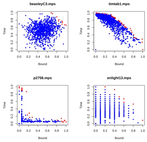
In Figure 4 (resp. 5) we report the average number of positive decompositions

for every value of

τ

(resp.

β

) over every possible value of

β

(resp.

τ

). Variations

on

τ

have a sharp effect on the number of Pareto optimal decompositions whereas

variations on

β

have a more limited impact.

We performed experiments on several tolerance configurations, finding the

fol-lowing two to be more representative of the general behavior of our methods:

–

Tolerance L (Low): with 13% tolerance

τ

on time and 0.77% tolerance

β

on

bound,

–

Tolerance H (High): with 21% tolerance

τ

on time and 10.00% tolerance

β

on

bound.

For the analysis performed in the following sections we therefore report results

considering both settings.

3 A preliminary analysis of the dataset

As reported, the initial dataset was composed by 39 base instances, and 1000

decompositions for each of them. Three base instances were then excluded, as

0 0,2

0,4

0,6

0,8

1 1,2

0 2000

4000

6000

8000

10000

12000

14000

16000

18000

20000

Tolerance

Pare

to

Fig. 4 Average number of positive

decom-positions (time)

0 0,02

0,04

0,06

0,08

0,1

0,12

0 1000

2000

3000

4000

5000

6000

7000

8000

9000

Tolerance

Pare

to

Fig. 5 Average number of positive

decom-positions (bound)

(8)

●

● ● ●

●

● ● ●

●

● ●●

●

● ●●

●

0.0

0.2

0.4

0.6

0.8

1.0

0.0

0.2

0.4

0.6

0.8

1.0 beasleyC3.mps

Bound

Time

●

● ●●

●

● ●●

●

● ● ●

●

● ●●

●

● ● ●

●

0.0

0.2

0.4

0.6

0.8

1.0

0.0

0.2

0.4

0.6

0.8

1.0 timtab1.mps

Bound

Time

●

● ●●

●

0.0

0.2

0.4

0.6

0.8

1.0

0.0

0.2

0.4

0.6

0.8

1.0 p2756.mps

Bound

Time

●

0.0

0.2

0.4

0.6

0.8

1.0

0.0

0.2

0.4

0.6

0.8

1.0 enlight13.mps

Bound

Time

●

● Fig. 6 Bound and time scores for each decomposition on different base instances. Red (resp.

blue) points indicate positive (resp. negative) decompositions.

their decompositions went systematically timeout. Duplicate records (about 4%)

were discarded as well. The relevant features of the dataset were normalized with

a simple criterion: measures on the number of variables of each decomposition

were divided by the number of variables of the corresponding base instance; the

same was done for the constraints. The dataset obtained after these operations

consisted of 34565 records and 117 features. About 2% and 14% of decompositions

were classified as positive respectively with tolerance L and tolerance H.

As far as the dimensionality of the dataset is concerned, we found through a

Principal Component Analysis (PCA) 22 components to be significant according to

the eigenvalues criterion [20]. However, all these components had a correlation near

zero to both time and bound scores. Indeed, we performed many of the subsequent

experiments also by considering this set of 22 components instead of the full set

of original features. No quality increase was obtained, and at the same time we

encountered no particular computational bottleneck. Therefore we present only

results on the dataset using the full set of features.