Modeling and Verifying Uncertainty-Aware Timing Behaviors using Parametric Logical Time Constraint

HAL Id: hal-02429533

https://hal.archives-ouvertes.fr/hal-02429533

Submitted on 6 Jan 2020

HAL is a multi-disciplinary open access

archive for the deposit and dissemination of

sci-entific research documents, whether they are

pub-lished or not. The documents may come from

teaching and research institutions in France or

abroad, or from public or private research centers.

L’archive ouverte pluridisciplinaire HAL, est

destinée au dépôt et à la diffusion de documents

scientifiques de niveau recherche, publiés ou non,

émanant des établissements d’enseignement et de

recherche français ou étrangers, des laboratoires

publics ou privés.

Modeling and Verifying Uncertainty-Aware Timing

Behaviors using Parametric Logical Time Constraint

Fei Gao, Frédéric Mallet, Min Zhang, Mingsong Chen

To cite this version:

Fei Gao, Frédéric Mallet, Min Zhang, Mingsong Chen. Modeling and Verifying Uncertainty-Aware

Timing Behaviors using Parametric Logical Time Constraint. DATE 2020 - Design, Automation and

Test in Europe Conference, Mar 2020, Grenoble, France. �hal-02429533�

Modeling and Verifying Uncertainty-Aware Timing

Behaviors using Parametric Logical Time Constraint

Fei Gao

, Frederic Mallet

, Min Zhang

, Mingsong Chen

∗_{Shanghai Key Laboratory of Trustworthy Computing, East China Normal University, Shanghai, 200062, China} † _{Université Cote d’Azur, CNRS, Inria, I3S, Nice, France}

‡ _{Shanghai Institute of Intelligent Science and Technology, Tongji University, Shanghai, 200062, China}

Abstract—The Clock Constraint Specification Language (CCSL) is a logical time based modeling language to formalize timing behaviors of real-time and embedded systems. However, it cannot capture timing behaviors that contain uncertainties, e.g., uncertainty in execution time and period. This limits the application of the language to real-world systems, as uncertainty often exists in practice due to both internal and external factors. To capture uncertainties in timing behaviors, in this paper we extend CCSL by introducing parameters into constraints. We then propose an approach to transform parametric CCSL constraints into SMT formulas for efficient verification. We apply our approach to an industrial case which is proposed as the FMTV (Formal Methods for Timing Verification) Challenge in 2015, which shows that timing behaviors with uncertainties can be effectively modeled and verified using the parametric CCSL. Index Terms—Uncertainty, timing behavior, logical time, para-metric CCSL, SMT

I. Introduction

Model-based design has achieved industrial success in de-veloping safety-critical real-time and embedded systems. It introduces formal and abstract approaches to capture unam-biguously the requirement and design of systems and guar-antees correct refinement down to implementation. MARTE(a UML Profile for Modeling and Analysis of Real-Time and Embedded systems) [1] is such a approach for the specifi-cation, design, and verification/validation stages of real-time and embedded systems, and attracting considerable interest from both academia and industry. The Clock Constraint Spec-ification Language (CCSL) [2] is a companion language of MARTE, dedicated to model timing behaviors of systems using logical time constraints. Several sophisticated tools have been developed for formal verification of the language [3], [4]. Although logical time and multiform time bases in CCSL offer some flexibility to unify functional requirements and performance constraints, there is a limitation making the language hardly applicable to real-world systems. That is, CCSL cannot capture the timing behaviors that contain un-certainties despite the fact that uncertainty usually exists in realistic real-time and embedded systems [5]. In particular, uncertainty in time is common due to variable execution times caused by complex off-the-shelf processors (COTS) [6] and uncertain response times caused by complex interactions of an unpredictable environment. A task may also be affected by various uncertain factors, such as wind speed, temperature, light intensity, leading to different execution times.

To mitigate the situation, in this work we explore how to capture uncertainties in timing behaviors in a flexible way

using logical time. In particular, we consider four common timing uncertainties in execution time, period, jitter and drift. Jitter and drift are the deviations from true periodicity of a presumably periodic signal. The deviations will be corrected before the next execution in the jitter, but accumulate for all next executions in the drift. To capture the four uncertainties, we extend the CCSL by introducing parameters into con-straints. The parameters are integer variables in some intervals. A constraint with parameters represents a timing behavior with some uncertainty. We call the extension Parametric CCSL.

We then propose an approach to encode parametric CCSL into SMT formulas for efficient verification. Thanks to state-of-the-art SMT solvers such as Z3 [7], encoded SMT formulas can be efficiently solved. A recent work has shown that SMT is efficient for various verifications of CCSL, e.g., scheduling analysis and LTL model checking[4]. By encoding parametric CCSL constraints into SMT formulas, we show that SMT is also applicable to the verification of parametric CCSL.

To demonstrate the effectiveness of the proposed approach in modeling and verifying uncertainty-aware timing behavior systems, we conduct two case studies, including an industrial example which was proposed by Thales in 2015 as the For-mal Methods for Timing Verification (FMTV) challenge [8], which is an aerial video tracking system used in intelligence, surveillance, reconnaissance, tactical and security applications, characterized by strict and less strict constraints on timing.

Our work compares to the most common attempts to use generic formalisms like parametric time automata [9] or para-metric process algebras [10] to model timing behaviors with uncertainty, but advocates for the use of logical clocks as a complement to real-valued clocks. We take full advantage of CCSL in modeling, such as the flexibility provided by logical time, multi-form time bases, unified expressing of both functional requirements and extra performance constraints.

In summary, the contributions of this paper include: 1) Extension of CCSL with parameters to support modeling

uncertainty-aware timing behaviors and encoding of para-metric CCSL constraints into SMT formulas.

2) Application of the approach to the FMTV 2015 challenge in modeling and verifying an aerial video tracking system. The rest of this paper is organized as follows. Section II introduces four typical timing uncertainties considered in this work. Section III presents CCSL, its parametric extension and the encoding approach to SMT. Section IV presents two case studies. Section V finally concludes the work.

II. Uncertainties in Timing Behaviors

In this work, we only focus on four kinds of uncertainties that commonly occur in timing behaviors, i.e., uncertainties in execution time, period, drift and jitter.

1) Uncertainty in execution time: The execution time of a timing behavior is usually uncertain due to various internal and external factors such as the execution speed of a CPU is affected by the temperature. Therefore, the execution time of a timing behavior is usually represented by two arguments, which are the best and worst execution times. We use l and u to denote the two arguments, respectively. A value in the interval [l, u] is considered a valid execution of the behavior.

2) Uncertainty of period: Like execution time, the period of periodic timing behaviors may be uncertain. For instance, in the initial design of an embedded system, the period of a task may not be fixed. Designers may assume a lower bound and an upper bound for the period. It is desired to formalize such uncertainty in the design and to determine a feasible value for the period of the task during verification of the design.

For a timing behavior with a fixed period, there may be un-certainties due to the physical nature of devices. For instance, designers always use voltage transitions to capture timing information, and convert the analog signal into the digital domain for digital signal processing (DSP) [11]. However, in practice there is always a small variation of the timing signal’s rising and falling edges, which makes the timing information not as accurate as we expect in the ideal case. The arrival time of a periodic task may drift away, compared with the ideal arrival time. There are two basic kinds of drifting uncertainties called drift and jitter, explained below.

3) Uncertainty of drift: In the case of drift, the drifting of a periodic behavior accumulates for all future execution. More precisely, a task with a period p and drift d can execute every xi time units for the ith execution, where xi∈ [p − d, p+ d].

4) Uncertainty of jitter: In the case of jitter, the drifting of a periodic behavior must be corrected in the next execution. Assume that there is a task S with period p and jitter d. Task S can have its ithexecution no more than d time units before or after the time of S ’s ideal ithexecution when no jitter occurs.

Fig. 1: The example of periodicity, jitter and drift Figure 1 depicts the differences of a fixed period, jitter and drift. As for the task with jitter, it can only start before or after d time units around the dashed line, which shows the starting point of each period when the task is strictly periodic.

III. CCSL and its Parametric Extension

In this section, we first briefly introduce CCSL, and then extend to parametric one to formalize the four kinds of timing

TABLE I: The syntax and semantics of core CCSL

Constraint:φ Semantics: {δ | δ |= φ} Name a[d] ≺ b ∀n ∈ N+.(Hδ(b, n) − Hδ(a, n)= d) ⇒ (b < δ(n)) Precedence a4 b ∀n ∈ N+.Hδ(a, n) ≥ Hδ(b, n) Causality a ⊆ b ∀n ∈ N+.(a ∈ δ(n)) ⇒ (b ∈ δ(n)) Subclock a# b ∀n ∈ N+.(a < δ(n)) ∨ (b < δ(n)) Exclusion a, b + c ∀n ∈ N+.(a ∈ δ(n)) ⇔ (b ∈ δ(n) ∨ c ∈ δ(n)) Union a, b ∗ c ∀n ∈ N+.(a ∈ δ(n)) ⇔ (b ∈ δ(n)) ∧ (c ∈ δ(n)) Intersection a, b ∧ c ∀n ∈ N+.Hδ(a, n)= max(Hδ(b, n), Hδ(c, n)) Infimum a, b ∨ c ∀n ∈ N+.Hδ(a, n)= min(Hδ(b, n), Hδ(c, n)) Supremum a, b $ d ∀n ∈ N+.Hδ(a, n)= max(Hδ(b, n) − d, 0) Delay a, b $ d on c∀n ∈ N_{(b ∈ δ(m) ∧ H}+.(a ∈ δ(n)) ⇔ (c ∈ δ(n) ∧ ∃m ∈ N0 +·

δ(c, n, m)= d)) DelayFor

a, b ∝ p ∀n ∈ N_{mod p}+.(a ∈ δ(n)) ⇔ (b ∈ δ(n) ∧ (H_{= 0)} δ(b, n)+ 1)Periodicity

uncertainties. We also propose an encoding approach from parametric CCSL constraints into SMT formulas.

A. The Core CCSL

In CCSL, a timing behavior (e.g., a task sending/receiving a data, writing in a memory) is formalized by a set of logical clocks. A logic clock has two actions, i.e., tick and idle. Tick means the corresponding behavior is occurring, and idle means not. Logical clocks are controlled by a scheduler to tick or idle. Definition 1 (Logical clock): A logical clock c is an infinite sequence (ci)i∈N+, where each ci can be tick or idle.

As Lamport has pointed out, any countable set can be used to measure the passing of time [12]. Natural numbers are used in CCSL. Similarly to synchronous languages [13], logical clocks are comparable using a synchronous schedule.

Definition 2 (Schedule): Given a set C of clocks, a schedule on C is a function δ : N+→ 2|C| _{and ∀i ∈ N}+_{.δ(i) , ∅.}

Intuitively, δ(i) ⊆ C is the set of clocks that tick at step i, and iis called the step or the instant in synchronous terminology. Furthermore, empty steps will be excluded from the schedule because they do not affect logical relations on clocks.

To measure time one needs to count the number of ticks of a given clock taken as reference. Contrary to physical models that use a single global reference, logical clocks use histories to define the relations of clocks. Each clock has a memory to record the number of ticks.

Definition 3 (History): Given a schedule δ : N+→ 2|C| _{on a}

set C of clocks, a history of δ is a function Hδ: C × N+→ N

such that for each clock c ∈ C and natural number i ∈ N+: Hδ(c, i)=          0 i f i= 1 Hδ(c, i − 1) i f i> 1 ∧ c < δ(i − 1) Hδ(c, i − 1)+ 1 i f i > 1 ∧ c ∈ δ(i − 1)

For simplicity, we also write H0_δ(c, i, j) for Hδ(c, j) − Hδ(c, i) to denote the number of ticks of clock c from step i to j. Furthermore, Hδ(c, i) and H_δ0(c, i, j) may be written as H(c, i) and H0(c, i, j) for the sake of simplicity in the context.

There are two classes of CCSL constraints. One is the class of binary relations, including Precedence, Causality, Subclock, Exclusion. The other is the class of clock definitions, including Union, Intersection, Infimum, Supremum, Delay, DelayFor and Periodicity. Table I gives the syntax and semantics of CCSL constraints formally. We omit explanation of these constraints due to page limit. Readers can refer to [14] for more intuitive explanation of the constraints.

B. Parametric extension of CCSL

Given a schedule δ, we define a lookup function Sδ: C × N+→ N+such that Sδ(c, i) returns the step where c has its ith tick according to δ.

Definition 4 (Lookup function): Given a schedule δ on a set C of clocks, let Sδ: C × N+→ N+ be a function such that

for each clock c ∈ C and natural number i ∈ N+: Sδ(c, i) = j such that c ∈ δ( j) ∧ Hδ(c, j)= i − 1

We also write S (c, i) for the sake of simplicity in the context. 1) Relative Periodicity: The definition of original Period-icity constraint c1, c2 ∝ p means that c1 must tick whenever

every p ticks of the reference clock c2 from the first tick of

c2. The constraint is sometimes too strict because in some

situations c1 may start to tick periodically with c2 after c2

makes some k (k > 0) ticks. We call it a relative periodicity and k the offset of the periodicity. A relative periodicity with an unknown offset is defined in the form of b , a n p.

Definition 5 (Relative Periodicity): A schedule δ satisfies a relatively periodic constraint b, a n p if there exists a natural number k such that (∀n ∈ N+.a ∈ δ(n) ⇔ b ∈ δ(n) ∧ (H(b, n) + k+ 1) mod p = 0) holds.

Apparently, strict periodicity is a special case of relative periodicity when k= 0.

2) Parametric Periodicity and DelayFor: The original con-straints Periodicity and DelayFor require fixed values as period and delayed steps. Such information may not be available in practice, particularly at early stage e.g., requirement analysis and system design. Therefore, we extend the constraints by allowing constrained parameters as period and delayed steps to make them more flexible. We call them parametric Periodicity and parametric DelayFor, and denote as b, a n p ∧ p ∈ [l, u] and c, a $ d on b ∧ d ∈ [l, u], where a, b, c are clocks; p, d are integer variables; and l, u (l < u) are two natural numbers representing the lower and upper bounds of p, d.

Definition 6 (Parametric Periodicity): A schedule δ satisfies the parametric Periodicity (b , a n p ∧ p ∈ [l, u]) if there exists a natural number k such that (∀n ∈ N+.a ∈ δ(n) ⇔ b ∈ δ(n) ∧ (H(b, n) + k + 1) mod p = 0) ∧ (l ≤ p ≤ u) holds.

Definition 7 (Parametric DelayFor): A schedule δ satisfies parameteric DelayFor c , a $ d on b ∧ d ∈ [l, u] if (∀n ∈ N+.c ∈ δ(n)) ⇔ (∃m ∈ N+.b ∈ δ(n) ∧ a ∈ δ(m) ∧ H0(b, m, n)= d ∧ l ≤ d ≤ u) holds.

Parametric Periodicity and Parametric DelayFor can be used to capture the uncertainty of periodicity and execution time. For example, a task T with unfixed execution time of [2, 4]ms can be captured as Tf , Ts $ d on ms ∧ d ∈ [2, 4], where ms

is a clock ticking for every 1 millisecond, and Ts and Tf are

the start and end of task T . Thus for every execution of task T can take a time of no more than 4 and no less than 2 ms.

3) Periodicity with jitter and drift: Next, we consider formalizing a periodic behavior with jitter and drift. We assume that a behavior has a fixed period p and its jitter is d. Then, the nth execution of the behavior is in the range of [n × p − d, n × p+ d] according to the meaning of jitter, as explained in Section II. To be general, we consider a behavior

a occurs periodically with b with period p and a jitter d, denoted by a, b ∝ p ± d.

Definition 8 (Periodicity with Jitter): A schedule δ satisfies a, b ∝ p ± d if the following two conditions hold:

∀n ∈ N+.H0(b, S (a, 1), S (a, n+ 1)) ≥ n × p − d∧

H0(b, S (a, 1), S (a, n+ 1)) ≤ n × p + d) (1) ∀n ∈ N+.(H(b, n) mod p = 0) ⇒ H0(a, S (b, H(b, n) − d),

S(b, H(b, n)+ d)) = 1 (2) Condition 1 means that the number of b’s ticks from the time when a makes its first tick to the one when it makes the (n+1)th one must be in the range of [n × p − d, n × p+ d]. Condition 2 means that if the history of b is divisible by p at step n, a must tick once and only once between the steps where b makes its (H(b, n)+ p − d)th _{and (H(b, n)+ p + d)}th _tick.

Physical jitter is a concrete logic example when b is an ideal clock that ticks according to an external physical reference clock, e.g., the clock msec that ticks for every 1 milliseconds. Like jitter, periodicity with drift can be formalized in a similar way. We use a, b ./ p ± d to represent that clock a periodically ticks with clock b with period p and drift d.

Definition 9 (Periodicity with drift): A schedule δ satisfies a, b ./ p ± d the following two conditions hold:

∀n ∈ N+.H0(b, S (a, n), S (a, n+ 1)) ≥ p − d∧

H0(b, S (a, n), S (a, n+ 1)) ≤ p + d) (3) ∀n ∈ N+.a ∈ δ(n) ⇒ H0(a, S (b, H(b, n)+ p − d),

S(b, H(b, n)+ p + d)) = 1. (4) Condition 3 means that the number of ticks of b between two consecutive ticks of a must be in the range of [p − d, p+ d]. Condition 4 means that a must tick once and only once between the steps where b makes its (H(b, n)+ p − d)th _and

(H(b, n)+ p + d)th ticks.

We can use Periodicity with jitter and Periodicity with drift to capture the uncertainty of jitter and drift. For instance, a task T with period 5ms and drift 1ms can be represented as Ts, ms ./ 5 ± 1, where Ts represents the start of task T , and

clock ms is defined ticking for every 1 millisecond. Thus, task T can make a new instance for every 4, 5, or 6 milliseconds. C. SMT-Based Formal Verification of Parametric CCSL

1) Formal verification of parametric CCSL: Original CCSL constraints are verified for multiple purposes, such as lability analysis, and trace analysis [4]. Among them schedu-lability analysis is the most important one, which checks whether there exists or not a schedule satisfying all given constraints. If unschedulable, it means that there are inconsis-tencies in the constraints. The consistency might come from requirements or design of system and should be fixed.

Earlier work [2] has shown SMT is one of the most efficient approaches to the verification of CCSL. By encoding CCSL constraints into SMT formulas, one can make use of the state-of-the-art SMT solvers such as Z3 to solve the encoded formulas. Despite the fact that not all encoded SMT formulas can be efficiently solved in the domain of all natural numbers, the bounded verification result is still useful to find bounded or periodic schedules and to detect inconsistencies in constraints.

In this paper we only focus on the schedulability analysis of parametric CCSL, but we believe other applications can be easily achieved in the similar way in original CCSL. Like original CCSL, parametric CCSL needs to encode into SMT formulas for schedulability analysis. That can be achieved based on the encoding approach of original CCSL constraints. 2) Encoding parametric CCSL into SMT formulas: For each logical clock, we declare a clock predicate tc : N+ →

Bool, where Bool is the set of Boolean values. A schedule δ : N+→ 2Cfor a set C of clocks can be equivalently defined by a set TCof clock predicates as ∀i ∈ N+∀c ∈ C.c ∈ δ(i) ⇔ tc(i).

The history function of a clock can be defined over clock predicate. Let hc: N+→ N be a history function for clock c.

hc(i)=          0 if i= 1 hc(i − 1) if i > 1 ∧ ¬tc(i − 1) hc(i − 1)+ 1 if i > 1 ∧ tc(i − 1)

where i ∈ N+. We write h0_c(i, j) to represent hc( j) − hc(i).

Likewise, we can define another function sc: N+→ N over

tcand hcfor the lookup function of each clock c.

∀i ∈ N+.sc(i) = j ⇔ tc( j) ∧ hc( j)= i − 1.

Then, parametric CCSL constraints can be straightforwardly transformed into SMT formulas by replacing c ∈ δ(n) (resp. c < δ(n)) with tc(n) (resp. ¬tc(n)), Hδ(c, n) with hc(n) and

Sδ(c, n) with sc(n). For instance, a Parametric DelayFor

con-straint is transformed into the following SMT formula: ∀n ∈ N+.tc(n) ⇔ ∃m ∈ N+.tb(n)∧ta(m)∧h

0

b(m, n)= d∧l ≤ d ≤ u.

Other parametric constraints can be encoded likewise. We omit the details due to space limit.

IV. Case Study

We present two case studies to show how timing behaviors with uncertainty are modeled and verified by parametric CCSL constraints. Experimental results are also presented to evaluate the verification performance.

A. Case Study 1: The Simple Producer-consumer Problem The producer-consumer problem is known as a bounded buffer problem, where the producer and the consumer, share a common, fixed-size buffer used as a queue. The producer can put generated data into the non-full buffer, and the consumer can consume data from the non-empty buffer.

4 T1:

p1, b1, w1

T2:

p2, b2, w2

Fig. 2: A producer-consumer problem

Figure 2 shows producer-consumer problem using a buffer with size 4. T1 (the producer) and T2 (the consumer) are two

periodic tasks with the release period of those two tasks are in interval [8, 14] and [10, 16]. The best and worst case execution times of T1 (resp. T2) are 8 (resp. 8) and 10 (resp. 12).

Next, we explain how to specify the problem using paramet-ric CCSL. For every task T , clocks Tsand Tfare used to

repre-sent the start and finish of T . Apparently, the two clocks satisfy the constraint Ts≺ Tf. The constraint Tf [1] ≺ Tsmeans only

TABLE II: A solution to the parameters in the constraints

Para Rang Solution

1 2 3 4 5 6 7 8 9 p_p1 [4,7] 5 5 5 5 6 6 6 7 7 p_p2 [5,8] 5 6 7 8 6 7 8 7 8

one task instance can be executing simultaneously. The buffer with size n can be captured by constraint con [n] ≺ pro, where clocks con and pro represent the consumer and producer. The constraints for the problem are defined below:

T1 f 4 T2s T2 f [4] ≺ T1s

T1s, msec n p_p1 p_p1 ∈ [4, 7]

T2s, msec n p_p2 p_p2 ∈ [5, 8]

T1 f , T1s$ p_p3 on msec p_p3 ∈ [4, 5]

T2 f , T2s$ p_p4 on msec p_p4 ∈ [4, 6]

It is worth mentioning that the numbers in the constraints are obtained by dividing the real numbers in the problem by 2, which is the common divisor of these real numbers. As what we has defined in Definition 6, the periodicity of one schedule must be one constant value in an interval. We can do this because we are using logical time. To be specific, we introduce a reference clock called msec in the constraints and assume it ticks once every two time units. Thus four parameters p_p1, p_p2, p_p3 and p_p4 can be defined to represent the Parametric Periodicity and Parametric DelayFor, and they should satisfy some constraints, i.e., p_p1 ∈ [4, 7].

We encode the constraints into SMT formulas and use the SMT solver Z3 to solve them. Z3 times out when trying to find a schedule with infinite steps. Then, we consider the schedule within the first 30 steps. Z3 returns a schedule. Table II shows all the solutions of the parameters in the constraints.

Fig. 3: A schedule of the model with p_p1= 7, p_p2 = 8 Figure 3 displays a schedule with bound 30, and the periods of task T1 and T2 are p_p1= 7 and p_p1 = 8, which satisfy

p_p1 ∈ [4, 7] and p_p2 ∈ [5, 8]. Furthermore, the number of ticks between the first, second and third ticks of clock T1 s

and T1 f are 4, 5 and 5, respectively. They are in the range of

[4, 5], and consequently satisfy the best and worst execution time constraints. It can be easily proved that all the other constraints are satisfied. The dashed arrows in the figure show one possible the execution sequence of T1 and T2 under the

constraints, i.e., T1 s→ T1 f → T2 s→ T2 f.

B. Case Study 2: The FMTV Challenge

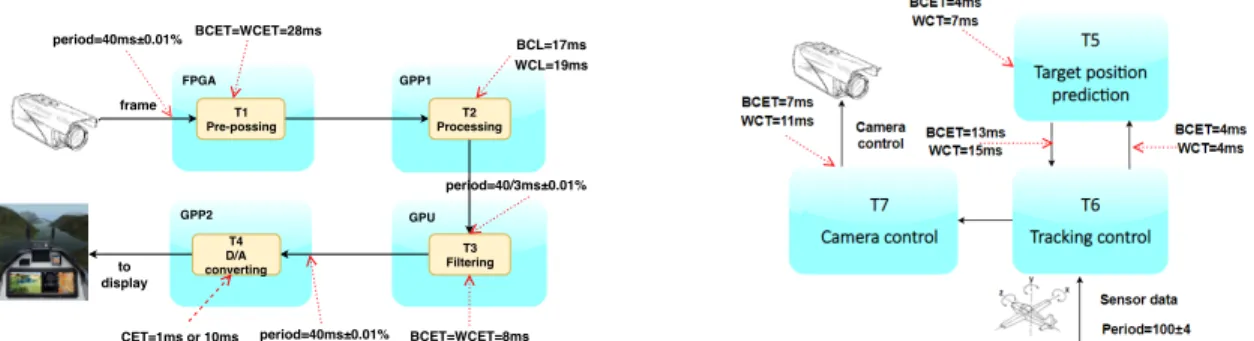
The FMTV 2015 challenge [8] consists of two subsystems, i.e., a video frame processing subsystem and a tracking & camera control subsystem.

T1 Pre-possing T2 Processing T3 Filtering T4 D/A converting to display frame period=40ms±0.01% BCET=WCET=28ms BCL=17ms WCL=19ms BCET=WCET=8ms CET=1ms or 10ms FPGA GPP1 GPU GPP2 period=40ms±0.01% period=40/3ms±0.01%

(a) The workflow of video frame processing subsystem (b) The workflow of the tracking and camera control subsystem

Fig. 4: Two subsystems in the FMTV 2015 Challenge 1) Aerial Video Frame Processing Subsystem: The first

challenge is a non-trivial scheduling problem in the aerial video frame processing system. In the system, there is a video frame processing chain to compute the timing latency for the frame processing and the timing distance separating two consecutive frame losses. Figure 4a shows the whole process. The process can be formalized as the following four tasks. 1) Pre-processing (T1): In this task, the frames are sent from

the camera with a period 40ms ± 0.01%. Triggered by the arrival of a frame, it will take 28ms to produce a new frame. 2) Processing (T2): The task takes the frame generated by task

T1 as input. The min (max) execution time is 17ms (19ms).

When finishing, a new frame is stored into the register. 3) Filtering (T3): This task is activated with a period of

40

3 ± 0.05% ms, and the execution time is 8 ms. In the

end, a new frame is stored in the buffer.

4) D/A converting (T4): This task is also activated with a

periodicity of 40 ± 0.01% ms. It takes 10 ms with a non-empty buffer, and at the end, a new frame will be displayed on the monitor, 1ms otherwise and without new frame. As an example, we only explain in the paper how task T4

is defined using parametric CCSL. The other three tasks can be defined likewise and we omit their definition details.

T4 s, T4 s1 + T4 s2 T4 s1# T4 s2

T_{4 f} , T4 f 1 + T4 f 2 T4 f 1 # T4 f 2

T4 f 1, T4 s1$ 1 on msec T4 f 2, T4 s2$ 3 on msec

T4 s, msec ./ 5 ± 1

From aforementioned, task T4is affected by the status of the

buffer. We declare four logical clocks T4 s1, T4 s2and T4 f 1, T4 f 2

to capture the start and end of the task in two conditions, i.e., the buffer is empty or nonempty. Because the buffer cannot be empty and nonempty simultaneously, the clocks must be exclusive, i.e., T4 s1# T4 s2 and T4 f 1 # T4 f 2. Furthermore, T4’s

period(40 ± 0.01%) can be modeled as periodicity of drift, denoted by T_{4 s}, msec ./ 5 ± 1.

T1 f ≡ T2 s T2 f ≡ T3 s1 (7a)

T4 s1 [3] ≺ T3 f 1 T3 f 1 ≺ T4 s1 (7b)

Task T2 and T3 are triggered by the arrival of the output

of tasks T1 and T2, and this synchronization pattern can be

captured as 7a. And 7b is used to formalize the buffer pattern and the data dependency between tasks T3 and T4.

Fig. 5: A schedule of task T2, T3 and T4 under bound 30

We encode the constraints into SMT formulas and analyze the satisfiability of the formulas using Z3. A schedule with bound 30 in Figure 5 is studied to shows the behaviors of tasks T2, T3 and T4.The history between the ith tick of clock T2 s

and T2 f is always 3, which satisfies the fixed execution time

constraint. When it comes to tasks T3and T4, they are the same

as task T2. Then the history between the two consecutive ticks

of T4 sare 5, 4, 4, which satisfies the constraint periodicity drift.

Furthermore, an execution sequence T2 s → T2 f → T3 s →

T3 s1 → T3 f → T3 f 1 → T4 s → T4 s2 → T4 f → T4 f 2 as

shown by the dashed arrows in the figure depicts the execution dependencies of the tasks T2, T3 and T4. It is a bounded

schedule which satisfies all the constraints.

2) Tracking and Camera Control Subsystem: For the cam-era tracking subsystem, it identifies objects on the camcam-era images and commands the camera motors so to follow the objects. This subsystem consists of 3 additional tasks: Task T6 is a periodic task with period P6= 100 and a certain drift

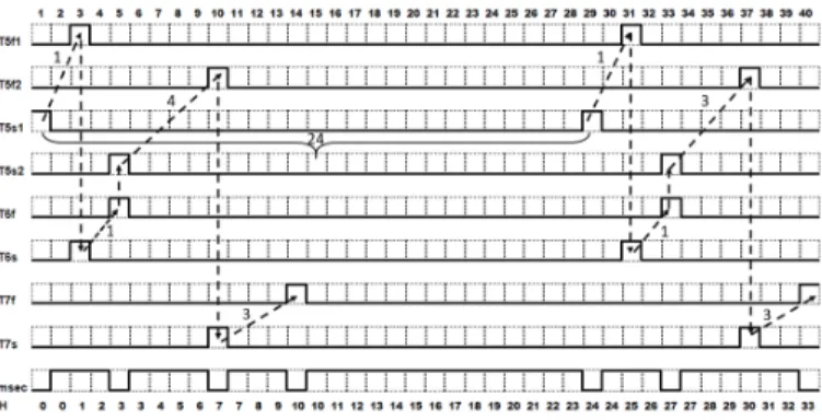
Fig. 6: A schedule of task T5, T6 and T7 under bound 40

call. Task T7 is activated synchronously by Task T6 and

con-trols the motors. Task T6 execution time is: C6,1= 4ms before

invoking Task T5; C6,2 ∈ [13, 15] ms after the completion of

Task T5 and before the invocation of Task T7. Task T7 has an

execution time of C7∈ [11, 14] ms. Here, the clock msec are

defined to tick for every 4 ms.

T5 f 1, T5 s1 $ 1 on msec T5 s1, msec ./ 25 ± 1

T5 f 2, T5 s2 $ p_p3 on msec p_p3 ∈ [3, 4]

For Task T 5, we declare four clocks T5s1, T5 f 1,T5s2, and

T5 f 2 to capture the start and finish of the first and second

parts of the task. The clocks satisfy the constraints above. Then, we transform the constraints into SMT formulas and solve them using Z3. Z3 returns one solution with bound 40. The schedule is shown in Figure 6. All the constraints can be proved to be satisfied by the solution.

C. Performance Evaluation

We study the efficiency of solving the encoded SMT formu-las in the two case studies. All the experiments were performed on Linux Mint 19 Cinnamon running on Intel© Xeon© CPU E5-1620 @3.60GHz×4 and 16GB memory. Table III shows the time that is taken by Z3 to return a result under different bound. One can see that there is an almost exponential increase of time, which corresponds to the NP-completeness of the scheduling problem of core CCSL [15]. Nevertheless, when the bound is small e.g., 40, we can obtain a result within reasonable time, which is still useful to analyze the constraints, particularly to detect inconsistencies in them.

V. Conclusion and Discussion

We proposed an approach of extending CCSL with param-eters and encoding the parametric CCSL into SMT formulas to model and verify the uncertainty-aware timing behaviors of embedded systems. Then we applied the approach to solving an opening timing verification problem for the industrial user-case proposed in the FMTV 2015 challenge.

Several approaches have been proposed to model uncer-tainties in real-time systems, e.g., parametric timed automata [16] and timed process algebra [10]. They rely on "physical-by nature" timings. Systems are presented as synchronously timed (a single global continuous time) and system events are constrained by value relations between physical clocks.

We are not trying to provide a competing approach. Instead, we make use of the flexibility of logical time and extend its

TABLE III: Execution time under different bound (s)

Bound Case Study 1 Case Study 2.1 Case Study 2.2 4/14/4 10/33/1 8/19/3 20 6.945 10.192 1.443 25 19.502 35.939 3.568 30 38.530 317.403 50.693 35 142.600 3024.993 114.717 40 420.606 43728.863 190.747 45 515.013 Time out 364.619 50 1557.640 Time out 910.096 55 1929.804 Time out 1485.992 60 4006.540 Time out 2118.655 65 8557.390 Time out 44257.193

1_{The 4/14/4, 10/33/1 and 8/19/3 indicate the number of clocks,}

constraints and parameters of each model, respectively.

expressiveness to cope with uncertainties. As the first step of modeling uncertainties using logical time, this work illustrates the possibility of linking physical time to logical time but raises more research problems such as the relationship between physical time models and logical time models. We believe that this work would inspire more work on studying problems in logical time scheduling using existing results of physical time scheduling, and vice versa.

Acknowledgments: This research was supported by Na-tional Key Research and Development Program of China (Grant No. 2018YFB2101300) and National Natural Science Foundation of China (Grant No. 61872146). Min Zhang is the corresponding author.

References

[1] F. Mallet and R. de Simone, “MARTE: a profile for RT/E systems modeling, analysis-and simulation,” pp. 1–8, 2008.

[2] C. André, F. Mallet, and R. De Simone, “Modeling time (s),” in IC on MODELS. Springer, 2007, pp. 559–573.

[3] J. Deantoni and F. Mallet, “TimeSquare: Treat your models with logical time,” in TOOLS’12. IEEE, 2012, pp. 34–41.

[4] Y. Ying and M. Zhang, “SMT-based approach to formal analysis of CCSL with tool support,” Ruan Jian Xue Bao/Journal of Software, vol. 29, no. 6, pp. 1595–1606, 2018.

[5] P. A. Laplante, “The certainty of uncertainty in real-time systems,” IEEE Instr.& Meas. Mag., vol. 7, no. 4, pp. 44–50, 2004.

[6] G. Lipari, “Real-time scheduling under uncertainty: Challenges and solutions,” in IC on EDiS. IEEE, 2017, pp. 227–227.

[7] L. M. de Moura and N. Bjørner, “Z3: An efficient SMT solver,” in TACAS’08, ser. LNCS, vol. 4963. Springer, 2008, pp. 337–340. [8] R. Henia and L. Rioux, “Formal methods for timing verification the

2015 FMTV challenge,” 2015.

[9] R. Alur and T. A. Henzinger, “Parametric real-time reasoning,” Cornell University, Tech. Rep., 1993.

[10] H.-H. Kwak, I. Lee, and O. Sokolsky, “Parametric approach to the specification and analysis of real-time scheduling based on ACSR-VP,” Science of Computer Programming, vol. 42, pp. 49–60, 2002. [11] R. Gregorian and G. C. Temes, “Analog mos integrated circuits for signal

processing,” New York, Wiley-Interscience, 1986, 614 p., 1986. [12] L. Lamport, “Time, clocks, and the ordering of events in a distributed

system,” Comm. ACM, vol. 21, no. 7, pp. 558–565, 1978.

[13] A. Benveniste, P. Caspi, S. A. Edwards, N. Halbwachs, P. Le Guernic, and R. de Simone, “The synchronous languages 12 years later,” Pro-ceedings of the IEEE, vol. 91, no. 1, pp. 64–83, 2003.

[14] F. Mallet and R. de Simone, “Correctness issues on MARTE/CCSL constraints,” Sci. of Comp. Prog., vol. 106, pp. 78–92, 2015.

[15] M. Zhang, F. Song, F. Mallet et al., “SMT-based bounded schedulability analysis of the clock constraint specification language,” in FASE’19, ser. LNCS 11424. Springer, 2019, pp. 61–78.

[16] T. Amnell, E. Fersman, L. Mokrushin, P. Pettersson, and W. Yi, “Times: A tool for schedulability analysis and code generation of real-time systems,” in FORMATS’03, ser. LNCS 2791. Springer, 2003, pp. 60–72.