Prediction of monsoon rainfall for a mesoscale Indian catchment based on stochastical downscaling and objective circulation patterns

(1)

HAL Id: hal-00298713

https://hal.archives-ouvertes.fr/hal-00298713

Submitted on 20 Sep 2005

HAL is a multi-disciplinary open access

archive for the deposit and dissemination of sci-entific research documents, whether they are pub-lished or not. The documents may come from teaching and research institutions in France or abroad, or from public or private research centers.

L’archive ouverte pluridisciplinaire HAL, est destinée au dépôt et à la diffusion de documents scientifiques de niveau recherche, publiés ou non, émanant des établissements d’enseignement et de recherche français ou étrangers, des laboratoires publics ou privés.

Prediction of monsoon rainfall for a mesoscale Indian

catchment based on stochastical downscaling and

objective circulation patterns

E. Zehe, A. K. Singh, A. Bárdossy

To cite this version:

E. Zehe, A. K. Singh, A. Bárdossy. Prediction of monsoon rainfall for a mesoscale Indian catchment based on stochastical downscaling and objective circulation patterns. Hydrology and Earth System Sciences Discussions, European Geosciences Union, 2005, 2 (5), pp.1961-1993. �hal-00298713�

(2)

HESSD

2, 1961–1993, 2005 Prediction of monsoon rainfall E. Zehe et al. Title Page Abstract Introduction Conclusions References Tables Figures J I J I Back Close

Full Screen / Esc

Print Version

Interactive Discussion

EGU Hydrol. Earth Sys. Sci. Discuss., 2, 1961–1993, 2005

www.copernicus.org/EGU/hess/hessd/2/1961/ SRef-ID: 1812-2116/hessd/2005-2-1961 European Geosciences Union

Hydrology and Earth System Sciences Discussions

Papers published in Hydrology and Earth System Sciences Discussions are under open-access review for the journal Hydrology and Earth System Sciences

Prediction of monsoon rainfall for a

mesoscale Indian catchment based on

stochastical downscaling and objective

circulation patterns

E. Zehe1, A. K. Singh2, and A. Bardossy3

1

Institute of Geoecology, University of Potsdam, Germany

2

Civil Engineering Department, Nirma University of Science and Technology (NU) Ahmedabad 382 481, India

3

Institute of Hydraulic Engineering, University of Stuttgart, Germany

Received: 15 July 2005 – Accepted: 1 September 2005 – Published: 20 September 2005 Correspondence to: E. Zehe ([email protected])

(3)

HESSD

Full Screen / Esc

Print Version

EGU Abstract

In this study a stochastical approach for generating rainfall time series based on ob-jective circulation patterns (CP ) is applied to the mesoscale Anas catchment in North West India. This CP based approach was developed and successfully applied in the humid and temperate climate of Central Europe. The objective of the study was to find

5

out whether this approach is transferable to a catchment in North West India with a to-tally different semi arid climate. For the Anas catchment it was possible to identify a CP classification scheme consisting of 12 CP s defined in a window between 5◦N40◦E and 35◦N95◦E, which explained the space-time variability of observed rainfall at 10 stations in the Anas catchment. Based on the classification scheme, NCAR pressure data from

10

500 hPa level were classified into a CP time series for the period of 1964–1994, which was in turn used as meteorological forcing for multivariate stochastical rainfall simu-lations with a daily time step. On the monthly time scale the model performed well. Except for stations Udaigarh and Bhabra the average annual cycle of monthly rainfall and rainy days in a month was matched well. The frequency distributions of monthly

15

rainfall at different stations were also captured well. Correlation coefficients between simulated and observed monthly rainfall were larger than 0.85 at each station. Within a long term simulation of 30 years the model yielded promising predictions for monthly as well as for seasonal rainfall totals, but showed also clear deficiencies in capturing the very extremes and inter-decadal variability of monsoon strength. In this respect, the

20

introduction of additional predictors such as SST anomalies and wind direction classes promised the most substantial model improvements.

1. Introduction

The strong seasonality of the Indian climate and especially the onset and strength of the rainy season determines to a high degree the socio-economic development and

25

(4)

HESSD

Full Screen / Esc

Print Version

EGU than 50% of its land area (MoE 2004). With 2/3 of the Indian population depending

on agriculture for employment and 2/3 of the cultivated land relying on rainfed farming, water and food security closely follow climate variability and extremes. Thus, seasonal predictions of the onset and strength of monsoon rainfall are crucial for water resources as well as agricultural management and planning in India (Webster and Hoyos, 2004;

5

Siddiq, 1999). During the monsoon season, usually from June to September, the In-dian subcontinent receives 80–90% of the total annual rainfall in a sequence of rainy periods (monsoon bursts) and dry periods (monsoon breaks) of 10–20 days duration, which seem to occur quite randomly (Webster and Hoyos, 2004). Different methods for predicting inter seasonal variability of monsoon rainfall over the Indian subcontinent

10

have been proposed over the years. Shukla and Mooley (1987) used the EL Ni ˜no Southern Oscillation (ENSO) to explain 30% of the temporal monsoon variability over the Indian subcontinent. Early attempts to statistically link Eurasion snow fall in winter to the strength of the Indian monsoon did not yield convincing results (Dickson, 1984; Bamzai and Shukla, 1999). Harzallah and Sadourny (1999) and Clarke et al. (2000)

15

proposed empirical schemes for linking monsoon rainfall and sea surface tempera-ture anomalies. Gowarikar et al. (1991) developed a regional scale power regression models for rainfall forecasting in selected regions of India based on a time domain approach.

Despite the importance of large scale seasonal predictions of Indian monsoon, the

20

question of how climate change will affect the spatio-temporal pattern of monsoon rain-fall and the related hydrological impact in mesoscale river basins is of high interest. The assessment of climate change impact on monsoon rainfall for mesoscale river basins requires approaches that may be linked to climate scenarios generated with Global Cir-culation Models (GCMs). This link might be achieved either by dynamical or empirical

25

downscaling (Wilby and Wilks, 1997).

Within the dynamic approach, a “cascade” of dynamic models run on a nested grid, where the finer resolved, regional models are driven by a Global Circulation Model (GCM). Regional models may be either regional climate models (Giorgi et al., 1998;

(5)

HESSD

Full Screen / Esc

Print Version

EGU Frei et al., 1998; Jacob et al., 2001; Bergstr ¨om et al., 2001), which are hydrostatic

models, or non hydrostatic mesoscale weather forecasting models such as the MM5 (Kunstmann and Jung, 2003). Dynamical downscaling yields satisfactory results when driven by GCMs in the assimilation mode. However, even when the same GCM forcing is used within a climate change scenario, regional climate models (RCMs) may produce

5

significantly different results as recently shown by Jacob et al. (2001) in a comparative study for the Baltex area involving several different RCMs.

The basic idea of the empirical approach is firstly to establish a functional relationship between the most robust and reliable fields provided by GCMs, such as geo-potential height and temperature and locally observed meteorological variables such as

precip-10

itation or temperature in the catchment of interest, and secondly to extrapolate into the future based on the GCM scenarios assuming the functional relationship is station-ary. Within empirical downscaling we distinguish methods which directly link the GCM predictors to the surface variables in a basin of interest, resampling methods (W ´ojcik and Buishand, 2003) or methods based on weather types. “Expanded Downscaling”

15

(EDS) proposed by B ¨urger (2002) is a good example of a direct method. The principle is to predict catchment scale precipitation and temperature using a multivariate regres-sion model with the geo-potential height, the temperature and the specific humidity of the GCM as predictors. The important constraint is that for the present climate, the observed spatial correlation structure of the surface variables has to be maintained.

20

Similarly, Wilby et al. (1999) used sea level pressure, the geo-potential height of the 500 hpa pressure level and relative humidity to model daily rainfall within a regression model.

Weather type related approaches are based on the assessment of weather types or circulation patterns, which are statistically linked to the target surface variables in

25

the basin of interest (Wilson et al., 1992, Bardossy et al., 1995; Wilby and Wigley, 2000; Conway and Jones, 1998; ¨Ozelkan et al., 1998). Stehlik and B ´ardossy (2002) suggested an approach for relating large scale atmospheric pressure data and basin scale precipitation based on:

(6)

HESSD

Full Screen / Esc

Print Version

EGU – An optimisation of fuzzy rules to classify pressure data from a suitable spatial

window into a number of circulation patterns (CP s), to explain the basin scale space-time variability of observed rainfall.

– A multivariate stochastical generation of rainfall data at different locations in the

basin using rainfall probabilities and a spatial correlation both conditioned to the

5

CP s obtained with the optimised classification scheme. In contrary to unisite approaches, the method allows estimation of precipitation with a realistic spatio-temporal pattern.

As the output of climate models maybe classified into CP time series too, the method is suitable for quantifying climate change impact on catchment scale precipitation. For

10

simulating precipitation in the 14 000 km2 large Neckar basin in Germany, a set of 12 different CP s turned out to be optimal, which where classified using sea level pressure data (SLP) with a spatial resolution of 5◦ from a window with South-West and North-East corners located at 35◦N, 15◦W and 65◦N, 40◦E, respectively. In the following, we will refer to this method as the CP based approach for precipitation downscaling.

15

The objective of the present study is to shed light on whether the CP based ap-proach, which was developed and successfully applied to quantify climate change im-pact on catchment scale rainfall in the humid and temperate climate of Central Europe, is transferable to a catchment in North West India with a totally different semi arid cli-mate that is strongly affect by the seasonality of the Indian Ocean circulation. Specific

20

aims are:

– To shed light on how well we can predict monthly totals of monsoon rainfall as well

as inter-annual variability of monsoon strength and onset,

– To identify model deficiencies and discuss additional predictors which are

orthog-onal to atmospheric pressure patterns to potentially improve the model

perfor-25

(7)

HESSD

Full Screen / Esc

Print Version

EGU To this end we had to identify an optimal location for the pressure window and an

optimum number of circulation patterns. The next section will give a brief outline of the downscaling methodology, the study area as well as the underlying database.

2. Methodology and study area

2.1. Downscaling methodology

5

2.1.1. Fuzzy rule based classification of circulation patterns

As a first step the geo-potential heights of pressure data from a suitable pressure level such as 500 hPa or SLP (sea level pressure) are transformed to standardised anoma-lies by subtracting the long term average from the actual value at each node and di-viding the resulting difference by the long term standard deviation. Based on triangular

10

fuzzy membership functions the daily anomalies at each location (x, y) are classified into the categories 1) high, 2) medium high, 3) medium low, 4) low or 5) indifferent for the circulation pattern. The membership functions for the five categories are v=1, low: (−2.0, −1, −0.2)_T; v=2, medium low: (−1.4, −0.6, 0)_T; v=3, medium high: (0, 0.6, 1.4)_T; v=4, very high: (0.2, 1, 2.0)_T; and v=5, constant as 1. Thus a circulation

15

pattern, CP_k, is fully characterised by an index vector v (k)={v(1)(k)...v (n)(k)} that defines the location of heights and depressions in the pressure window according to four categories as well as those nodes which are of no importance i.e. which belong to category 5. A pressure pattern for a given day is classified into a circulation pattern by calculating the degree of fulfilment (DOF) for each rule based on the membership

val-20

ues, µ, of the actual pressure anomaly value at each node in the window and selecting the CP with the highest DOF (B ´ardossy et al., 2002).

The next step is to define a suitable objective function for the optimisation procedure based on available precipitation time series in the basin. Following the approach of

(8)

HESSD

Full Screen / Esc

Print Version

EGU Stehlik and B ´ardossy (2002) we defined:

O₁= S X i=1 v u u t 1 N_d Nd X t=1 (p(CP (t))_i − ¯p)2 (1)

where S is number of stations with precipitation observations, N_d is the number of days in the time series, p(CP (t))_i is the CP -conditional probability of a wet day at station i, ¯p_i is the total average probability at station i . High values of O₁ indicate that

5

the conditional rainfall probabilities of the CP s differ strongly from the average value i.e. represent dryer or wetter than average meteorological conditions for the basin. Stehlik and B ´ardossy (2002) propose a second objective O₂based on the conditional precipitation amounts z(CP ): O₂= S X i=1 1 N_d Nd X t=1 log z_p(CP (t))_i ¯ z_p,i ! (2) 10

where ¯z_i is the overall average daily precipitation amount at station i . High values of O₂ indicate that the conditional rainfall amount of a CP differ clearly from the average value. Following Stehlik and B ´ardossy (2002), we used the sum of O₁ and O₂ as one possible objective function O for CP optimisation. Alternatively we defined an objective function O

0

2 based on the conditional precipitation amounts z(CP ) which gives more

15

emphasis on CP with very high/low daily rainfall amounts

O₂= S X i=1 1 N_d Nd X t=1 z(CP (t))_i z_i !b (3)

The total objective function, O0, was again the sum of O₁and O

0

2, 1 and 1.5 were tested

as a possible exponent b.

For optimisation we use simulated annealing. The principle of the optimisation is

20

(9)

HESSD

Full Screen / Esc

Print Version

EGU based on the observed precipitation time series. Then a rule k is randomly selected

and one of the five categories, v , is randomly assigned to a randomly chosen location, x_i, y_i. A new classification is performed and O∗ is calculated. If O ∗ >O then the change is accepted, if not the change is accepted with a probability that decreases with decreasing annealing temperature. More details on the optimisation are given in

5

B ´ardossy et al. (2002).

Within the present study, the following classification schemes were optimised: a set of 8, 10 or 12 CP s, classified from geo-potential heights of the 500 HPa pressure level from two possible windows; one with South-West and North-East corners located at 5◦N 40◦E and 35◦N 95◦E (Fig. 1) the other located between 0◦N 45◦E and 30◦N

10

100◦E. Furthermore we compared the objective functions, O and O0, for possible expo-nents of b=1, 1.5.

The objective function itself is a good criterion to compare the quality of different CP classification schemes. In addition we used the following measures:

– The normalised rainfall probability, n_p, defined as the conditional probability of

15

precipitation at station i given the condition that the pressure at a day is classified into a given CP divided by the average precipitation probability, ¯p_i, at this station. A strong deviation of n_pfrom 1 indicates that the conditional rainfall probability of the CP is much higher or lower than the average.

n_p= pi(CP ) p_i 20

– The normalised rainfall amount, n_z, defined as the conditional average precipita-tion amount on a wet day for a given CP z_i(CP ) at station i divided by the average precipitation amount, ¯z_i, of a wet day at that station. A strong deviation of n_z from 1 indicates that the conditional rainfall amount of the CP is much higher or lower

(10)

HESSD

Full Screen / Esc

Print Version

EGU than the average:

n_z= zi(CP ) z_i

– The wetness index, I_wet, defined as product of n_pand n_z. 2.1.2. Stochastical precipitation model

The time series of classified circulation patterns represents the large scale forcing of a

5

model originally proposed by B ´ardossy and Plate (1995) and advanced by Stehlik and B ´ardossy (2002). It is a conditional multivariate autoregressive rainfall model based on a transformed multivariate normal distribution. Rainfall is linked to the individual CP using conditional rainfall probability and amounts. Spatial covariance of daily precipita-tion is a funcprecipita-tion of the actual CP as well as of the day in the year. The annual cycles

10

of the spatial covariance function and of the one day lag autocorrelation are described by means of a Fourier series. Stehlik and B ´ardossy (2002) showed that the first three harmonics are sufficient for describing the annual cycles of the autocorrelation as well as of the spatial covariance of rainfall. As Stehlik and B ´ardossy (2002) provide very detailed information on the precipitation model as well as on the estimation of model

15

parameters we omit further details here. The model was calibrated using a period of 10 years (1985–1994) of precipitation data from 10 stations in the study area.

2.2. Study area and database

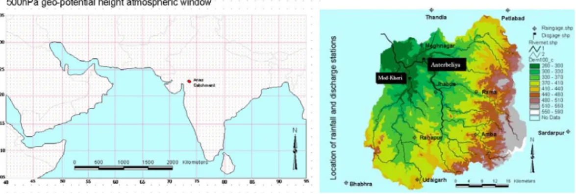
The Anas catchment is a head watershed of the Mahi basin which falls under a semi-arid climatic zone in western India (Fig. 1). The catchment covers a geographical

20

area of 1750 km2 with a mean altitude ranging from 280 m to 560 m. Daily rainfall data records for 10 stations were provided from the State Water Data Centre (SWDC) at Bhopal. The average daily rainfall amount, the observed maximum, the standard deviation and the skewness of the time series at the 10 stations are listed in Table 1.

(11)

HESSD

Full Screen / Esc

Print Version

EGU The total rainfall in the monsoon season which provides 90% of the total annual rainfall

ranges from 350 mm to 1300 mm for dry to wet years, respectively. The rainfall station at Jhabua has the longest records ranging from 1957–1999. Records at Thandla range from 1964–1999 and the data records at the remaining stations range from 1984–1999. Hence, we selected the period from January 1985 to December 1994 for optimising the

5

CP classification scheme. Since 80–90% of the rainfall falls during monsoon season which ranges usually from June to October, rainfall data were only collected during the monsoon season. Consequently, conditional rainfall probabilities and amounts for the CP s were exclusively determined for the monsoon period and set to zero outside.

For the optimisation of the CP classification we used a geo-potential height of the

10

500 hPa pressure level provided by the National Meteorological Centre for Atmospheric Research (NCAR) on a 5◦ by 5◦grid for the two windows specified above (Fig. 1).

3. Results

3.1. Optimal CP classification scheme

Table 2 compares the different classification schemes in terms of the two CP s that

15

have the maximum and minimum values of the normalised precipitation probability and normalised precipitation amount. A total number of 12 CP s allows the best explanation of rainfall variability because the conditional precipitation probability and amount of the wettest and driest CP s deviate stronger from the average values than for the schemes based on 10 and 8 CP s. Hence, the classification scheme with 12 CP s is superior

20

for explaining extremely wet or dry meteorological conditions. For the same reasons, the window with South-East and North-West corners located 5◦N 40◦E and 35◦N 95◦E gives better results than the window located between 0◦N 45◦E and 30◦N 100◦E. The comparison of the different objective functions, O₂ and O0₂, suggests that O0₂with an exponent of b=1 gives the best results. Thus we may state that the classification

25

(12)

HESSD

Full Screen / Esc

Print Version

EGU when optimised with objective function O₂’ and with b=1.

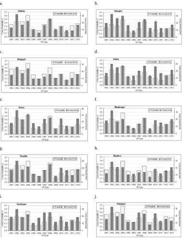
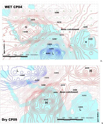
Figure 2 presents the conditional rainfall probability and amounts for the 12 CP s and for each station in the Anas catchment. CP4, CP3, CP2 and CP8 represent wet meteorological conditions. On average, CP4 is the wettest due to the highest average wetness index. Due to a depression located over the Indian Ocean and a strong

an-5

ticyclone with its centre over the Arabian island, CP4 causes a streaming of moist air masses from the North Western Indian Ocean to North Western India (Fig. 3). CP5, CP11, CP13 and CP9 represent dry conditions, e.g. the dry CP9 with a “bridge” of two anticyclones ranging from the Indian Ocean to Mongolia which causes dry and hot weather conditions.

10

3.2. Stochastical rainfall simulation

3.2.1. Model performance at the daily time scale

Table 4 lists simulated and observed averages and standard deviations of seasonal rainfall as well as the average number of rainy days for all stations in the Anas catch-ment, calculated for the period 1985–1994. The deviations between the moments and

15

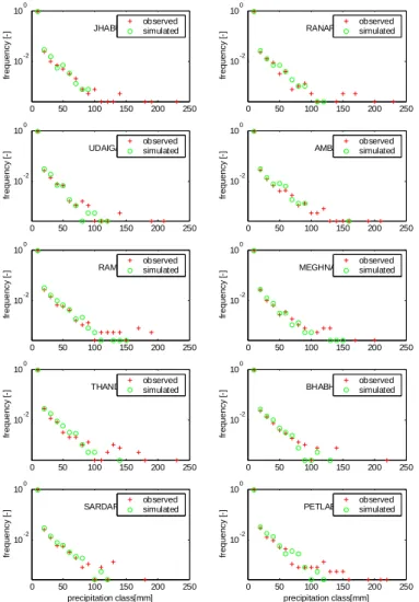
the number of rainy days are entirely within the 95% confidence intervals. The compari-son between the histograms of observed and simulated daily rainfall (Fig. 4) suggests a good agreement for rainfall amounts falling in the lower 99.5% percentile. However, the model systematically underestimates the occurrence of the extremes within the upper 0.5% percentile. For each station, we tested whether the histograms of simulated and

20

observed rainfall time series belong to the same distribution for a significance level of 95% by means of a chi-squared test. For stations Thandla and Petlabad the hypothesis had to be rejected.

(13)

HESSD

Full Screen / Esc

Print Version

EGU 3.2.2. Model performance at the monthly time scale

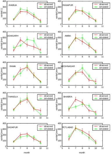
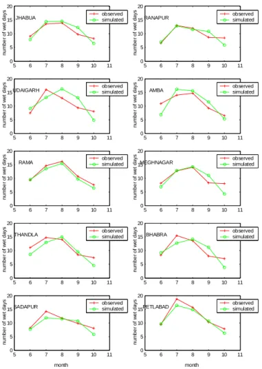
Except for the stations Udaighar and Bharba, which are located in the South West of the Anas catchment, the model results match the average annual cycles of monthly rainfall and rainy days well (Figs. 5 and 6). At both stations the model underestimates rainfall in July and overestimates in the second half of the monsoon period. As shown

5

in Fig. 6, this is because of a corresponding mismatch of simulated and observed rainy days, underestimation in July and overestimation in the period of August–October.

The correlation between observed and simulated monthly rainfall totals is good, with values larger than 0.85 (Table 5). As shown by the histograms of observed and sim-ulated monthly rainfall, the model captures the occurrence of extremes clearly better

10

than at the daily scale. Again we tested whether the histograms of simulated and ob-served rainfall time series belong to the same distribution for a significance level of 95%. The hypothesis was accepted for each station.

3.2.3. Long term monsoon prediction

To test the model performance outside of the calibration period, monsoon rainfall time

15

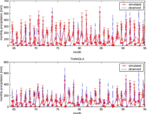
series were simulated for the period from 1964-94 and compared to the observations at stations Thandla and Jhabua, where long term series are available. Due to the stochastic nature of the model, we generated 30 realizations of rainfall time series and computed time series of monthly and rainfall seasonal by averaging over the re-alizations. The uncertainty band of the simulated rainfall series is marked by the 95%

20

confidence intervals around the average value. At both stations Thandla and Jhabua, the model yields reasonable long term predictions of monthly rainfall (Fig. 8). Correla-tion coefficients between observed and simulated monthly rainfall are 0.51 and 0.59. However, the model clearly underestimates the extremes in the years 1988 and 1993. Figure 9 presents simulated and observed time series for the seasonal totals of

25

monsoon rainfall at both stations. The correlation coefficients between simulated and observed seasonal totals at Thandla and Jhabua are 0.62 and 0.48, respectively. At

(14)

HESSD

Full Screen / Esc

Print Version

EGU the Thandla station the model clearly underestimates monsoon rainfall in the period of

1969 to 1982. In the following period from 1983–1994 (calibration period 1985–1994) and no systematic underestimation is observed. The normalized difference between simulated and observed cumulated rainfall totals in the simulation period is −0.19, which is outside of the 95% confidence limit of the observed total rainfall. A possible

5

reason for the different types of model errors in the periods of 1969–1982 (negative bias) and 1983–1992 (statistical error) could be inter-decadal variability of monsoon strength.

In contrary, at the Jhabua station, no period of systematic model error or bias may be identified. The normalized difference between simulated and observed cumulated

10

rainfall totals in the simulation period is with −0.04 inside the 95% confidence limit of the observed rainfall.

4. Discussion and conclusions

The results presented suggest that the CP based approach for precipitation downscal-ing, which was originally developed by Stehlik and B ´ardossy (2002) and successfully

15

applied in the humid and temperate climate of Central Europe, is applicable within the totally different, semi arid climate of North West India. The optimal classifica-tion scheme consists of a set of 12 CP s defined in a window between 5◦N 40◦E and 35◦N95◦E. Within the optimisation procedure, a modified objective function, O0₂(Eq. 3), which gives higher weights to days with higher rainfall, yielded better results than the

20

O₂(Eq. 2), which was originally proposed by B ´ardossy et al. (2002).

Based on the classification scheme, NCAR pressure data from 500 hPa level were classified into a CP time series for the period of 1964–1994, which was in turn used as meteorological forcing for multivariate stochastical rainfall simulations with a daily time step.

25

On the monthly time scale the model performed well inside the calibration period and also yielded promising predictions outside the calibration period. Except for stations

(15)

HESSD

Full Screen / Esc

Print Version

EGU Udaigarh and Bhabra, the average annual cycle of monthly rainfall and rainy days in

a month was matched well. Both stations are located at the South-West of the Anas regions. The wettest CP4 (Fig. 3), which dominates in the early monsoon period, causes streaming of humid air masses from North West into the Anas region. In this case, Udaigarh and Bhabra are at luv side of mid mountains. Thus, topographic effects

5

will cause stronger rainfall, which is obviously not captured by the stochastical model. In the second part of the monsoon period, the wet CP2 dominates, which causes streaming of moist air mass from South West. In this case, Udaigarh and Bhabra are at the lee side of mid mountains, which will cause weaker precipitation, which is again not captured by the model. A possible way to account for this effect of advection

10

and topography is to introduce conditional rainfall probabilities and amounts which are conditioned by the CP and the classes of wind direction and strength.

Within a long term simulation of 30 years, the model yielded promising predictions for monthly as well as for seasonal rainfall totals. The model explained on average between 25% and 36% of the observed rainfall variability. The model is suitable

15

for explaining parts of the intra seasonal monsoon variability as well as parts of the inter-seasonal variability of monsoon rainfall, as recommended by Webster and Hoyos (2004). However, model simulations at the Thandla station showed a negative bias of nearly 20% due to a systematic underestimation of monsoon rainfall in the period 1969–1982. In contrary, the model simulations were unbiased in the period 1983–1992,

20

which covered the calibration period. This is likely to be due to inter-decadal variability of monsoon strength, which is a well known phenomenon. Shukla and Mooley (1987) already showed that the EL Ni ño Southern Oscillation (ENSO) has a strong influence on monsoon performance: El Ni ño coincides with low monsoon performance whereas La Ni ña causes stronger monsoon seasons (Webster and Hoyos, 2004; Goddard et

25

al., 2003). Furthermore, Clarke et al. (2000), Clarke and Webster (1999), Hastenrath (1987) as well as Harzallah and Sadourny (1999) report that the sea surface temper-ature (SST) of the Indian Ocean influences the inter-decadal variability of monsoon strength. The most straight forward way to introduce SST anomalies as additional

(16)

HESSD

Full Screen / Esc

Print Version

EGU predictors into the stochastic rainfall model we used here is to define conditional

rain-fall probabilities and amounts which are conditioned by the CP as well as by the SST anomalies in the Indian Ocean. Due to the slow variation of STT this would require longer calibration periods up to 20 years. The main difficulties within this context are

– To identify the “sensitive” area in the India Ocean at which SST anomalies are

5

important

– To better understand whether SST anomalies in a certain sensitive area is

impor-tant or whether the spatial pattern, consisting of SST highs and lows (similar to a circulation pattern) determines the inter-decadal variability of monsoon strength. The over all conclusion of this study is that the CP based approach for precipitation

10

downscaling, proposed by Stehlik and B ´ardossy (2002) is applicable for monthly pre-dictions of monsoon rainfall in the semi arid climate of North West India. Since the geo-potential height of GCM pressure fields can also be classified into CP time series, the method allows, in principle, impacts of climate changes scenarios on Indian mon-soon for mesoscale catchments to be quantified. As discussed above the following

15

developments promise substantial model improvement:

– Introduction of conditional rainfall probabilities and amounts which are conditioned

by the CP and classes of wind direction and strength to better account for advec-tion of precipitaadvec-tion and topographic effects (luv/lee). We expect this to improve the model within the monsoon season

20

– Introduction of conditional rainfall probabilities and amounts which are conditioned

by the CP as well as by the SST anomalies or by patterns of SST anomalies in the Indian Ocean. We expect this to improve the model performance in capturing inter seasonal and inter-decadal variability of monsoon total rainfall.

(17)

HESSD

Full Screen / Esc

Print Version

EGU References

B ´ardossy, A., Stehlik, J., and Caspary, H.-J.: Automated objective classification of daily circula-tion patterns for rainfall and temperature downscaling based on optimised fuzzy rules, Clim. Res., 23, 11–22, 2002.

B ´ardossy, A., Stehlik, J., Caspary, H.-J.: Generating of areal precipitation series in the upper

5

Neckar catchment, Phys. Chem. Earth (B), 26, 683–687, 2001.

B ´ardossy, A., Duckstein, L., and Bog ´ardi, I.: Fuzzy rule based classification of atmospheric circulation patterns, Int. J. Climatol., 15, 1087–1097, 1995.

B ´ardossy, A. and Plate, E. J.: Space-time model of daily rainfall using atmospheric circulation patterns, Water Resour. Res., 28, 5, 1247–1259, 1992.

10

Bamzai, A. S. and Shukla, J.: Relation between Eurasian snow cover, snow depth and the Indian summer monsoon: An observational study, J. Clim., 12, 3117–3132, 1999.

Bogardy, I., Matyasovszky, I., Bardossy, A., and Duckstein, L.: A hydro-climatological model of areal droughts, J. Hydrol., 153, 245–264, 1994.

Brandsma, T. and Buishand, T. A.: Statistical linkage of daily precipitation in Switzerland to

15

atmospheric circulation and temperature, J. Hydrol., 198, 98–123, 1997.

Bergstrom, S., Carlson, B., Gardekin, M., Lindstrom, G., Peterson, A., and Rummukainen, M.: Climate change impacts on Hydrology in Sweden – assessment by global circulation models, dynamical downscaling and hydrological modelling, Clim. Res., 16, 101–112, 2001.

Booij, M. J.: Appropriate modelling of climate change impacts on river flooding, PhD.-thesis,

20

Univ. of Twente, Twente, 206 pp., 2001.

B ¨urger, G.: Selected precipitation scenarios across Europe, J. Hydrol., 262, 99–110, 2002. Clark, C. O., Cole, J. E., and Webster, P. J.: Indian ocean SST and Indian summer rainfall:

Predictive relationships and their decadal variability, J. Clim., 13, 2503–2519, 1999.

Clarke, M. P., Hay, L. E., McCabe, G. J., Leavesley, G. H., Serreze, M. C., and Wilby, R.

25

L.: The use of weather and climate information in management of water resources in the western United States. Proceedings of the Special Conference on Climate Variability and Water Resources, NOAA, Boulder, USA, 2001.

Clark, C. O., Cole, J. E., and Webster, P. J.: SST and Indian summer rainfall: Predictive rela-tionships and their decadal variability, J. Clim., 13, 2503–2519, 2000.

30

Christensen, J. H., Machenhauer, B., Jones, R. G., Sch ¨ar, C., Ruti, P. M., Castro, M., and Visconti, G.: Validation of present-day climate simulations over Europe: Lam simulations

(18)

HESSD

Full Screen / Esc

Print Version

EGU with observed boundary conditions, Clim. Dynam., 13, 489–506, 1997.

Conway, D. and Jones, P. D.: The use of weather types and airflow indices for GCM downscal-ing, J. Hydrol., 213, 348–361, 1998.

Cubash, U., Waszkewitz, J., Hegerl, G., and Perlwitz, J.: Regional climate change as simulated in time-slice experiments, Clim. Change, 31, 273–304, 1995.

5

Dickson, R. R.: Eurasion snow cover versus Indian monsoon rainfall, An extension of the Hahn-Shukla results, J. Climate Appl. Meteor., 23, 171–173, 1984.

DWC: Climate changes and water rules, Dialogue on water and climate, Delft, The Netherlands, 2003.

Frei, C., Schar, C, Luthi, D, and Davies, H. C.: Heavy precipitation processes in a warmer

10

climate, Geophys. Res. Lett., 25, 1431–1434, 1998.

Giorgi, F. , Mearns, L. O., Shields, C., and McDaniel, L.: Regional nested model simulations of present and 2×CO₂climate over the central plains of the US, Clim. Change, 40, 457–493, 1999.

Giorgi, F.: Perspectives for regional earth system modelling, Global Planet. Change, 10, 23–42,

15

1995.

Gregory, J. M. and Mitchel, J. F. B.: Simulation of daily variability of surface temperature and precipitation over Europe in the current and the 2×CO2 climates using the UKMO climate

model, Q. J. Royal Meteor. Soc., 121, 1451–1476, 1995.

Gowarikar, V., Thapliyal, V., Sarkar, R. P., Mandal, G. S., Sen Roy, N., and Sikka, D. R.:

Param-20

eteric and power regression models: New approach to long range forecasting of monsoon rainfall in India, Mausam, 40, 115–122, 1989.

Gowarikar, V., Thapliyal, V., Kulshrestha, S. M., Mandal, G. S., Sen Roy, N., and Sikka, D. R.: A power regression model for long range forecast of south-west monsoon rainfall over India, Mausam, 42, 125–130, 1991.

25

Harzallah, A. and Sadourny, R.: Observed lead lag relationships between Indian summer mon-soon and some meteorological variables, Climate Dyn., 13, 635–648, 1999.

Hulme M.: An intercomparision of model and observed global precipitation climatologies, Geo-phys. Res. Lett., 18, 1715–1718, 1991.

IPCC: Climate change- impacts, adaptation and vulnerability, 3rd Assessment Report of the

30

Intergovernmental Panel on Climate Change, Cambridge University Press, UK, 2001. IPCC: The regional impacts of climate change – an assessment of vulnerability, Assessment

(19)

HESSD

Full Screen / Esc

Print Version

EGU 1998.

Jones, R. G., Murphy, J. M., and Noguer, M.: Simulation of climate change over Europe using a nested regional-climate model I. assessment of control climate, including sensitivity to location of lateral boundaries, Q. J. Royal Meteor. Soc., 121, 1413–1449, 1995.

Jacob, D., B ¨ulow. K., and Milliez, M.: Dynamische und statistische Erstellung

5

von hochaufgel östen Klimaszenarien (1/6◦) als Basis f ür wasserwirtschaftliche Hand-lungsempfehlungen im KLIWA-Projekt B 1.1.1 Klimaszenarien, Max-Planck-Institut f ür Me-teorologie, Hamburg, Germany, 2003.

Jacob, D., van den Hurk, J. J. M., Andrae, U., Elgered, G., Fortelius, C. Graham, L. P., Jackson, S, D., Karstens, U., K ¨opken, Chr. Lindau, R. Podzun, R., Rockel, B. Rubel, F. Sass, B. H.,

10

Smith, R. N. B., and Yang, X.: A comprehensive model inter-comparison study investigating the water budget during the BALTEX-PIDCAP period, Meteorol. Atmos. Phys., 77, 19–43, 2001.

Kunstmann, H. and Stadler, C: Coupled high resolution meteorological-hydrological simulations for the alpine catchment of the river Mangfall, Hydrologie und Wasserbewirtschaftung, 47, 4,

15

151–159, 2003.

Kunstmann, H. and Jung, G.: Investigation of feedback mechanisms between soil moisture, landuse and precipitation in West Africa. Water Resources System, Water Availiability and Global Change, IAHS Publications, 280, 159–159, 2003.

MoE India: India’s National Communication of the UNFCCC, Ministry of Environment and

20

Forests, Government of India, Delhi, 2004. ¨

Ozelkan, E., Galambosi, Duckstein, L., and B ´ardossy, A.: A multi-objective fuzzy classifica-tion of large scale circulaclassifica-tion patterns for precipitaclassifica-tion modeling, Applied Mathematics and Computation, 91, 127–142, 1998.

Shukla, J. and Mooley, D. A.: Empirical prediction pf the summer monsoon rainfall over India,

25

Mon. Wea. Rev., 115, 695–703, 1997.

Siddiq, E. A.: Rainfall prediction for rice growing areas, in: Rice in a variable climate, edited by: Abrol, Y. P. and Gadgilm S., APC Publication Delhi, 107–123, 1999.

Stehlik, J. and Bardossy A.: Multivariate stochastic downscaling model for generating daily Rainfall series based on atmospheric circulation, J. Hydrol., 256, 120–141, 2002.

30

Webster, P. J. and Hoyos, C.: Prediction of monsoon rainfall and river discharge on 15-30 day time scales, Bull. Amer. Meteor. Soc., 85, 1745–1767, 2004.

(20)

resam-HESSD

Full Screen / Esc

Print Version

EGU pling schemes, J. Hydrol., 273, 69–80, 2003.

Wilby, R. L. and Wigley, T. M. L.: Precipitation predictors for downscaling – observed and general circulation model relationships, Int. J. Climatol., 20, 641–661, 2000.

Wilby, R. L, Hay, L. E., and Leavesly, G. H.: A comparsion of downscaled and raw GCM output: implications for climate change scenarios in the San Juan River basin, Colorado, J. Hydrol.,

5

225, 67–91, 1999.

Wilby, R. L., Wigley, T. M. L., Conway, D., Jones, P. D., Hewitson, B. C., Main, J., and Wilks, D. S.: Statistical downscaling of general circulation model output: A comparison of methods, Water Resour. Res., 34, 11, 2995–3008, 1998.

Wilby, R. L. and Wigley, T. M. L.: Downscaling general circulation model output: a review of

10

methods and limitations, Prog. Phys. Geogr., 21, 530–548, 1997.

Wilson, L. L., Lettenmaier, D. P., and Skyllingstaed, E.: A multiple stochastic daily precipitation model conditional on large scale circulation patterns, J. Geophys. Res., 97, 2791–2801, 1992.

(21)

HESSD

Full Screen / Esc

Print Version

EGU

Table 1. Statistical properties of daily rainfall data for various stations of the Anas catchment

during the monsoon season.

Station Average (mm) Maximum (mm) Standard deviation (mm) Skewness (–)

Jhabua 5.2 226.8 15.9 6.31 Ranapur 5.1 222.0 16.3 6.29 Udaigarh 5.3 207.2 14.8 5.82 Amba 5.6 200.0 16.7 5.32 Rama 6.1 318.0 19.6 6.76 Meghnagar 4.8 193.0 14.9 5.79 Thandla 5.7 225.8 17.6 5.88 Bhabhra 5.2 210.0 14.7 5.58 Sardarpur 5.0 173.0 14.8 5.08 Petlabad 6.6 212.0 18.9 5.39

(22)

HESSD

Full Screen / Esc

Print Version

EGU

Table 2. Comparison of different CP classification schemes using the CP with the maximum

and minimum normalised precipitation probability and amount (both values were averaged over all stations).

n_p n_z

Minimum Maximum Minimum Maximum

Total number of CP s

(with 5◦N 40◦E and 35◦N 95◦E)

12 CP types 0.29 1.91 0.24 2.13

10 CP types 0.4 1.60 0.33 1.82

08 CP types 0.5 1.38 0.43 1.19

Atmospheric circulation window with 12 CPs

5◦N 40◦E and 35◦N 95◦E 0.29 1.91 0.24 2.13

0◦N 45◦E and 30◦N 100◦E 0.33 1.81 0.46 1.84

Exponent in objective Function O0₂with 12 CP , 5◦N 40◦E and 35◦N 95◦E

b=1.0 0.29 1.91 0.24 2.13

b=1.5 0.4 1.56 0.58 1.26

(23)

HESSD

Full Screen / Esc

Print Version

EGU

Table 3. Occurrence frequency, conditional rainfall probability p(CP ), conditional rainfall amount z(CP ) and wetness index Iw averaged over the stations in the Anas catchment for

the period 1985–1994. CP -type Frequency (%) p(CP ) (%) z(CP ) (mm) I_w(–) CP01 13.1 19.8 13.6 0.196 CP02 4.1 40.3 43.9 0.403 CP03 11.9 44.7 28.7 0.446 CP04 4.2 54.7 22.7 0.545 CP05 12.2 10.6 10.2 0.106 CP06 10.3 21.7 13.5 0.216 CP07 9.8 28.1 11.4 0.280 CP08 2.4 41.1 15.4 0.408 CP09 9.9 20.8 15.5 0.208 CP10 5.8 35.9 20.3 0.360 CP11 4.6 19.8 10.0 0.196 CP12 7.4 37.8 12.8 0.377

(24)

HESSD

Full Screen / Esc

Print Version

EGU

Table 4. Statistics of observed and simulated seasonal rainfall totals (June–October) for

sta-tions in the Anas catchment for the period 1985–1994.

Stations Mean rainfall amount Standard deviation Number of wet days

Observed Simulated Observed Simulated Observed Simulated

(mm) (mm) (mm) (mm) (no.) (no.) Jhabua 787.0 715.8 109.9 97.7 47.0 54.6 Ranapur 780.1 760.7 113.7 115.3 35.6 48.7 Udaigarh 817.3 729.8 98.2 99.9 52.0 53.7 Amba 852.3 873.9 129.9 120.1 39.2 55.3 Rama 934.3 922.8 127.5 110.0 39.4 58.3 Meghnagar 728.3 705.6 107.3 99.6 40.1 51.2 Thandla 881.1 844.1 116.5 115.6 48.3 55.7 Bhabhra 795.9 777.9 99.5 97.0 47.9 52.4 Sardarpur 769.2 775.4 93.2 79.5 38.7 51.9 Petlabad 1016.2 983.0 127.5 125.3 54.1 62.0

(25)

HESSD

Full Screen / Esc

Print Version

EGU

Table 5. Correlation between observed and simulated monthly rainfall totals for the period

1985–1994.

Station Jhabua Ranapur Udaigarh Amba Rama

Correlation 0.94 0.96 0.88 0.99 0.96

Station Meghnagar Thandla Bhabhra Sardarpur Petlabad

(26)

HESSD

Full Screen / Esc

Print Version

EGU

6. Figures

Figure 1 Location of Anas catchment (dark red) in atmospheric circulation window (05°N 40°E and 35°N 95°E) at 5° x 5° grid selected over Indian ocean for rainfall downscaling. Location of the 10 rainfall stations in the Anas catchment.

Fig. 1. Location of Anas catchment (dark red) in atmospheric circulation window (05◦N 40◦E and 35◦N 95◦E) at 5◦×5◦grid selected over Indian ocean for rainfall downscaling. Location of the 10 rainfall sttions in the Anas catchment.

(27)

HESSD

Full Screen / Esc

Print Version Interactive Discussion EGU 22 a. b. c. d. e. f. g. h. i. j.

Figure 2: Conditional rainfall probability and conditional rainfall amounts for all the stations in the Anas catchment India a) Jhabua, b) Ranapur, c) Udaigarh, d) Amba, e) Rama, f) Meghnagar, g) Thandla, h) Bhabhra, i) Sardarpur and j) Petlabad

Fig. 2. Conditional rainfall probability and conditional rainfall amounts for all the stations in

the Anas catchment India (a) Jhabua, (b) Ranapur, (c) Udaigarh, (d) Amba, (e) Rama, (f)

(28)

HESSD

Full Screen / Esc

Print Version

EGU a.

b. Figure 3: Spatial distribution of 500hPa geo-potential height anomalies for the wet CP04 and the dry CP09 types. High pressure anomalies are shown in solid dark red lines, low pressure anomalies in solid blue lines.

Fig. 3. Spatial distribution of 500 hPa geo-potential height anomalies for the wet CP04 and

the dry CP09 types. High pressure anomalies are shown in solid dark red lines, low pressure anomalies in solid blue lines.

(29)

HESSD

Full Screen / Esc

Print Version Interactive Discussion EGU 0 50 100 150 200 250 10-2 100 JHABUA fr eq uen cy [ -] observed simulated 0 50 100 150 200 250 10-2 100 RANAPUR fr eq uen cy [ -] observed simulated 0 50 100 150 200 250 10-2 100 UDAIGARH fr eq ue ncy [ -] observed simulated 0 50 100 150 200 250 10-2 100 AMBA fr eq ue ncy [ -] observed simulated 0 50 100 150 200 250 10-2 100 RAMA fr eq ue ncy [ -] observed simulated 0 50 100 150 200 250 10-2 100 MEGHNAGAR fr eq ue ncy [ -] observed simulated 0 50 100 150 200 250 10-2 100 THANDLA fr eq ue ncy [ -] observed simulated 0 50 100 150 200 250 10-2 100 BHABHRA fr eq ue ncy [ -] observed simulated 0 50 100 150 200 250 10-2 100 SARDARPUR precipitation class[mm] fr eq ue ncy [ -] observed simulated 0 50 100 150 200 250 10-2 100 PETLABAD precipitation class[mm] fr eq ue ncy [ -] observed simulated

Figure 4: Histograms of observed and simulated daily rainfall amounts, the bin width is 10 mm.

Fig. 4. Histograms of observed and simulated daily rainfall amounts, the bin width is 10 mm.

(30)

HESSD

Full Screen / Esc

Print Version Interactive Discussion EGU 5 6 7 8 9 10 11 0 100 200 300 400 JHABUA ra in fa ll [ -] observed simulated 5 6 7 8 9 10 11 0 100 200 300 400 RANAPUR ra in fa ll [ m m ] observed simulated 5 6 7 8 9 10 11 0 100 200 300 400 UDAIGARH ra in fa ll [ m m ] observedsimulated 5 6 7 8 9 10 11 0 100 200 300 400 AMBA ra in fa ll [ m m ] observedsimulated 5 6 7 8 9 10 11 0 100 200 300 400 RAMA ra in fa ll [m m ] observed simulated 5 6 7 8 9 10 11 0 100 200 300 400 MEGHNAGAR ra in fa ll [m m ] observed simulated 5 6 7 8 9 10 11 0 100 200 300 400 THANDLA ra in fa ll [ m m ] observed simulated 5 6 7 8 9 10 11 0 100 200 300 400 BHABRA ra in fa ll [ m m ] observed simulated 5 6 7 8 9 10 11 0 100 200 300 400 SADAPUR month ra in fa ll [ m m ] observed simulated 5 6 7 8 9 10 11 0 100 200 300 400 PETLABAD month ra in fa ll [ m m ] observed simulated

Figure 5: Average monthly observed and simulated rainfall for selected stations in the Anas catchment. The error bars denote standard error of the averages.

Fig. 5. Average monthly observed and simulated rainfall for selected stations in the Anas

catchment. The error bars denote standard error of the averages.

(31)

HESSD

Full Screen / Esc

Print Version Interactive Discussion EGU 5 6 7 8 9 10 11 0 5 10 15 20 JHABUA nu m b e r o f w e t da ys observed simulated 5 6 7 8 9 10 11 0 5 10 15 20 RANAPUR nu m b e r o f w e t da ys observed simulated 5 6 7 8 9 10 11 0 5 10 15 20 UDAIGARH nu m b e r o f w e t da ys observed simulated 5 6 7 8 9 10 11 0 5 10 15 20 AMBA nu m b e r o f w e t da ys observed simulated 5 6 7 8 9 10 11 0 5 10 15 20 RAMA num be r of w e t d a y s observed simulated 5 6 7 8 9 10 11 0 5 10 15 20 MEGHNAGAR num be r of w e t d a y s observed simulated 5 6 7 8 9 10 11 0 5 10 15 20 THANDLA n u m b e r of w e t da y s _observed simulated 5 6 7 8 9 10 11 0 5 10 15 20 BHABRA n u m b e r of w e t da y s _observed simulated 5 6 7 8 9 10 11 0 5 10 15 20 SADAPUR month n u m b e r of w e t da y s _observed simulated 5 6 7 8 9 10 11 0 5 10 15 20 PETLABAD month n u m b e r of w e t da y s _observed simulated

Figure 6: Average number of rainy days simulated and observed in the Anas catchment.

Fig. 6. Average number of rainy days simulated and observed in the Anas catchment.

(32)

HESSD

Full Screen / Esc

Print Version Interactive Discussion EGU 0 200 400 600 10-1 100 JHABUA fr equ enc y [ -] observedsimulated 0 200 400 600 10-1 100 RANAPUR fr equ enc y [ -] observedsimulated 0 200 400 600 10-1 100 UDAIGARH fr equ enc y [ -] observedsimulated 0 200 400 600 10-1 100 AMBA fr equ enc y [ -] observedsimulated 0 200 400 600 10-1 100 RAMA fr equ enc y [ -] observedsimulated 0 200 400 600 10-1 100 MEGHNAGAR fr equ enc y [ -] observedsimulated 0 200 400 600 10-1 100 THANDLA fr equ enc y [ -] observedsimulated 0 200 400 600 10-1 100 BHABRA fr equ enc y [ -] observedsimulated 0 200 400 600 10-1 100 SADAPUR precipitation class[mm] fr equ enc y [ -] observedsimulated 0 200 400 600 10-1 100 PETLABAD precipitation class[mm] fr equ enc y [ -] observedsimulated Figure 7: Histograms of observed and simulated monthly rainfall amounts, the bin width is 75 mm.

Fig. 7. Histograms of observed and simulated monthly rainfall amounts, the bin width is 75 mm.

(33)

HESSD

Full Screen / Esc

Print Version Interactive Discussion EGU

28

65 70 75 80 85 90 95 0 100 200 300 400 500 600 700 month m o nt hl y pr ec ip itat io n [ m m ] JHABUA simulated observed 65 70 75 80 85 90 95 0 200 400 600 800 THANDLA month m ont hl y pr e c ip itat io n [ m m ] simulated observed

Figure 8: Observed and simulated monthly rainfall time series for 1963-94 for monsoon season

at the Jhabua and Thandla stations. The error

bars denote the 95% confidence interval.

Fig. 8. Observed and simulated monthly rainfall time series for 1963–1994 for monsoon season

at the Jhabua and Thandla stations. The error bars denote the 95% confidence interval.

(34)

HESSD

Full Screen / Esc

Print Version Interactive Discussion EGU 29 65 70 75 80 85 90 95 200 400 600 800 1000 1200 1400 1600 JHABUA year m o nt hl y pr ec ip itat io n [ m m ] simulated observed 65 70 75 80 85 90 95 0 500 1000 1500 2000 THANDLA year m ont hl y pr e c ip itat io n [ m m ] simulated observed

Figure 9: Simulated and observed monsoon season rainfall totals for the Jhabua and Thandla

stations for the period 1964-94. The errorbars denote the 95% confidence interval.

Fig. 9. Simulated and observed monsoon season rainfall totals for the Jhabua and Thandla

stations for the period 1964–1994. The error bars denote the 95% confidence interval.