Application of Real Options to Reverse Logistics Process By
Akihiro Kaga
B.A. in Political Science, 1998 Waseda University, Tokyo, Japan
Submitted to the Engineering Systems Division in Partial Fulfillment of the Requirements for the Degree of
Master of Engineering in Logistics at the
Massachusetts Institute of Technology
June 2004
9 Akihiro Kaga. All rights reserved.
MASSACHUSETTS INSTITUTE. OF TECHNOLOGY
JUL 2 7 2004
-LIBRARIES
The author hereby grants MIT permission to reproduce and to distribute publicly paper and electronic copies of this thesis document in whole or in part.
Signature of Author_
Engi ring s-tems Division
1-1 Ma ,2004- "
Certified by_
L/ /'Chris 'Caplice Executive Director, Master o ineeringj Logistics Program Certified by
Executive Director, MIT-Z/agoza International
Jarrod Go ntzel L g t sogram Accepted by
ossi Sheffi Professor of Civil & Environmen 1 Engineering Professor of Engineering Systems Division Director, MIT Center for Transportation and Logistics
Application of Real Options to Reverse Logistics Process By
Akihiro Kaga
Abstract
In this thesis, real options are used to identify the optimal model for the reverse logistics process of a technology company in the circuit board business. Currently, customers return
defective boards and the company repairs the boards and sends them back. Now that the new product cost is falling below the level of the repair cost, the company is considering an alternative operational model, which is to scrap the returned boards and swap them with new products. As the product cost declines, it is also widely fluctuating, and it is this fluctuation that makes the switching option between the repair and swap model valuable. The repair and swap models (with and without switching options) will each produce different cost saving amounts with different degrees of risk. As a result of real options analysis, the swap model with the switching option to repair is determined to be optimal and has only modest risk. Specifically, the costs would be reduced by $1.3 million (of which $0.9 million is the option value) and by 18% compared to the costs under the current model, and the volatility will only moderately increase from 8% to 11%. However, it should be noted that the model is sensitive to both volatility and switching cost.
Unlike the traditional methodologies, such as optimization or discounted cash flow analysis, real options quantifies the option value as well as the risk and hence shows the maximum investment necessary to obtain the option. That being said, in this thesis, optimization (the news vendor approach), simulation (Monte Carlo simulation), and discounted cash flow analysis take complementary roles to real options analysis. The option value is significant when the key uncertainties (e.g., the product cost, repair cost, and volume) are volatile because the option allows businesses to capture upside opportunities while protecting them from downside risks.
Thesis Advisor: Chris Caplice
Executive Director, Master of Engineering in Logistics Program Thesis Advisor: Jarrod Goentzel
Acknowledgements
This thesis is completed thanks to the following people.
First, I would like to thank Dr. Chris Caplice and Dr. Jarrod Goentzel for their support and advice. They have challenged my views and helped me to expand the content of the thesis. Their guidance was valuable, especially in refining the single period inventory model. Second, I would like to acknowledge that some classmates have helped me in the process. Jared Schrieber gave me the opportunity to work with a sponsor company. Ee Learn Tay and Georgi Zhelev kindly shared their understanding of real options.
Third, the sponsor company challenged me with an interesting problem and provided the necessary data. Through the weekly meetings, the manager provided not only business reality but also theoretical instruction in some cases. Because of this help, I believe that this thesis can have practical application.
Finally, I would like to thank my father and brother for their continuous support in our difficult time. This thesis is dedicated to my mother in heaven. I thank my parents for allowing me to take the opportunity to work and study in the U.S. As God has given me so much, I hope to give back in some way by sharing my knowledge through this thesis project at MIT.
Table of Contents
1. IN TR OD U CTION ... 8
1.1. Background ... 8
1.2. Research Question and M otivation ... 11
1.3. Roadm ap of Thesis ... 14
2. COM PA N Y BA CK G ROUN D ... 15
2.1. Com pany Objective... 15
2.1.1. Introduction ... 15
2.1.2. Organization and N etw ork ... 16
2.1.3. R eturn Profile ... 18
2.1.4. R epair, Sw ap, and Scrap Processes ... 18
2.1.5. Cost Issue ... 20
2.2. Problem D efinition...21
2.2.1. A pproaches... 22
2.2.2. Current M odel: Repair Everything M odel ... 24
2.2.3. A lternative M odel: Sw ap Everything M odel ... 28
2.2.4. Sw itching Option... 30
3. M ETH O D O LO GY ... 32
3.1. Literature Review ... 32
3.1.1. R eal Options ... 32
3.1.2. R eal Options A pplication to Logistics Problem s ... 34
3.1.3. Sw itching Option... 35
3.2. Real Options A nalysis ... 37
3.2.1. Introduction ... 37
3.2.2. Classifications and Approaches of R eal Options... 39
3.2.3. Binom ial M odel... 42
3.2.4. M onte Carlo Sim ulation ... 48
4. IN V EN TO RY PO LICY ... 8
4.1. N ew s Vendor A pproach... 50
4.2. N ew s Vendor A pproach for M ulti Product Lines ... 53
5. A N A LY SIS AN D RESU LT ... 58
5.1. D iscounted Cash Flow A nalysis...58
5.1.1. Scope ofProject... 58
5.1.2. R epair Everything M odel ... 60
5.1.3. Sw ap Everything M odel... 62
5.1.4. H ybrid M odel ... 65
5.2. M onte Carlo Sim ulation ... 67
5.2.1. Sensitivity A nalysis ... 67
5.2.2. Scenario A nalysis ... 69
5.2.3. Sim ulation ... 69
5.3. R eal Options A nalysis: Binom ial Approach... 71
5.3.1. R epair M odel w ith Sw itching Option to Sw ap ... 72
5.3.2. Sw ap M odel w ith Sw itching Option to Repair ... 76
5.4. Sensitivity A nalysis ... 77
5.4.1. K ey Sensitivities... 78
5.4.2. O ther Sensitivities ... 86
5.4.3. Sum m ary of Sensitivity Analysis ... 95
6. CON CLU SIO N ... 96
6.1. R esult Evaluation ... 96
6.1.1. R esult Sum m ary ... 96
6.1.2. Costs of Obtaining and Exercising the Option to Repair ... 97
6.1.3. Sensitivity Issues ... 99
6.2. Evaluation of the M ethodology...100
List of Figures
Figure 1. Trend of product unit cost and repair unit cost...9
Figure 2. Relationship between unit cost and volume ... 10
Figure 3. Relationship between total cost and volume ... 10
Figure 4. Summary of the steps for analysis in this thesis...14
Figure 5. Worldwide Reverse Logistics Network ... 17
Figure 6. Process map for repair everything model...25
Figure 7. Process map for the swap everything model...29
Figure 8. B inom ial lattice ... 46
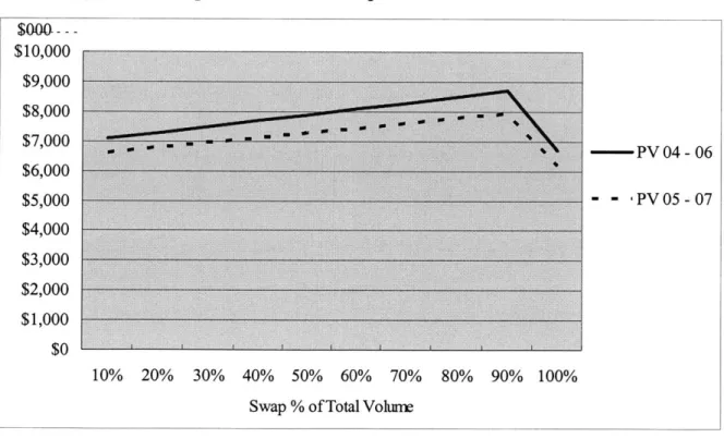
Figure 9. Total present Cost and swap ratio of total volume ... 66
Sensitivity analysis: Sensitivity analysis: Sensitivity Sensitivity Sensitivity Sensitivity Sensitivity Sensitivity Sensitivity Sensitivity Sensitivity Sensitivity Sensitivity Sensitivity Sensitivity Sensitivity Sensitivity Sensitivity analysis: analysis: analysis: analysis: analysis: analysis: analysis: analysis: analysis: analysis: analysis: analysis: analysis: analysis: analysis: analysis: present value and switching cost to swap...79
option value and switching cost to swap ... 80
present value and switching cost to repair...81
option value and switching cost to repair...82
present value and volatility of swap model...83
option value and volatility of swap model ... 84
present value and volatility of repair model...85
option value and volatility of repair model ... 85
present value and customer relationship ... 88
option value and customer relationship...88
present value and repair overhead cost...90
option value and repair overhead cost ... 90
present value and repair unit cost ... 91
option value and repair unit cost ... 91
present value and product unit cost ... 92
option value and product unit cost ... 93
present value and return volume ... 94
option value and return volume...94 Figure 10. Figure 11. Figure 12. Figure 13. Figure 14. Figure 15. Figure 16. Figure 17. Figure 18. Figure 19. Figure 20. Figure 21. Figure 22. Figure 23. Figure 24. Figure 25. Figure 26. Figure 27.
List of Tables
Table 1. Decisions around reverse logistics system review ... 22
Table 2. Example of decisions around reverse logistics system review...23
Table 3. Total cost for repair everything model...26
Table 4: Total cost for the swap everything model...29
Table 5: Value of call option... 39
Table 6. Overage and underage costs ... 51
Table 7. News Vendor Approach for Repair Everything Model...54
Table 8. DCF analysis for repair everything model ... 60
Table 9. News vendor approach for swap everything model ... 62
Table 10. DCF analysis for swap everything model...64
Table 11. Swap ratio and present value ... 66
Table 12. Sensitivity analysis for repair everything model...67
Table 13. Sensitivity analysis for swap everything model ... 68
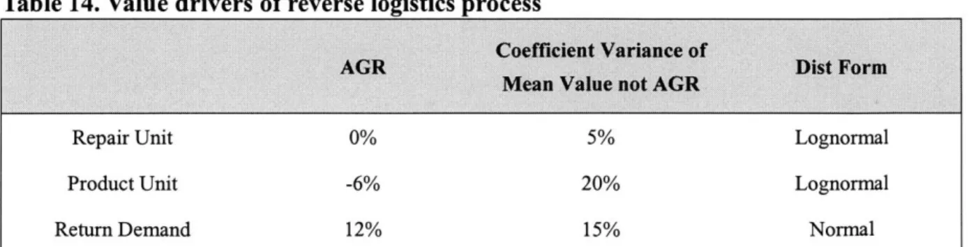
Table 14. Value drivers of reverse logistics process...70
Table 15. Real options analysis for repair model with switching option to swap ... 72
Table 16. Real options analysis for swap model with switching option to repair...76
Table 17. Summary of the result of real options analysis...77
Table 18. Summary of the sensitivity analysis around the optimal model...95
1. INTRODUCTION
In this chapter, the key research questions and methodology are described. Additionally, the importance of real options in logistics is discussed and a general roadmap of the thesis is provided.
1.1. Background
This thesis addresses the problem of a reverse logistics process for the circuit board business. The objective is to minimize the cost of reverse logistics operations over the next few years. The specific question we ask is, "Which method is the cheapest when you process return products - repairing, swapping, or switching between the two operational models?"
We examine the reverse logistics process of a technology company (called company X hereafter due to confidentiality). The current operational model is to repair return products as much as possible (some return products cannot be repaired and need to be replaced with new products). In recent years, the circuit board market has been growing rapidly, so the new product cost is approaching the level of the repair cost. This is why company X is considering an alternative operational model called the swap model. Under the swap model, all return products are scrapped and new products are shipped to the customer. The issues here are uncertainty in product cost, repair cost, and return volume. Because of the high fluctuation of the product cost as shown in Figure 1, the product cost can become more or less expensive than the repair cost. This makes it difficult to plan an optimal model for the next few years.
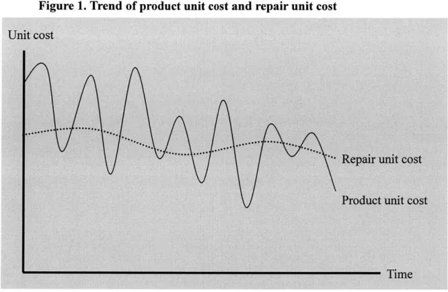
Figure 1. Trend of product unit cost and repair unit cost
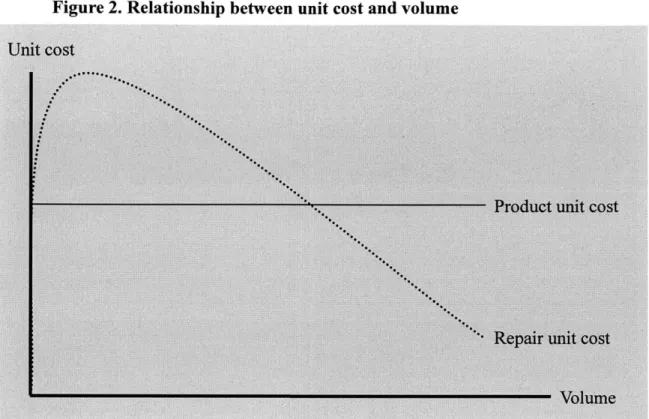
What makes the planning more complicated is that the repair unit cost is affected by the return volume, which also shows a long term growth trend with volatility. As Figure 2 shows, there are economies of scale in the repair unit cost when the volume increases. This is because the fixed cost of repair operations can be smaller at a per unit level as the volume increases. On the other hand, the new product unit cost is not sensitive to the volume changes, for the new product unit cost does not incur any fixed cost. As Figure 3 shows, due to these economies of scale, the total cost of the repair model can be cheaper than the total cost of the new product swap model. So even though the product unit cost is declining, the increasing trend of the return volume may keep the current repair operation cheaper than the alternative new product swap operation.
Figure 2. Relationship between unit cost and volume
In such an uncertain situation, the switching option between the repair and swap models can become valuable. For example, the new product swap operation can be used as the basic operational model as the product cost is declining in the long run. Meanwhile, the repair operation can be kept as an option to exercise when the product cost becomes higher than the repair cost in the short term fluctuation. In a sense, the repair option for a high value product (some circuit boards have relatively high value) is like auto insurance for an expensive car. When you cannot replace the car with a new one at a reasonable price, you need to use your insurance money to repair it.
However, if the price of the car drops and the price of insurance remains relatively high, you may want to get rid of the insurance. Why spend $200 insurance per month for a $2000 car? If the new product cost drops below the repair cost, why keep expensive repair operations as insurance? Conversely, if the product cost picks up well above the repair cost, it is better to keep the repair option. Keeping the repair option fosters flexibility as a hedging mechanism for the uncertainty in the product cost. It should be noted, however, that keeping the option not only provides value but also costs.
1.2. Research Questions and Motivation
The main research questions to be addressed in this thesis are:
* What is the optimal model for the reverse logistics process, taking into consideration the trend and volatility of the repair cost, the new product cost, and the volume? * What are the cost savings and risks associated with different models over the next few
How much should be paid to obtain the option?
* How robust is the optimal model when the variables deviate from the forecasts and assumptions?
Because of the simultaneously changing variables over multi-periods, the optimization approach, which simply chooses the lowest cost model using fixed values for variables, is not appropriate to answer the questions above. Sensitivity analysis may help, but it does not measure the impact of the variables that change simultaneously over the time horizon. Discounted cash flow analysis takes into account the changing variables over time but does not provide the degree of risks or the value of the option. Discounted cash flow analysis with Monte Carlo simulation can show the degree of risks by simulating the variables that follow their probability distributions. However, it cannot provide the value of option. Therefore, real options analysis is used to identify an optimal model with a value of option. The fundamental difference between the simulation concept and the option concept is contingent strategy. Simulation says, "If variables A, B, and C change, X happens." But it does not incorporate chess-like thinking, "If X happens, do Y." On the other hand, the options concept is the contingent strategy, and this is why it makes a significant difference in uncertain situations.
There have been many instances of real options application to capital intensive projects, such as an electric power plant, a gold mine, an oil field, real estate development, and pharmaceutical R&D. On the other hand, real options have rarely been applied to logistics systems or processes (real options have been used to analyze supply chain management, especially supply contract). In the future, real options will become increasingly important in analyzing logistics systems because they are becoming more
Because of this uncertainty, it is often the case that everyone has subjective prospects and the mentality "there is no right answer" prevails. This is why a warehouse manager mentioned that all logistics consultants gave different solutions for the optimal
warehousing location. According to Amram and Kulatilaka [1998], "In volatile markets, where prices and demand are always in flux, it is hard to predict how a particular
investment will ultimately influence a company's value. Senior executives spend a lot of time structuring their decisions, tracing possible implications, assigning probabilities, and assessing risk. Rarely, though, does everyone agree about how an investment will play out." Real options would help resolve the difference in personal views by bringing in financial options theory.
There are many potential logistics problems that real options is good at solving. For example, a shipper that normally uses air freight may want to consider obtaining the option of using sea freight in case air freight cost goes up dramatically. This was a problem faced by shippers a few years ago when the air freight cost increased dramatically because of the security surcharge introduced after September 1 1th and the fuel surcharge increased due to the Iraqi war. In fact, many shippers shifted to sea freight. Another example is that Asia is becoming a world factory, and there is a high concentration of export freights at a few hubs such as Hong Kong, Shanghai, and Singapore. The costs of freight from these hubs are becoming higher, and the capacity is getting tight, so it may be wise to obtain an option to use different logistics hubs to manage freight cost and capacity. Real options helps quantify the value of such options and clarify how much should be paid to keep the option. As real options are becoming important to solve logistics problems, the
1.3. Roadmap of Thesis
The reminder of this thesis is organized as follows. In chapter 2, the current reverse logistics practice of company X is described and alternative models including switching options are introduced. In chapter 3, the real options literature is reviewed, the concept is introduced, and the steps for conducting real options analysis are described. In chapter 4, to determine the inventory policy applicable to different reverse logistics models, the news vendor approach is used and modified to consider the multi-product lines that company X currently handles. In chapter 5, discounted cash flow analysis, Monte Carlo simulation, and real options analysis are performed to evaluate the cost saving of different models and the value of the switching option. (See Figure 4 for the connections of different analyses.) The sensitivity analysis for the optimal model is also conducted at the end of chapter 5. In chapter 6, the result is evaluated in light of the implementation costs as well as key
sensitivities. Finally, areas of further research are discussed.
2. COMPANY BACKGROUND
This chapter clarifies the company objective to minimize the cost of the reverse logistics process. Additionally, the current model for the reverse logistics process and the
alternative models including the switching option are discussed. Most of the content of this chapter is based on the internal documentation of and the interview with company X.
2.1. Company Objective
In this section, the size and cost of the reverse logistics of company X, as well as the reverse logistics organization and processes are mentioned. At the end of the section, the
cost issue is emphasized as a company objective.
2.1.1. Introduction
Company X holds 10% of the circuit board market worldwide. Over the past year, approximately 3% of the circuit boards sold by company X have been returned. This 3% includes products returned as defective (2%) as well as customer stock rotations (1%). Most of the returned circuit boards come from two major customer segments: large
electronics manufactures and wholesale distributors who resell circuit boards to small individual customers. Half of the volume is from large electronics manufacturers and half comes from wholesalers. Recently the volume from wholesalers has been growing
Operational costs for the reverse logistics process can be divided into repair costs and swap exchange costs. Over the past year, more than $20 million was spent for repairing circuit boards. The cost associated with the swap has grown significantly over the past few years and has now reached $10 million. These figures exclude transportation costs, swap product costs, and inventory holding costs. These costs are not easy to capture because some of them are tracked at the business unit level, while other costs are tracked at the corporate level. There has been pressure to reduce the reverse logistics costs because the circuit board business has become less and less profitable.
2.1.2. Organization and Network
Company X's reverse logistics group serves electronics manufactures and wholesalers by providing warranty repair, product replacement, failure analysis, and credit compensation. The mission of this group is to protect customer loyalty and assist product improvement.
The primary regional headquarters of the reverse logistic group are in the U.S. for North America, in Ireland for Europe, and in Malaysia for Asia. Repair capability is mostly outsourced, with 80% of American operations handled by a contract manufacturer in Mexico and 100% of European operations handled by a contract manufacturer in Hungary. Repair operations in Japan, China, and India are also outsourced.
In-house repair capability is in the U.S., where most sophisticated operation lies, and in Malaysia, where most of the repair volume in Asia is handled. In-house capability has taken an important role in transferring knowledge and skills to the repair outsourcing company. Repair operations at company X have followed the outsourcing trend in its
circuit board manufacturing. Most of the effort in recent years has been spent for knowledge transfer to and start up of repair outsourcing, so the forecast for outsourcing repair costs remains uncertain. This is one of the risky factors involved in planning an optimal operational model in the next few years.
Exchange depots for wholesale customers are spread over the U.S., China, Russia, Asia, India, Europe, and Latin America (see Figure 5). All depots are run by third party logistics providers. Unlike the repair operations, the logistics costs paid to the third party logistics providers are relatively stable.
Figure 5. Reverse Logistics Worldwide Network
Europe... Ireland Americas KY pan FL China Mexico Asia BrazilMalaysia South Africa 9 Australia
+
Regional Headquarter iW Outsource Repair Location2.1.3. Return Profile
Returns due to either stock rotations or product failure during the assembly process are termed RMA (return material authorization) returns. Defective RMAs are issued only if items are likely to be repaired. They are restocked to inventory and eventually swapped with return products. Stock rotation RMAs can be put back into inventory.
Circuit boards that failed when used by the end users are called DRA returns (direct return authorization). All returned DRAs are considered broken and are repaired and sent back directly to the customer. DRAs are expected to be repaired within 10 days and RMAs within 30 days. The optimal backlog has tended to be around 4 to 5 days of work to provide good batching. Because RMA repairs are less time sensitive, they are often used to smooth out the repair volume. Volume fluctuations can vary widely from week to week. For example, during an average one week period, the standard deviation of total receipts is 24%. There are also quarter to quarter fluctuations due to seasonality. These standard deviations are less pronounced at 6%, and the annualized standard deviation is 15%.
2.1.4. Repair, Swap, and Scrap Processes
All defective products are first swapped with the products (new or repaired) in inventory. Then the returned products get screened to see whether they are repairable. If they are, they are sent to a repair outsource location, and if not, they are sent to a scrap site. If scrapped, they need to be replaced with new products sent from the manufacturing site of company X at the beginning of each product lifecycle, which is three years. Therefore, this is a single period inventory replenishment, which will be discussed in Chapter 4:
Inventory Policy. While RMA and DRA are handled similarly across customer segments, processes around swap, repair, and scrap are handled differently, depending on whether the customer is a large manufacturer or a wholesaler.
Large manufacturers are served at a depot next to the manufacturing site. The depot provides special service and handles large volumes. Meanwhile, all wholesalers are handled by a regional depot. The volume split between electronics manufacturers and depot is about half and half, as the volume handled by wholesalers has increased
dramatically in recent years. This thesis focuses on depot operations in the U.S. as a pilot project. If this project proves to be successful, the model should be rolled out for both wholesalers and electronics manufacturers worldwide. The volume handled by the U.S. depot operation is only 10% of worldwide volume, so the impact can be much more than that of the U.S. depot operation. In any case, it should be noted that only the U.S. depot operation is discussed in the following.
When a defective product is returned to a depot from a wholesaler, it is screened to verify the claimed defection. Currently minor screening at the depot is not implemented for every product, but it is going to start by the end of 2004 to reduce the volume shipped to the repair outsourcing company. Therefore, in this thesis, it is assumed that there is already a minor screening for all products at a depot site, and the screening reduces the current volume by 40%. If there is no defection found through minor screening, the board is sent back to the customer. If defection is confirmed, it is sent from the depot in the U.S. to the repair outsourcing company in Mexico.
"repair board" and if it cannot be fixed, it is a "scrap board." To determine the cause of a failure, a board may need to pass through debug and repair loops multiple times and undergo subsequent testing. Therefore, the average board goes through some activities more than once, and hence the process can become quite complicated.
While the return product is sent to Mexico, a swap board in the inventory at the depot in the U.S. is sent to customers. This shortens the wait time but is costly to operate from an inventory holding cost perspective. If boards are repaired and placed into inventory, they are subject to having to be re-upgraded if a new mandatory revision is released. Also, inventory must be tracked not only by part number, but also by revision level to ensure no improper down-revision boards are sent to customers. Meanwhile, old leftover boards can hardly be upgraded and replenished to the inventory when stock out occurs.
New swap boards sent from the manufacturing site of company X are used to help replace boards that could not be fixed (scrap) and therefore mitigate credit costs. Credit would otherwise have to be paid to customers when a board under warranty cannot be replaced. Currently, approximately 10% of the return volume is swapped with new products and scrapped. Company X is considering increasing the percentage as the cost of new product is declining compared to repair costs. However, one of the problems with the new
product swap process is that it usually ends up leaving excess inventory or stock outs.
2.1.5. Cost Issue
The circuit board business can no longer afford what they have been spending on warranty returns. Competition in recent years has become fierce among the major circuit board
manufacturers, and every penny is scrutinized as circuit board manufacturers struggle to break even. Since most of the product cost is materials-related and viewed to be fairly
fixed, the remaining costs, such as warranty-related costs are increasingly being examined for any possible savings opportunities.
Additionally, recent industry benchmarking research suggests that company X has spent more money on its reverse logistics, while it provides a lesser degree of customer
satisfaction than its competitors. Furthermore, scalability to meet the growing needs of the business is poor, and the gap is going to increase with expected growth in volume, if the reverse logistics process remains the same.
A reverse logistics manager at Company X says, "The only boundary conditions are that the solution cannot negatively impact our current customer terms and conditions (such as service level, etc.), and the savings must be real savings to the company, not saving money for one business unit at the expense of another or 'funny money' type allocation games, which move spending from our books to another's." Clearly, the objective function is to minimize cost subject to the given service level and demand volume.
2.2. Problem Definition
This discusses different approaches to streamline the reverse logistics system. The reverse logistics process is identified as the focus of cost improvement. For the process, both the current and alternative models, including a switching option are discussed.
2.2.1. Approaches
In order to reduce reverse logistics costs, basic questions need to be answered as follows. The answers to the question should vary for each customer segment.
" Who handles reverse logistics operations? Should the operation be kept in-house or outsourced?
* What kind of operational model should be taken? Which is cost optimal with
moderate risks, the repair model or the swap model? Is the switching option valuable? * How long should the lead time be?
* How many repair centers and depots should be deployed?
* Should operations be located in each region, i.e. the U.S., Europe, and Asia? Or should it be centralized at one region?
Below is the example of decision sets for the reveres logistics case.
Table 1. Decisions around reverse
Small but highly profitable In-house New product swap everything
10 days 3 depots Global
Mid Outsource 2 depots and U.S., Europe,
Hybrid 15 days 1 repair
customers Firm X Asia
center Large but less profitable Outsource Firm Y Repair everything 20 days 1 repair center + 1 depot ________________________ I ________________________ I _________________________ L ________________________ .1 Combination Examples I
Table 2. Examnile of decisions around reverse I
Outsource 3PL New product
swap everything 10 days 3 depots Regional
Outsource 1 repair
Large PC Rpi
Contract epair 15 days center, 1 Global
Manufacturer eeyhn
Manufacturing depot
In this example, wholesalers are supported through depot swap operations by third party logistics providers. To maintain relatively short lead times, company X uses a new
product swap process in which the depots are scattered to each region. On the other hand, large electronics manufacturers can allow a longer lead time, so company X chooses repair operation, which is handled by outsourcing repair companies that have flexibility and economies of scale. To further leverage economies of scale, company X has globally centralized repair and depot operations at more cost efficient locations, such as China.
In the past five years, company X has made decisions about most of these questions. They have differentiated the service offerings based on the customer segment. They have expanded externalized repair operations significantly by outsourcing 100% of the operation in Europe and 80% of the operation in the U.S. The number of depot locations has been trimmed and streamlined. Company X has determined that regional operations across the
U.S., Europe, and Asia make better sense to balance operating costs, labor costs, logistics
costs, lead time requirements, and operational and political risks.
Thus, company X is now turning its attention to the operations process. Cost drivers of operations such as repair costs, product costs, and volumes fluctuate over time, making it
month-to-month volume fluctuation, but it shows a long-term growth trend. Repair cost per circuit board can fluctuate, depending on the volume fluctuation and must be reviewed every quarter. The product price, which affects new product swap cost, changes at every product release, but shows a declining trend in the long run. Company X needs to review the operations process models taking these uncertainties into consideration.
2.2.2. Current Model: Repair Everything Model
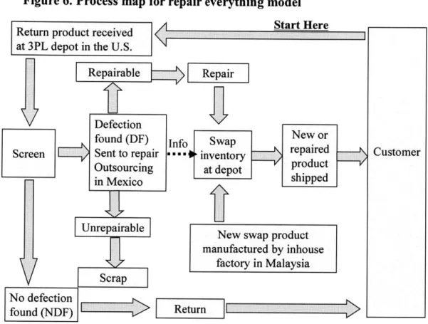
As it has been implied above, the reverse logistics process review is about how much split should be made between new product swap and repair. The current U.S. depot operation is the so-called repair everything model. Under the repair everything model, 90% of return volume is repaired, and 10% of return volume is scrapped and swapped with new products. The reason why 100% of return volume is not repaired is that 10% of total return volume is too defective to repair: they need to be scrapped and swapped with new circuit boards. The repair everything process is mentioned also in 2.1.4: Repair, Swap, and Scrap Processes. But because this is one of the key concepts in this thesis, the process is explained here. As the following process map shows, the return process of the repair everything model starts when a customer returns a circuit board to company X's depot, a division run by 3PL in the U.S. Once the board is received at the depot, it is screened to confirm whether it is actually defective or not. If no defect is found, the board is returned to the customer. If a defect is found, it is communicated to the shipping operation and a new or repaired board is sent to the customer. Meanwhile, the defective board is sent to an outsourcing company in Mexico to be repaired. If the board is deemed unrepairable through the repair process, it is scrapped. If the board is repaired, it is sent back to inventory in the depot to replace another defective product and be shipped to customers.
Because about 10% of total return volume is deemed unrepairable, new products, which account for 10% of forecasted total volume, are ordered from company X's manufacturing site in Malaysia at the beginning of the release of each product line.
Figure 6. Process map for repair everything model
Start Here
Return product received at 3PL depot in the U.S.
Repairable Repair
Defection
found (DF) Info Swap Ne C
Screen Sent to repair --- inventory repaired Customer Outsourcing at depotpd
in Mexico shipped
Unrepairable New swap product
manufactured by inhouse factory in Malaysia Scrap
No defection
found (NDF) Return
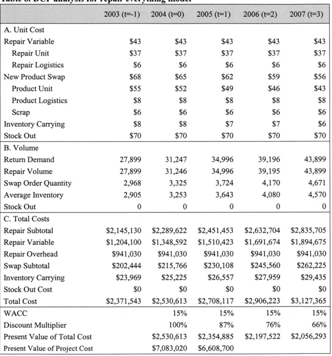
Total costs for the current repair everything model can be calculated as in the following table and the cost components are explained below. Note that all data is actual data in the year of 2003.
Table 3. Total cost for repair everything model
Repair Variable $43 27,899 $1,204,100
Repair Unit $37
Repair Logistics $6
Repair Overhead $941,030
New Product Swap Variable $68 2,968 $202,444
Product Unit $55 Product Logistics $8 Scrap $6 Inventory Carrying $8 2,905 $23,969 Total Cost $2,371,543 A. Unit cost
The repair variable cost is the sum of the following cost items.
* The repair unit cost: this is charged by repair outsourcing company.
" The repair logistics cost includes freight and handling between depot and repair
outsourcing company.
The repair overhead cost includes the cost of information systems infrastructure for the reverse logistics process and the cost of staff to manage the repair outsourcing company. The overhead cost was approximated in the following manner: the overhead cost at the U.S. depot was considered equal to the worldwide overhead cost times 10%. The 10% came from the volume at the U.S. depot divided by worldwide volume.
New product swap variable cost is the sum of the following costs items.
* The product unit cost is the amount charged at company X's factory in Malaysia.
site to the depot charged by the third party logistics provider.
* The scrap unit cost includes the logistics cost to the scrap site and the actual scrap process cost.
Inventory carrying cost is defined as the product unit cost times the weighted average cost of capital. Weighted average cost of capital of company X is 15%, which is relatively higher than other industries because of the risky nature of the technology industry.
B. Volume
Repair volume is calculated as follows:
Repair volume = (total returned volume -new product swap volume) x 10/9
Because new product swap volume is first determined at the beginning of the release of each product, new product volume should be consumed first to replace return volume. After all new product volume is swapped, the repaired volume needs to replace the rest of the return volume which is the total return volume minus the new product swap volume.
The reason why the difference is multiplied by 10/9 is that 10% of the repair volume does not get fixed as mentioned before, so the volume that goes through the repair process
(including repairable and unrepairable items) must be inflated by this percentage.
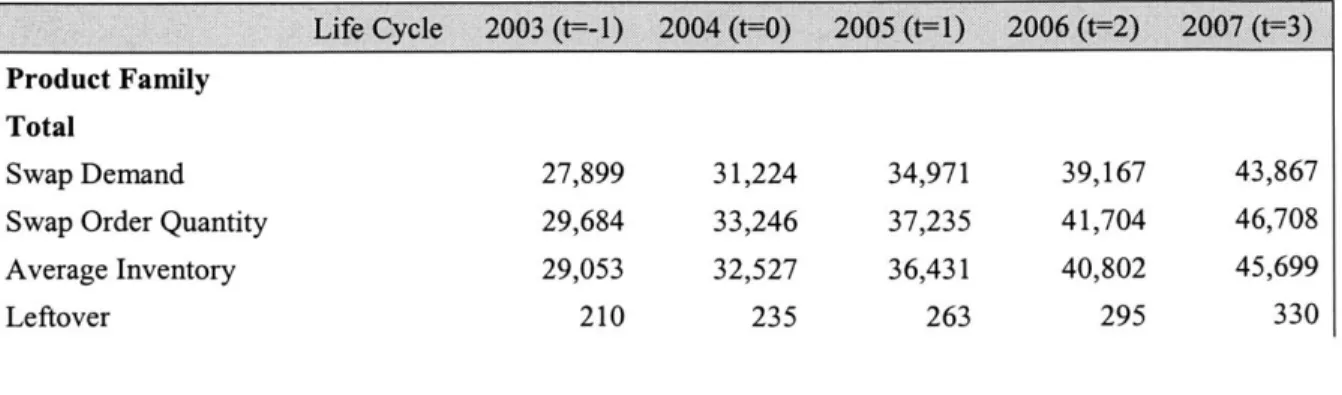
New product swap volume and inventory carrying volume is determined by the news vendor approach, which is discussed in Chapter 4: Inventory Policy. It should be noted that all inventory for new product swap volume is purchased at the beginning of the year for the next three years of product life cycle. Therefore, this is a single period inventory problem or so-called news vendor problem.
2.2.3. Alternative Model: Swap Everything Model
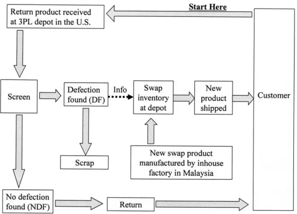
While the repair everything model strives to repair as much as possible, which is usually 90% of total volume, the swap everything model replaces all return products with new products and all return products are scrapped. Because there is no repair operation, stock out can occur.
As the process map below shows, the return process of the swap everything model starts when a customer returns a circuit board to company X's depot. Once the board is received at the depot, it is screened to confirm whether it is actually defective or not. If no defects are found, the board is sent back to the customer. If a defect is found, it is communicated to the shipping operation and the new board is sent to the customer.
Meanwhile, the defective board is sent to a scrap site and gets scrapped. The inventory is replenished by only new products (not repaired products) sent from company X's
manufacturing site in Malaysia at the beginning of the release of each product line.
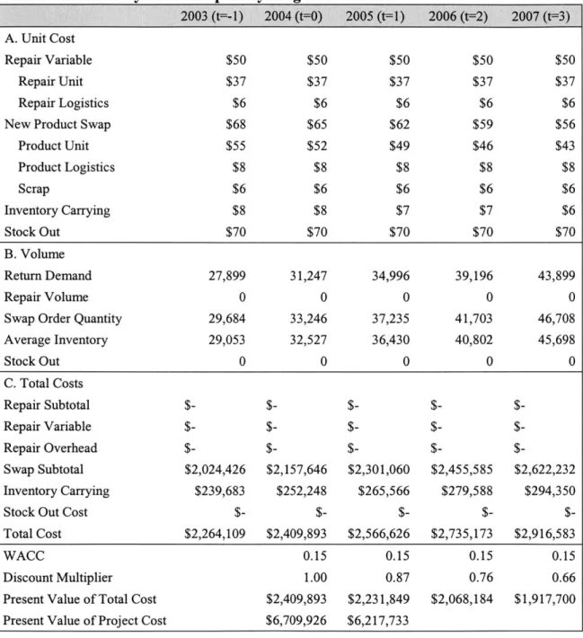
Total costs for the swap everything model can be calculated as in the Table 4. (It is assumed that the alternative model had been taken in 2003.) The cost components are the same as in the repair everything model and they are already explained above.
for the swap everything model
Return product received at 3PL depot in the U.S.
Defection Info Swa Screen found (DF) *---* invent at de y N Scrap manu fac No defection found(NDF) Return p New ory product )ot shipped -w swap product factured by inhouse tory in Malaysia
Table 4: Total cost for the swan everv
Repair Variable $43 0 $0
Repair Unit $37
Repair Logistics $6
Repair Overhead $0
New Product Swap Variable $68 29,684 $2,024,440
Product Unit $55 Product Logistics $8 Scrap $6 Inventory Carrying $8 29,053 $239,685 Total Cost $2,264,125
11
Start Here Customer Figure 7. Process mapAs the total cost tables of the two models show, the swap everything model is slightly more cost effective, that is, about $0.1 million less than the current repair everything model. However, in the reverse logistics process review that examines the optimal model in the next three to four years, this information is not sufficient because the costs and volume change over the time horizon. Therefore, discounted cash flow analysis is more
appropriate to evaluate the cost efficiency of the two models. The discounted cash flow analysis for the two models is discussed in Section 5.1: Discounted Cash Flow Analysis.
2.2.4. Switching Option
Another alternative is to keep the swap option with the basis of the repair model. Company X can maintain the repair model as a normal operation, and when the swap model becomes more cost effective than the repair model, company X should exercise the
switching option to new product swap. This situation is highly likely because product cost has shown a long term decline with short term fluctuations in response to volatile circuit board volume.
The opposite model, which is the repair model with a switching option to repair, is also possible. Intuitively, this fits the trend of product cost above. In the long run, the
product cost is declining, so the new product swap model should be used as the basis, while in the short term the increase in product cost makes the switching option to repair more valuable. Additionally, when there is no more new product to swap, the switching option to repair would prevent a stock out situation.
The switching option is a good alternative to consider rather than just examining the repair everything model or the swap everything model. Switching options in real options analysis can help choose which model is optimal. Real options analysis can not only value the switching option quantitatively but also shows total present value of each model with risk measures if used with the discounted cash flow model. In the next chapter, the recent literature on real options is introduced, examples of switching options are explained, and steps for real options analysis is discussed.
3. METHODOLOGY
In this chapter, the steps to conduct real options analysis are discussed. Specifically, the binomial model and Monte Carlo simulations are explained. Additionally, the literature review on real options and the classifications and approaches within real options analysis are introduced.
3.1. Literature Review
After the literature on real options is reviewed, the literature specifically on logistics problems is introduced. Then, the frameworks and examples of switching options are discussed.
3.1.1. Real Options
Myers [1977] first used the term "real options" when he applied financial options theory to value real assets projects with flexibility. While interest in this subject was limited to academia in the 1980's, interest has increased significantly in the 1990's. In the past decade, not only has the theoretical framework been strengthened but also the application range has been expanded. As a result, practitioners such as management consultants and business analysts have begun to apply the tool for business valuation, project investment,
and corporate strategy. Real options have been developed and applied to many areas.
option, switching option, and compound options) have been discussed as follows. The value of the timing option to wait for better information was identified quantitatively as most investment decisions are irreversible (Dixit and Pyndick, 1994). Additionally, the
growth option of investors for a venture business was explained by real options (Sahlman, 1997). The switching option for closing and reopening a gold mine was also evaluated by real options (Moel and Tufano, 1998 and Luenberger 1998). Compound options were discussed in many cases such as the oil field lease, Ford's investment in fuel cell
technology, and R&D in the pharmaceutical industry (Paddock, Siegel, and Smith 1998, Oueslati, 1999, and Schwartz and Moon, 1999). Furthermore, the impact of competition on compound options was examined (Triegrogis, 1996).
Aside from the discussion of these types within real options, various decision-making frameworks related to real options have been developed. In a strict sense, real options is derived from financial options theory, so only the Black-Scholes model or the binomial model should be used. However, a more qualitative approach has been developed (Boer, 2002). For example, decision analysis instead of financial options models was applied to approximate the value of option (Faulkner, 1996). They hybrid method was also used to analyze project risks with real options analysis and market risks with decision tree analysis (Neely and de Neufville, 2001). Moreover, simulation was applied to calculate multiple interacting options on a harbor project (Juan et al., 2002). Finally, the advantages and disadvantages of these different approaches were discussed (Borison, 2003).
Besides the academic discussions above, the practical application process of real options as a consultant and a business analyst have been introduced (Rogers, 2002 and Brach, 2003). Specifically, an underlying asset was defined as the present value of a project and a Monte
and Antikarov, 2001). Furthermore, a real options software program called Crystal Ball was introduced (Mun, 2003).
3.1.2. Real Options Application to Logistics Problems
The real options application has also expanded to the area of logistics and supply chain management. For example, Hewlett Packard has tried to apply real options to their business operations since the 1990's. As a result, HP has developed a postponement strategy to customize inkjet printers at assembly sites closer to the demand locations as demand uncertainty unfolded (Billington, C., Johnson, B., and Triantis, A., 2002). From an academic perspective, Van Hoek [2001] mentions postponement strategy to retailer order to cope with the seasonal cycle.
In addition to postponement, real options applications are concentrated around supply chain management, specifically supplier relationships. Tan [2001] valued a contingent capacity agreement to meet unexpectedly high demand. Another example is that Pochard [2003] applied real options analysis to value dual sourcing strategies. With real options, sourcing decisions can be adapted to changes in risk parameters. Related to dual sourcing, Sheffi [2001] discussed that redundancy can respond better to supply chain disruptions. Martha and Subbakrishna [2001] also recommended that firms add redundancies in supply
resources, transportation modes, inventory stocks, and process. They also discussed that flexibility such as switching option and postponement can replace redundancies.
3.1.3. Switching Option
According to Brach [2003], "switching option captures the managerial flexibility to alter the modus operandi of any given business. This includes exchanging input or output parameters, volume, processes, and global locations. The value drivers of the switching
option include the costs saved and additional cash flows generated by having the ability to respond to future uncertainties and change a cost-driving operational parameter."
There are many examples of switching options. GM's plants have the flexibility to switch output from one car model to a different one to respond to demand change in car models. Enron utilized the switching option between different fuel sources to take advantage of cost
fluctuations of the fuel sources.
Tufano and Moel [2000] use an example of gold mine operations to illustrate how real options analysis can value the switching options. Let us assume that the average
exploitation cost is $300 per ounce and that the international price of gold is currently $350 per ounce. Intuitively, it seems that if the international price falls below $300, the mine field should be closed. However, the following factors make this problem more
complicated.
* Fixed costs for closing and restart, such as paying retirement benefits, retraining, and redeploying equipment are high and overall costs may actually increase if the mine is shut down and restarted frequently without keeping fixed assets alive.
" The price of gold fluctuates and is uncertain. Soon after closing the mine, the price may rise above $300 per ounce. Then, the cost to restart would incur the
Therefore, maintaining the flexibility to stop and restart would increase the value of mine operations. The value of the flexibility, the switching option, primarily depends on the volatility of fixed costs, price, and exploitation cost.
Another example would be a lay-off policy with partial compensation. By spending partial wages during the lay-off period, an employer can avoid incurring hiring and training costs when business picks up again. But this option should be used only when the value of retaining employees outweighs the cost of the partial wage.
In the technology industry, alternative processes and capacities can provide important flexibility. According to Billington, Johnson, and Triantis [2002], "these processes may differ in terms of fixed cost, variable cost, throughput, or lead time. For instance, a high-volume process with high fixed costs but low variable costs can be used as base capacity to satisfy a large component of expected demand. If demand exceeds this base level, additional capacity with lower fixed but higher variable costs can then be brought on to manage such short-term fluctuations."
In this thesis, real option analysis will show the value of the option to switch between repair and swap models. The option value will be the maximum amount that company X should spend to keep the switching option. While it is reasonable to keep options open just in case, keeping options open comes at a cost. What makes the theory of real options
useful is that it quantifies the value of options so that you know how much you should spend to obtain the option. The framework of real options is explained in the following section.
3.2. Real Options Analysis
This section explains the mechanics of real options analysis. Specifically, the binomial model and Monte Carlo simulations are explained. Then the four steps to conduct the
analysis are developed. Different classifications and approaches within real options are also introduced.
3.2.1. Introduction
Real options is like call and put in financial options. The call option is the right to buy stock if the stock price becomes higher than the predetermined price under the call option. Basically this is "riding gains" when outcome becomes favorable. The put option
purchases the right to sell a stock when the stock price becomes lower than the
predetermined selling price under the put option. This is an example of "cutting losses" when outcome becomes unfavorable.
In the case of the swap model with a switching option to repair, the call option is like exercising the repair option when the product cost rises above the repair cost. Similarly, the put option is like switching back to the swap model when the product cost falls back below the repair cost. The term "real options" means options on real assets, such as logistics processes, facilities, locations, etc., instead of financial options on stocks and bonds.
positive and a negative direction. The following is an example of how options make it possible to capture most of the upside swing while protecting against most of the downside swing and hence produce better expected profit without options.
Let us assume that a $200 stock can increase to $300 or decrease to $100 with a probability of 50% in one month. If you purchase the $200 stock now to sell it in one month, there is a 50% risk that you could lose $100, while you could also make $100 with the same probability. Therefore, the expected profit of the investment is calculated as follows.
$0 = 50 % x $100 + 50% x (- $100)
Meanwhile, if you pay the option price of $20 and obtain a call option with the
predetermined exercise price of $200 in one month, you will be able to buy the stock with the $200 when the actual stock price goes up to $300 in one month. By taking advantage of the upside opportunity, you can make a profit of $80 ($100 (capital gain) -$20 (option price)). Even if the stock price drops to $100, you are not obliged to purchase and just
lose the small option price. Consequently, the expected profit becomes as follows.
$30 = 50 % x $80 + 50% x (-$20)
Table 5 shows that the value of the option is $30, the difference between the expected profit with and without option.
With Option $20 $80 $30
3.2.2. Classifications and Approaches of Real Options
Before discussing the classification and approaches of real options, other decision-making frameworks closely related to real options should be discussed to emphasize the usefulness of real options under uncertainty. According to Amram and Kulatilaka [2001], other frameworks have the shortcomings that real options can overcome in the following ways.
* Scenario-based discounted cash flow method
The traditional discounted cash flow (DCF) model does not consider uncertainty, as it assumes single values for each variable. Meanwhile, managers can use DCF even under uncertain situations if DCF is performed in different scenarios. However, the problem of scenario-based DCF is that the probability of each scenario is set
subjectively. Additionally, there is no chess-like thinking, i.e. "if A happens, do B." Scenario-based DCF simply says, "If A happens, the result would be C." So it does not consider contingent strategies under uncertainty.
* Decision analysis (or decision tree analysis)
This portrays the decision framework with a decision tree, which incorporates
chess-like thinking i.e. "if A happens, do B." This is easy to understand, but in decision
quantification because of subjectivity, the analysis becomes qualitative and can be useful for creating strategy. However, it fails to become an investment decision
framework.
* Simulation
Simulation provides thousands of values for each variable, following given mean value and probability distributions of the variable. As a result, mean value and probability distributions of the outcome can be captured, and hence, risk can be assessed.
However, simulation does not provide contingent strategies.
Real options analysis incorporates contingent strategies and uses objective probability under no-arbitrage assumption, the first principle of financial theory. Let us assume that IBM is trading at $100 in New York, GBP 60 in London, and JPY 11,000 in Tokyo. As a result of arbitrage behavior of investors taking advantage of the different prices in the three markets, all the prices in these markets converge into one and there is a no-arbitrage
opportunity in the financial markets. This assumption of the financial theory is applied to real options and this is why returns of all projects converge into the risk free rate (this is typically the short term interest rate of the U.S. government bond). Based on the risk free rate and the volatility of projects, the risk neutral probability of the up and down of an
underlying asset is determined. This is the ground that probabilities used in real options are objective. This will be explained in Section 3.2.3: Binomial Approach.
While the above is about decision frameworks related to real options, there are different classifications within real options. Amram and Kulatilaka [2001] divide real options into three categories: operational, investment, and contractual.
" Operational option
This option provides the flexibility to change inputs and outputs in response to changes in operational factors such as price, cost, and volume. The switching option is one of the operational options.
" Investment option
This is about whether to modify investment decisions during the project. A typical case is adjusting investment scale or timing, e.g. expand, contract, delay, or abandon a project. This classification has been the major area of real options application.
" Contractual option
An example of a contractual option would be that venture capitalists maintain special contractual clause to give the right to sell the asset of the venture business.
In addition to these classifications, there are different approaches within real options. Some of the most popular approaches are the Black Scholes model and the binomial model. According to Mun [2003], Black-Scholes is easy and quick to implement because all you need to do is to find the value of inputs to the Black-Scholes equation and calculate the equation. But it is difficult to explain because it requires knowledge of high level calculus. Additionally, there are many conditions required by the Black-Scholes model as follows:
* Options can be exercised only during the maturity period. This is called European options as opposed to American options that can be exercised anytime until the maturity period.
" There is no dividend paid by the underlying asset.
" Price and volatility of the underlying asset is market traded and observable. * Volatility of the underlying asset is fixed over time.
Because many real option cases do not meet the conditions required by the Black-Scholes model, the binomial model is normally used.
3.2.3. Binomial Model
Unlike Black-Scholes, the binomial model developed by Cox, Ross, and Rubenstein [1979] is easy to explain to business practitioners and is flexible enough to be applied to various cases in real options. The basic inputs of the binomial lattice and the description are as follows:
S: value of underlying assets, i.e. the present value of a real assets project ("S" has come from the capital letter of Stock price in financial options theory)
According to Copeland and Antikerov [2001], in many cases of real options, the underlying asset, a value of a project, is not publicly traded, unlike stocks and bonds defined as
underlying assets in financial options. For example, revenue or operational costs that can be an underlying asset of a real asset project are not publicly traded and their volatility is not observed in the market. Therefore, it is assumed that the present value of the project itself is the underlying assets. This assumption is called market asset disclaimer (MAD).
X: price of exercising option
capacity for the expansion option or the cost to switch one mode of operation to another for switching option.
g: volatility of the present value of the underlying asset
Volatility measures how hard it will be to predict the underlying asset's value into the future. According to Mun [2003], volatility is "the standard deviation of the lognormal growth of the present value of the cash flow at the current moment to the present value of cash flow at the next period. This can be expressed as follows.
Volatility = - Ln
PVt=
]PVt=0)j
It is important to note that only the numerator is simulated and the denominator is unchanged." The reason why volatility is the standard deviation, not of the present value itself but of the growth rate of the present value, is to measure the fluctuation around the growth trend and eliminate the trend factor and extract the risk factor.
He also adds that volatility can be "annualized value: multiplying it by the square root of stepping time breaks it down into the time-step's equivalent volatility. Stepping time is simply the timescale between steps. That is, if an option has ten steps in one year maturity, each stepping time becomes 0.1 years."
Volatility = - Ln =Ajlx
-- PVt=0) n
Where cY: standard deviation
T: maturity period or project period
Monte Carlo simulation provides the probability distribution and standard deviation of the lognormal growth rate. What it does in short is to show how the growth of present value of a project from time 0 to time 1 can change when inputs such as the repair cost, the product cost, and the volume change, following the given mean and standard deviation. The reason why the volatility is the standard deviation of the growth rate and not of the mean value of the present value of the project is to eliminate the trend factor and to measure the up and down factors around the trend. In other words, the volatility shows how unpredictable the present value of the project can be. Therefore, high volatility means high risk (both downside and upside).
rf: risk free rate or the rate of return on a riskless asset
This can be the interest rate of the U.S. short term government bond. Under no-arbitrage opportunity assumption, returns (growth rates) of all real asset projects converge into the risk free rate.
u: up factor
While returns of all real assets projects converge into the risk free rate, volatility remains specific to each project as risks remains different from project to project. The up factor is defined as the exponential function of the volatility multiplied by the square root of stepping time. The equation is as follows.
T
U = e " abeo
u = EXP(o*(SQRT(T/n)))
The stepping time is already explained in the section of volatility. As the value of the time step increases, the level of granularity, i.e. accuracy, increases and the result of the binomial model becomes similar to that of Black-Scholes (Copeland and Antikarov, 2001).
d: down factor
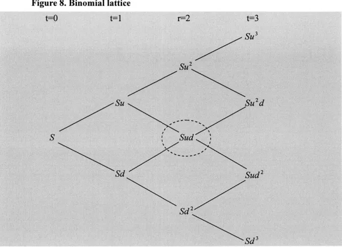
Down factor is simply the reciprocal of the up factor because of the assumption that the value of the underlying asset follows a multiplicative probability process (or geometric process). The multiplicative process is widely used, as opposed to the additive probability process (or arithmetic process), because the multiplicative process follows lognormal probability distribution that does not take negative values. Because of the multiplicative process, the binomial tree becomes recombining. "Recombining" means that the up and down trees meet at the node circled in Figure 8 below, and the multiplication of the two factors become 1 by the definition of the multiplicative process.
Figure 8. Binomial lattice
p: risk neutral probability for the up factor
Let S an expected present value of a project: let u up factor in one year and let d down factor in one year. The expected value of the project in one year is:
Su x p + Sd x (I - p)
Meanwhile the project grows with risk free rate because of the no-arbitrage assumption, so the expected value in one year is:
Therefore, the risk neutral probability is obtained as follows.
Su x p + Sd x
(1-
p)= S(i+ r)(1+
r - d)(u-d)
q: this equals to (1-p) and is the risk neutral probability for the down factor
p and q are mathematical intermediates to ensure risk neutrality of the binominal lattice.
With the inputs above, binomial lattice can be built and the lattice shows how the present value changes over time following the up and down factors. In Figure 8 in the previous page, in period 1, S (present value of project i.e. price of the project) becomes Su with risk neutral probability of p or Sd with risk neutral probability of u. In period 2, S becomes Su2 or Sud or Sd2. Because of the reciprocal magnitude (ud=1), lattices recombines at the circled area. In period 3, the range of the present value is between Sd3 and Su3
.
High volatility makes the value of the up and down factors large as shown in the equation in the up factor above. So the large value of the up and down factors makes the range of values between the upper and lower branches wider. On the other hand, the low volatility will make the range smaller. At the extreme where volatility equals zero, the lattice collapses into a straight line. This means that no volatility and no uncertainty, and hence, discounted cash flow analysis can be applied. If there is uncertainty and volatility is high, the options can better help protect the downside risk while taking advantage of the upside