From pixel to vine parcel: A complete methodology for vineyard delineation and characterization using remote-sensing data

HAL Id: hal-01196894

https://hal.archives-ouvertes.fr/hal-01196894

HAL is a multi-disciplinary open access

archive for the deposit and dissemination of sci-entific research documents, whether they are pub-lished or not. The documents may come from

L’archive ouverte pluridisciplinaire HAL, est destinée au dépôt et à la diffusion de documents scientifiques de niveau recherche, publiés ou non, émanant des établissements d’enseignement et de

From pixel to vine parcel: A complete methodology for

vineyard delineation and characterization using

remote-sensing data

Carole Delenne, Sylvie Durrieu, Gilles Rabatel, Michel Deshayes

To cite this version:

Carole Delenne, Sylvie Durrieu, Gilles Rabatel, Michel Deshayes. From pixel to vine parcel: A com-plete methodology for vineyard delineation and characterization using remote-sensing data. Comput-ers and Electronics in Agriculture, Elsevier, 2010, 70 (1), pp.78-83. �10.1016/j.compag.2009.09.012�. �hal-01196894�

From pixel to vine parcel: a complete

methodology for vineyard delineation and

characterization using remote-sensing data

Carole Delenne

Sylvie Durrieu

Gilles Rabatel

4

Michel Deshayes

5

a

UMR ITAP - Cemagref - Montpellier, France

6

b

UMR TETIS - Remote Sensing Center - Montpellier, France

7

Abstract

8

The increasing availability of Very High Spatial Resolution images enables accurate

9

digital maps production as an aid for management in the agricultural domain. In

10

this study we develop a comprehensive and automatic tool for vineyard detection,

11

delineation and characterization using aerial images and without any parcel plan

12

availability. In France, vineyard training methods in rows or grids generate periodic

13

patterns which make frequency analysis a suitable approach. The proposed method

14

computes a Fast Fourier Transform on an aerial image, providing the delineation

15

of vineyards and the accurate evaluation of row orientation and interrow width.

16

These characteristics are then used to extract individual vine rows, with the aim of

17

detecting missing vine plants and characterizing cultural practices. Using the red

18

channel of an aerial image, 90% of the parcels have been detected (56.2% with

cor-19

rect boundaries); 92% have been well classified according to their rate of missing

20

vine plants and 81% according to their cultural practice (weed control method). The

21

automatic process developed can be easily integrated into the final user’s

Geograph-22

ical Information System and produces useful information for vineyard management.

23

Key words: Remote-sensing, precision viticulture, cultural practices, missing vine

24

plants, segmentation.

25

1 Introduction

26

Since they provide precise and frequent large scale information, remote-sensing

27

data can be used as an aid to decision-making. In winegrowing regions,

ac-28

curate digital vineyards maps could be very useful to help the monitoring

29

of quality compliance, especially for Controlled Origin Denomination areas,

where strict criteria are imposed, such as a rate of missing vine plants below

31

25%. The management of pollution, erosion and flood risks are other fields

32

that can take advantage of such maps as these risks depend on soil surface

33

conditions, which are directly linked to the kind of culture and cropping

prac-34

tice (see for example Lennartz et al. [1997] or Takken et al. [2001]). Distributed

35

hydrological models developed for cultivated catchments take into account the

36

spatial heterogeneity of landscape through some characteristics of crop pattern

37

and cultural practices. However, these characteristics are generally unknown

38

and are thus simulated using geostatistical methods and some localized and

39

costly field surveys. Consequently, information (even partial) on soil surface

40

condition between rows could be usefully introduced in such models. Users’

41

demands usually concern (1) vineyards location and delineation and (2)

iden-42

tification of some characteristics that can be connected to cropping practices

43

or crop quality, such as interrow width, row orientation, presence of grass

be-44

tween rows or missing vine plants (Montesinos Aranda and Quintanilla [2006]).

45

Many vineyard related studies in remote sensing (such as Lamb et al. [2004]

46

or Zarco-Tejada et al. [2005]) use the infrared channel of low spatial resolution

47

images to characterize vine vigour. On Very High Spatial Resolution (VHSR)

48

images, the plantation and training patterns (often in rows or grids) become

49

distinguishable, providing great discrimination and characterization

poten-50

tialities. However, realizing this potential with automatic processes requires

51

the development of new image processing approaches, allowing the analysis

52

of textured image. Two kinds of approaches have been used to that aim for

53

vineyard characterization: texture and frequency analysis. The former has

re-54

cently been used by Da Costa et al. [2007] to extract vineyards boundaries

55

from 0.15 cm resolution images. However, a main drawback of the approach

56

relies on the necessity to select a window inside each vine block before

pro-57

cessing and the efficiency of the method in not quantified since results were

58

qualitatively validated through a non-exhaustive visual control. Moreover, a

59

comparative study of methods for vineyards detection (Delenne et al. [2008a])

60

has shown the inferiority of such kind of textural approach in comparison with

61

a frequency analysis. This later, which takes advantage of the crop patterns

62

periodicity, has been successfully used by Wassenaar et al. [2002] who applied

63

a Fourier Transform to characterize already delineated vine blocks on 25 cm

64

resolution images. This approach also enables the accurate estimation of

in-65

terrow width and row orientation, which can be used to easily extract and

66

characterize each vine row, contrary to the complex and time-consuming

clas-67

sical methods of deformable models, such as used in Bobillet et al. [2003]. The

68

‘vinecrawler’ algorithm presented in Hall et al. [2003] and successfully applied

69

on Australian vineyards, would be difficultly usable in our case where vine

70

rows and interrows rarely contain more than two or three pixels (see section

71

‘Study area and data’). This paper addresses the issue of vineyard detection,

72

delineation and characterization from VHSR aerial images using a frequency

73

analysis approach. The originality of the developed method stands in the fact

74

that it is entirely automatic and produces a geographic data base in a

file’ format, which can be integrated into any GIS used by vineyard managers.

76

The first part of this paper describes the proposed approach and the study

77

area. Considering that the main objective of this paper is to present the whole

78

workflow process, assessment of method efficiency is only presented for tests

79

done on the red channel of an aerial image with a 50 cm spatial resolution.

80

This choice (discussed in the section ‘Study area and data’) was guided by

81

the increasing availability of such images in Europe and by results obtained

82

in previous studies (Wassenaar et al. [2002], Delenne [2006]).

83

2 Material and method

84

In the following, the term ‘parcel’ will refer to an individual vineyard block

85

with homogeneous characteristics (row orientation, interrow width,

agricul-86

tural practice. . . ). The process workflow can be divided in three main steps:

87

(1) vineyard detection, (2) initial parcel delineation, and (3) vine row

extrac-88

tion, allowing boundaries refinement. At each step, some characteristics are

89

derived, either to be directly added in the user’s geographical database or to

90

be used in a further processing step.

91

2.1 Study area and data

92

The study area is the Roujan catchment (southern France), which has been

93

an experimental site for hydrological studies since the beginning of the 90’s. In

94

this Mediterranean coastal plain, the diversity of agricultural practices leads to

95

a great heterogeneity among the vineyards to be detected on remote sensing

96

data. However, according to training mode, two main patterns can be

ob-97

served: grid or line. About a quarter of the vineyards considered in this study

98

are trained in ‘goblet’, involving no wire or other support system and leading

99

to a grid pattern, often square, with approximately 1.5 × 1.5 m spacing. The

100

line pattern concerns most of the recent vineyards, which are trained using

101

horizontal wires to which the fruiting shoots are tied. Spacing between vine

102

plants in the same row is smaller than spacing between rows (often 1 × 2.5 m

103

spacing in the study area). More adapted to mechanization, this nowadays

104

widespread training mode is named trellis or wire-training. Weed control

prac-105

tices in the study area are based on three main methods: chemical weeding,

106

mechanical weeding and grass cover. Cultural practices are characterized by

107

either applying the same weed control practice on each interrow or alternating

108

various weed control practices. The main combination modalities are: 1/1 (no

109

alternation of practices), 1/2 (e.g. interrows alternatively grass covered and

110

chemically weeded), 1/3 or 1/4. Data acquisition was made during the first

111

week of July 2005, when foliar development was such that both vine and soil

were visible on aerial photographs, providing enhanced pattern visibility.

Dig-113

ital cameras were used aboard an Ultra Light Aircraft to acquire RGB (three

114

channels in the visible part of the electromagnetic spectrum: red, green and

115

blue) and infrared images, with a spatial resolution of 50 cm. These

character-116

istics have been chosen because they correspond to largely available data in

117

Europe. Preliminary tests done on the Blue, Green, Red, Near Infrared

chan-118

nels and on the NDVI and Green-NDVI indices (Delenne [2006]) have shown

119

that best results are obtained with the Red channel. This is mainly due to the

120

fact that the contrast between vine rows (vegetation) and interrows is

gener-121

ally better in the red channel and especially when the interrows are covered

122

by grass. The influence of resolution has also been studied and it was

demon-123

strated that resolutions ranging from 30cm to 50cm were optimal according

124

to the interrow widths encountered (Delenne [2006]). Thus, only results of

125

the processing of the 50 cm resolution red channel will be presented in this

126

paper. For result validation, ground-truth information was collected at the

127

same time as image acquisition. The 121 vine parcels of the study area have

128

been digitized in a GIS database which also contains information

concern-129

ing land use and, for vineyards, characteristics of training mode (row or grid

130

pattern), interrow width, orientation and soil surface condition between rows

131

and under vine plants (covered by grass, chemically or mechanically weeded).

132

Reference row orientations and interrow widths were obtained by precise

on-133

screen measurements: row orientation was measured with a 1 precision and

134

interrow width was calculated by dividing the width of the whole parcel by

135

the number of interrows. In the following, this data base will be called the

136

reference database.

137

2.2 Vine parcel detection and boundaries extraction

138

This part is based on previously published works and is thus briefly recalled

139

here.

140

Fourier theory (named after Joseph Fourier) states that almost any signal,

141

including images, can be expressed as a sum of sinusoidal waves oscillating at

142

different frequencies. Thanks to the Fast Fourier Transform (FFT) algorithm

143

(Cooley and Tukey [1965]), the discrete Fourier transform of an image I can

144

be quickly computed. Its amplitude, or Fourier spectrum, can be represented

145

in the frequency domain as an image ˆI, symmetric with respect to its center.

146

Each position (u, v) in the Fourier spectrum corresponds to a particular spatial

147

frequency increasing the further it is from image center. A periodic pattern in

148

the spatial image I will induce a high value of the associated pixel in image

149

ˆ

I. The method is thus based on the fact that vineyards are, most of the

150

time, organized in rows or grid and induce very located peaks. The location of

151

these peaks also enables the precise estimation of row orientation and interrow

width, which will be useful in the next steps of vineyard characterization (see

153

section Results). Two methods, based on this principle, have been developed

154

for vineyard boundaries extraction: the first one, at an inner-parcel scale,

155

classifies each pixel in vine/non-vine using the FFT on its near-neighborhood

156

(about 30 m2

) before segmenting the resulting image in vine parcels (Delenne

157

[2006] and Delenne et al. [2006]); the second one, at a more global scale, treats

158

image subsets (about 500 m2

) containing several vine parcels at the same

159

time and performs the segmentation directly in a recursive process (Rabatel

160

et al. [2008] and Delenne et al. [2008b]). The first method is much simpler

161

to implement and provides equivalent results in terms of detected parcels but

162

with less accuracy in boundaries location.

163

2.3 Vine row extraction: a way to improve delineation and characterization

164

The characteristics of row orientation and interrow width are used in this step

165

to extract each vine row in the segmented parcel. The two main objectives of

166

this extraction are the improvement of boundaries location by a precise

ad-167

justment of each row and the foliar density characterization at row level (with

168

the out-coming detection of missing vine plants). Row extraction includes 3

169

steps: 1) identification of the rows inside the previously delineated parcels, 2)

170

adjustment of the vine row network and 3) use of the final network to improve

171

and complete the geographical database.

172

2.3.1 Initial row network extraction

173

The first step of vine row extraction consists in setting a row ‘network’

in-174

side the previously segmented parcels. Assuming that rows are parallel, the

175

straightforward proposed approach firstly consists in filling the parcel with a

176

high number of oriented segments (e.g. spaced by half a pixel). Then, segment

177

corresponding to vine rows are selected using two constraints based on digital

178

numbers (DN) values and interrow width. In general, vegetation reflectance is

179

lower than soil one in red wavelengths. For vineyards, the pattern contrast is

180

sharpened in the red spectral band, thanks to the vine plants shadow located

181

under the row when the sun elevation is high. Based on the hypothesis that

182

vine row DN are lower than soil ones, local minima are first identified to select

183

vine rows. Some of these minima, which are not located on vine rows, are

184

eliminated using a second selection constraint based on a minimum interrow

185

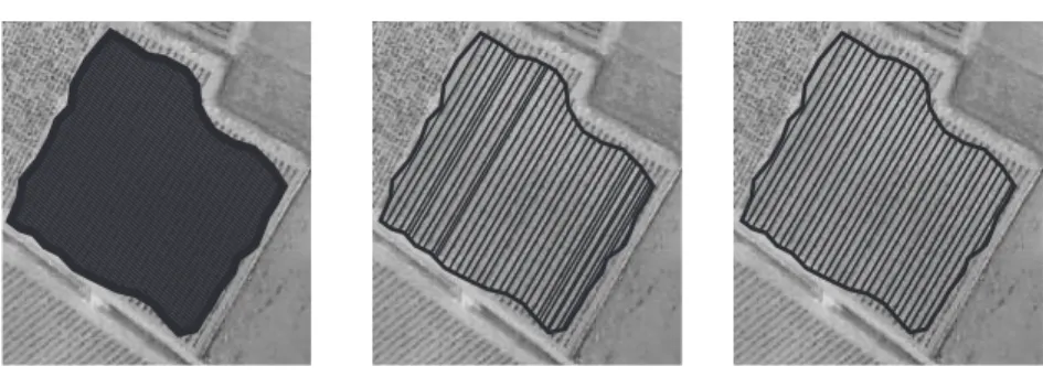
width (Figure 1).

Fig. 1. Vine row detection. Left: row network initial setting; middle: elimination of false rows using the constraint of digital number local minima; right: further elimination using the constraint of minimum interrow width.

2.3.2 Network adjustment on the parcel neighbourhood

187

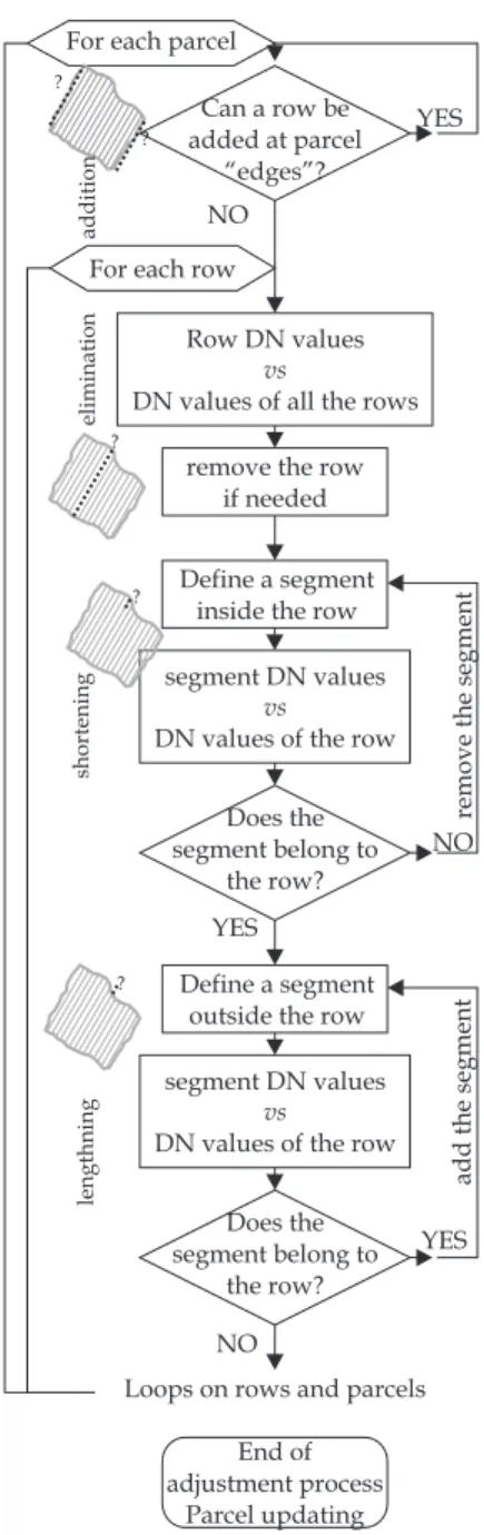
The row network is precisely adjusted using four actions: two row length ad-justments, shortening and lengthening, and two adjustments of row number, elimination and addition. In the following, the two classes ‘row’ and ‘interrow’ are considered (the interrows being defined by translating the rows of half an interrow width, perpendicularly to row orientation). The general algorithm of this adjustment process is presented in Figure 2. For row length adjustment (shortening and lengthening), one meter length segments - corresponding to the mean interplant distance along a row encountered in the study area - are considered at row ends. The mean DN of a segment is compared to the DN distribution of the entire row and to the DN distribution of the both adjacent interrows using the Mahalanobis distance (introduced by P. C. Mahalanobis in 1936) defined by equation 1:

dM =

s

(v − µ)

σ2 (1)

with v the value to test, µ and σ2

the distribution mean and variance

respec-188

tively. This distance (unlike the Euclidian one) is invariant to any change of

189

scale and gives an estimation of the possibility for an element to belong to

190

a class. Thus, if the segment mean DN is closer to the class ‘row’ than the

191

class ‘adjacent interrows’, the segment is considered to belong to the row.

192

Lengthening is first tested by adding a segment to the row until it is no more

193

classified as ‘row’. If the initial lengthening fails, segment elimination is tried.

194

Additional tests check the presence of interrow segments at both sides of the

195

row to avoid some false detection due to objects having the same range of DN

196

values as vine rows (such as trees). Once initial rows are adjusted, the next

197

step consists in row elimination or addition based on the analysis of the whole

198

row mean DN value. Concerning the elimination process, each row mean DN

199

value is compared to the global distribution of the mean DN values of all the

200

rows and interrows of the parcel. The removal occurs when the row mean DN

201

value is closer to the interrows class than the row one. The same kind of test

202

is carried out to try to add some rows at the edges of the parcel.

Fig. 2. chart of the adjustment process. 2.3.3 Parcel update in the geographical database

204

When all the rows have been adjusted, the parcel boundaries need to be

cor-205

rected accordingly. At this stage, if some rows belonging to different parcels

206

but having the same orientation and interrow width overlap each other, the

207

corresponding parcels are grouped. This enables the correction of some

over-208

segmentation cases. On the contrary, when more than three consecutive rows

209

have been eliminated, the parcel is split up into two new parcels. This

en-210

ables the correction of some under-segmentation cases. Figure 3 shows some

211

improvements of parcel delineation after row detection and adjustment (see

212

section Results for more details).

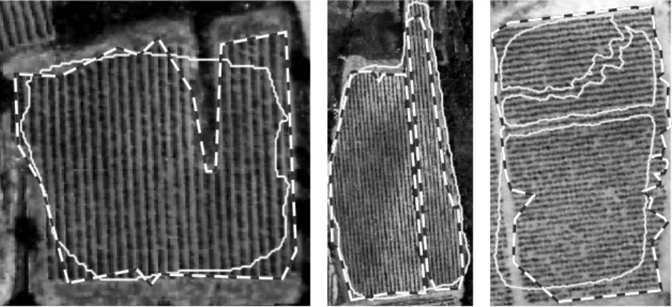
Fig. 3. Parcel boundaries improvement thanks to row adjustment (left), elimination (middle) and addition (right). Continued lines: initial boundaries; discontinued lines: adjusted ones.

2.3.4 Detection of missing vine plants

214

The missing plant detection is processed in a similar way as row length

ad-215

justment. Each row is divided in 1m length segments and the mean DN value

216

of each segment is compared to the DN distribution of the row and the both

217

adjacent interrows. When the distance to the interrow class is smaller than

218

the one to the row class, the segment is considered to correspond to a

miss-219

ing vine plant. The non-detection of missing vine plants can be due to the

220

presence of grass under the row (so that the interrow radiometry is close to

221

the row one) or to the fact that the gap has been filled by the two neighbour

222

plants. On the contrary, some plants can be wrongly considered as missing for

223

several reasons: the missing vine plant has been recently replaced and is not

224

yet visible on the image; the plant is not missing but is not very sturdy; the

225

interrow is covered by grass so that the difference between row and interrow

226

is poor. . . (see section Results for more details).

227

2.3.5 Soil surface characterization: alternation of weed control methods

228

When alternation of weed control methods is observed, another periodical

pat-229

tern appears on the image with a frequency twice or three or four times smaller

230

as the one characterizing the row (according to the combination modality).

231

To automatically assess this secondary pattern, the one dimensional Fourier

232

transform is computed for each parcel on the signal made by the interrows DN

233

means. Then, knowing the interrow frequency f , the process seeks for a second

234

local maximum and estimates its frequency f2. There will be alternation if the

235

frequency f2 is approximately equal to f /2, f /3 or f /4.

Case Meaning

1. Good segmentation The common covering surface is higher than 70% of both manually and automatically segmented parcels.

2. Over-segmentation Several parcels are automatically segmented within one real parcel.

3. Under-segmentation One automatically segmented parcel includes several real parcels.

4. Partial segmentation Only one part of the real parcel is detected.

5. Larger segmentation The automatically segmented parcel spills over one or more parcels.

6. Missing segmentation Vine parcels not automatically segmented.

7. Extra segmentation Non-vine parcels automatically segmented as vine.

8. Other cases All other cases such as both over and under segmentation or both under and partial segmentation.

Table 1

Segmentation result classification: 8 different cases can be considered. 3 Results

237

3.1 Segmentation results before and after row adjustment

238

For the validation process, the results of vine parcel segmentation are classified

239

using the 8 different cases defined in Table 1, according to their compliance

240

with the reference boundaries (see Rabatel et al. [2008] for more details).

241

Segmentation results obtained on the red channel of the image are presented

242

in Table 2 before and after row adjustment. These results have been obtained

243

with the first cited approach (Delenne et al. [2006]). As presented in Rabatel

244

et al. [2008], On the former results, only 12 parcels (10%) are not detected,

245

all of them - except one - being smaller than 0.5 ha and thus leading to weak

246

amplitude peak in the Fourier spectrum. Even the very young parcels of the

247

study area (less than three years old) have been detected, thanks to the

en-248

hancement of the image contrast. Nearly half the parcels have been correctly

249

segmented (case 1), and many have been under (14.8%) or partially segmented

250

(10.7%). As shown in the second column of Table 2, the rows detection and

251

adjustment process enhances these first results in many ways, leading to a

252

raise of correctly segmented parcel rate from 48% to 56.2%. No further

im-253

provement step can be envisaged concerning the case of missing segmentation,

254

which contains one more parcel after a too important shortening of its rows.

255

However, this case concerns less than 5% of the study area and these kinds

Case Before row adjustment After row adjustment 1. Good 58 (48 %) 68 (56.2%) 2. Over 3 (2.5%) 1 (0.8%) 3. Under 18 (14.8%) 19 (15.7%) 4. Partial 13 (10.7%) 9 (7.5%) 5. Larger 8 (6.6%) 3 (2.5%) 6. Missing 12 (10%) 13 (10.7%) 7. Extra 7 (-) 3 (-) 8. Other 9 (7.4%) 8 (6.6%) Table 2

Segmentation results (in parcel and percentage) obtained on the red channel of a 50cm resolution image, before and after row adjustment, for the 121 vine parcel of the Roujan study site.

of small parcels tends to be no more exploited due to the general increase of

257

mechanization.

258

3.1.1 Characterization results

259

3.1.1.1 Interrow width and row orientation Between on-screen

mea-260

surements and method-derived estimates, average absolute differences of less

261

than 1o

and 3.3 cm have been found respectively for row orientation and

262

interrow width. As shown in Figure 4, the coefficients of determination R2

263

obtained when comparing computed parameters to reference data are almost

264

equal to 1 for both characteristics. Moreover, it could be visually assessed in

265

the step of row extraction that the reference rows orientations (obtained by

266

photo-interpretation) are less accurate than the automatically computed ones.

267

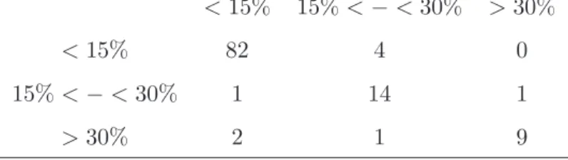
3.1.1.2 Missing vine plants detection Figure 5 shows some examples

268

of results obtained with the proposed method. An exhaustive validation could

269

not be done because of the lack of ground data. The following classification

270

(done by photo-interpretation) is thus used: (1) less than 15% of missing vine

271

plants, (2) between 15% and 30%, (3) more than 30%. The confusion matrix

272

of this classification is given in Table 3 for all the vine parcels of the study

273

area except seven very young vineyards for which vine plants are not visible

274

by photo-interpretation. These results are very satisfactory since 92% of the

275

parcels have been well classified. This kind of information will be useful for

276

vineyard managers, for example to target the parcels which will need a more

277

specific attention.

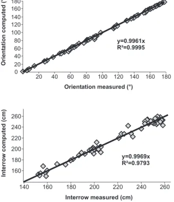
0 20 40 80 100 60 180 120 140 160 20 40 60 80 100 120 140 160 180 Orient ationcomputed(°) Orientation measured (°) y=0.9961x R²=0.9995 180 160 180 140 160 Interrowcomputed(cm) Interrow measured (cm) y=0.9969x R²=0.9793 240 200 220 260 220 200 260 240

Fig. 4. Interrow width and row orientation: on-screen measurements vs automatic estimation.

Fig. 5. Examples of missing vine plants detection. Image subsets in parcels having more than 25% (left) and less than 15% (middle) of missing plants; detection error due to the presence of grass under the row (right).

3.1.1.3 Soil surface characterization: alternation of weed control

279

methods Confusion matrix for ‘alternated parcels’ detection is given in

Ta-280

ble 4. 81% of the 121 parcels have been well classified. Nearly all the

classifica-281

tion errors concern alternated parcels for which the periodic pattern is poorly

282

contrasted in the image (Figure 6a). As a consequence, results obtained

con-283

cerning parcels with some interrows covered by grass are much satisfactory,

284

with only 4 wrong classifications over 18. The two non alternated parcels which

285

have been wrongly classified contain some interconnecting farm roads, which

286

induce a secondary and confusing pattern.

<15% 15% < − < 30% >30%

<15% 82 4 0

15% < − < 30% 1 14 1

>30% 2 1 9

Amount of correct classifications: 105/114 (92%) Table 3

Confusion matrix concerning vineyard classification in three classes according to their rate of missing vine plants (automatic process in line, photo-interpretation in column). 1/1 1/2 2/3 3/4 1/1 85 16 2 0 1/2 1 13 0 0 2/3 0 0 0 0 3/4 1 0 0 3

Amount of correct classifications: 98/121 (81%) Table 4

Confusion matrix concerning vineyard classification according to their cultural practice (alternation of weed control methods). Automatic process in line, photo-interpretation in column. 0 f original peak f/2 Amplitude Frequency FFT secondary peak

Fig. 6. Left: example of an undetected alternation 1/3 (invisible at naked eye); right: example of an alternation 1/2 and its Fourier spectrum.

4 Discussion and conclusions

288

In this study, a comprehensive process for vineyard detection, delineation and

289

intra-parcel characterization has been proposed. The main advantages of this

290

method are: its easy implementation, processing speed and the limited amount

291

of parameters. It has been implemented in a completely automatic way and

292

exports results into GIS format (.shp) with an associated database containing

293

characteristics such as area, perimeter, interrow width, row orientation,

miss-294

ing vine plants rate and cultural practices. This process, easily integrated in

295

the GIS used by vineyards managers, will enable a considerable reduction of

the cost previously needed to obtain all these characteristics using on-ground

297

surveys or photo-interpretation. Indeed, the survey done for the validation

298

of this study took two days when it only consisted in checking several

char-299

acteristics of the parcel without carrying out the differential GPS survey of

300

boundaries. Meanwhile, only about one hour is needed for the automatic

pro-301

cess on a personal computer, which may be the same for a manual digitization

302

but do not need such user intervention. Moreover, it has been shown that the

303

automatic estimation of vine row orientation and interrow width are more

ac-304

curate than those obtained by photo interpretation or ground measurements.

305

As the method description is relatively long, we have chosen to present only

306

the best results, obtained with the red channel of the image. These make us

307

confident regarding the interest of the method as only 10% of the vine parcels

308

have not been detected in the first step of segmentation, mainly concerning

309

small parcels which tend to be no longer exploited due to their inadequacy

310

with the general mechanization used in viticulture. Although not validated

311

exhaustively, the missing vine plant detection seems to be correctly assessed

312

as 92% of the parcels have been correctly classified according to three classes

313

of missing plants rate. The results of cultural practices characterization are

314

slightly poorer, except concerning practices involving grass cover. As said in

315

introduction, this information, even partial, will be useful to introduce in

dis-316

tributed hydrological models. As a perspective, a complete evaluation of the

317

method according to different types of input data (resolution, spectral bands,

318

Lidar data. . . ) will be done and presented in a further paper.

319

Acknowledgment

320

The present study has been partly carried out within the European research

321

project Bacchus (EVG2-2001-00023) with a co-funding from the European

322

Commission and within the MOBHYDIC project of the French national

pro-323

gram of research in hydrology. Aerial images were acquired by the Avion Jaune

324

company.

325

References

326

W. Bobillet, J.-P. Da Costa, C. Germain, O. Lavialle, and G. Grenier. Row

327

detection in high resolution remote sensing images of vine fields. In

328

J. Stafford and A. Werner, editors, European Conference on Precision

329

Agriculture, pages 81–87, Berlin, 2003. Wageningen academic publishers.

330

J. W. Cooley and J. W. Tukey. An algorithm for the machine calculation

331

of complex Fourier series. Mathematics of Computation, 19(90):297–301,

332

1965.

J. P. Da Costa, F. Michelet, C. Germain, O. Lavialle, and G. Grenier.

Delin-334

eation of vine parcels by segmentation of high resolution remote sensed

335

images. Precision Agriculture, 8(1):95–110, 2007.

336

C. Delenne. Extraction et caractrisation de vignes partir de donnes de

tldtec-337

tion trs haute rsolution spatiale. PhD thesis, ENGREF, 2006.

338

C. Delenne, G. Rabatel, V. Agurto, and M. Deshayes. Vine plot detection

339

in aerial images using fourier analysis. In S. Lang, T. Blaschke, and

340

E. Schpfer, editors, 1st International Conference on Object-based Image

341

Analysis (OBIA 2006), 2006.

342

C. Delenne, S. Durrieu, G. Rabatel, M. Deshayes, J.-S. Bailly, C. Lelong, and

343

P. Couteron. Textural approaches for vineyard detection and

characteriza-344

tion using very high spatial resolution remote-sensing data. International

345

Journal of Remote Sensing, 29(4):1153–1167, 2008a.

346

C. Delenne, G. Rabatel, and M. Deshayes. An automatized frequency

anal-347

ysis for vine plot detection and delineation in remote sensing. IEEE

348

Geosciences and Remote Sensing Letters, 5(3):341–345, 2008b.

349

A. Hall, J. Louis, and D. Lamb. Characterising and mapping vineyard canopy

350

using high-spatial-resolution aerial multispectral images. Computers and

351

Geosciences, 29:813–822, 2003.

352

D. W. Lamb, M. M. Weedon, and R. G. V. Bramley. Using remote sensing

353

to predict grape phenolics and colour at harvest in a Cabernet Sauvigon

354

vineyard: Timing observation against vine phenology and optimising

res-355

olution. Australian Journal of Grape and Wine Research, 10(1):46–54,

356

2004.

357

B. Lennartz, X. Louchart, M. Voltz, and Andrieux P. Diuron and simazine

358

losses to runoff water in mediterranean vineyards as related to agricultural

359

practices. Journal of Environmental Quality, 26:14931502, 1997.

360

S. Montesinos Aranda and A. Quintanilla. ”BACCHUS”: methodological

ap-361

proach for vineyard inventory and management. European Commission

362

DG Research, 2006.

363

G. Rabatel, C. Delenne, and M Deshayes. A non-supervised approach

us-364

ing gabor filters for vine-plot detection in aerial images. Computers and

365

electronics in agriculture, 62:159–168, 2008.

366

I. Takken, G. Govers, V. Jetten, J. Nachtergaele, A. Steegen, and J. Poesen.

367

Effects of tillage on runoff and erosion patterns. Soil and Tillage Research,

368

61:55–60, 2001.

369

T. Wassenaar, J.-M. Robbez-Masson, P. Andrieux, and F. Baret. Vineyard

370

identification and description of spatial crop structure by per-field

fre-371

quency analysis. International Journal of Remote Sensing, 23(17):3311–

372

3325, 2002.

373

P. J. Zarco-Tejada, A. Berj´on, R. L´opez-Lozano, J. R. Miller, P. Mart´ın, V.

Ca-374

chorro, M. R. Gonz´alez, and A. de Frutos. Assessing vineyard condition

375

with hyperspectral indices: Leaf and canopy reflectance simulation in a

376

row-structured discontinuous canopy. Remote Sensing of Environment,

377

99:271–287, 2005.