AN ALL-SKY SEARCH FOR THREE FLAVORS
OF NEUTRINOS FROM GAMMA-RAY BURSTS
WITH THE ICECUBE NEUTRINO OBSERVATORY
The MIT Faculty has made this article openly available. Please share
how this access benefits you. Your story matters.
Citation
Aartsen, M. G. et al. “AN ALL-SKY SEARCH FOR THREE FLAVORS
OF NEUTRINOS FROM GAMMA-RAY BURSTS WITH THE ICECUBE
NEUTRINO OBSERVATORY.” The Astrophysical Journal 824, 2 (June
2016): 115 © 2016 American Astronomical Society
As Published
http://dx.doi.org/10.3847/0004-637X/824/2/115
Publisher
IOP Publishing
Version
Final published version
Citable link
http://hdl.handle.net/1721.1/114032
Terms of Use
Article is made available in accordance with the publisher's
policy and may be subject to US copyright law. Please refer to the
publisher's site for terms of use.
AN ALL-SKY SEARCH FOR THREE FLAVORS OF NEUTRINOS FROM GAMMA-RAY BURSTS WITH THE
ICECUBE NEUTRINO OBSERVATORY
M. G. Aartsen1, K. Abraham2, M. Ackermann3, J. Adams4, J. A. Aguilar5, M. Ahlers6, M. Ahrens7, D. Altmann8, T. Anderson9, I. Ansseau5, G. Anton8, M. Archinger10, C. Arguelles11, T. C. Arlen9, J. Auffenberg12, X. Bai13, S. W. Barwick14, V. Baum10, R. Bay15, J. J. Beatty16,17, J. Becker Tjus18, K.-H. Becker19, E. Beiser6, S. BenZvi20, P. Berghaus3, D. Berley21, E. Bernardini3, A. Bernhard2, D. Z. Besson22, G. Binder15,23, D. Bindig19, M. Bissok12, E. Blaufuss21, J. Blumenthal12, D. J. Boersma24, C. Bohm7, M. Börner25, F. Bos18, D. Bose26, S. Böser10, O. Botner24, J. Braun6, L. Brayeur27, H.-P. Bretz3, N. Buzinsky28, J. Casey29, M. Casier27, E. Cheung21, D. Chirkin6, A. Christov30,
K. Clark31, L. Classen8, S. Coenders2, G. H. Collin11, J. M. Conrad11, D. F. Cowen9,32, A. H. Cruz Silva3, J. Daughhetee29, J. C. Davis16, M. Day6, J. P. A. M. de André33, C. De Clercq27, E. del Pino Rosendo10, H. Dembinski34,
S. De Ridder35, P. Desiati6, K. D. de Vries27, G. de Wasseige27, M. de With36, T. DeYoung33, J. C. Díaz-Vélez6, V. di Lorenzo10, H. Dujmovic26, J. P. Dumm7, M. Dunkman9, B. Eberhardt10, T. Ehrhardt10, B. Eichmann18, S. Euler24, P. A. Evenson34, S. Fahey6, A. R. Fazely37, J. Feintzeig6, J. Felde21, K. Filimonov15, C. Finley7, S. Flis7, C.-C. Fösig10,
T. Fuchs25, T. K. Gaisser34, R. Gaior38, J. Gallagher39, L. Gerhardt15,23, K. Ghorbani6, D. Gier12, L. Gladstone6, M. Glagla12, T. Glüsenkamp3, A. Goldschmidt23, G. Golup27, J. G. Gonzalez34, D. GÓra3, D. Grant28, Z. Griffith6,
C. Ha15,23, C. Haack12, A. Haj Ismail35, A. Hallgren24, F. Halzen6, E. Hansen40, B. Hansmann12, T. Hansmann12, K. Hanson6, D. Hebecker36, D. Heereman5, K. Helbing19, R. Hellauer21, S. Hickford19, J. Hignight33, G. C. Hill1, K. D. Hoffman21, R. Hoffmann19, K. Holzapfel2, A. Homeier41, K. Hoshina6,42, F. Huang9, M. Huber2, W. Huelsnitz21,
P. O. Hulth7, K. Hultqvist7, S. In26, A. Ishihara38, E. Jacobi3, G. S. Japaridze43, M. Jeong26, K. Jero6, B. J. P. Jones11, M. Jurkovic2, A. Kappes8, T. Karg3, A. Karle6, U. Katz8, M. Kauer6,44, A. Keivani9, J. L. Kelley6, J. Kemp12, A. Kheirandish6, M. Kim26, T. Kintscher3, J. Kiryluk45, S. R. Klein15,23, G. Kohnen46, R. Koirala34, H. Kolanoski36, R. Konietz12, L. Köpke10, C. Kopper28, S. Kopper19, D. J. Koskinen40, M. Kowalski3,36, K. Krings2, G. Kroll10, M. Kroll18, G. Krückl10, J. Kunnen27, S. Kunwar3, N. Kurahashi47, T. Kuwabara38, M. Labare35, J. L. Lanfranchi9, M. J. Larson40,
D. Lennarz33, M. Lesiak-Bzdak45, M. Leuermann12, J. Leuner12, L. Lu38, J. Lünemann27, J. Madsen48, G. Maggi27, K. B. M. Mahn33, M. Mandelartz18, R. Maruyama44, K. Mase38, H. S. Matis23, R. Maunu21, F. McNally6, K. Meagher5, M. Medici40, M. Meier25, A. Meli35, T. Menne25, G. Merino6, T. Meures5, S. Miarecki15,23, E. Middell3, L. Mohrmann3,
T. Montaruli30, R. Morse6, R. Nahnhauer3, U. Naumann19, G. Neer33, H. Niederhausen45, S. C. Nowicki28, D. R. Nygren23, A. Obertacke Pollmann19, A. Olivas21, A. Omairat19, A. O’Murchadha5, T. Palczewski49, H. Pandya34, D. V. Pankova9, L. Paul12, J. A. Pepper49, C. Pérez de los Heros24, C. Pfendner16, D. Pieloth25, E. Pinat5, J. Posselt19,
P. B. Price15, G. T. Przybylski23, M. Quinnan9, C. Raab5, L. Rädel12, M. Rameez30, K. Rawlins50, R. Reimann12, M. Relich38, E. Resconi2, W. Rhode25, M. Richman47, S. Richter6, B. Riedel28, S. Robertson1, M. Rongen12, C. Rott26,
T. Ruhe25, D. Ryckbosch35, L. Sabbatini6, H.-G. Sander10, A. Sandrock25, J. Sandroos10, S. Sarkar40,51, K. Schatto10, M. Schimp12, P. Schlunder25, T. Schmidt21, S. Schoenen12, S. Schöneberg18, A. Schönwald3, L. Schumacher12, D. Seckel34, S. Seunarine48, D. Soldin19, M. Song21, G. M. Spiczak48, C. Spiering3, M. Stahlberg12, M. Stamatikos16,52, T. Stanev34, A. Stasik3, A. Steuer10, T. Stezelberger23, R. G. Stokstad23, A. Stößl3, R. Ström24, N. L. Strotjohann3, G. W. Sullivan21, M. Sutherland16, H. Taavola24, I. Taboada29, J. Tatar15,23, S. Ter-Antonyan37, A. Terliuk3, G. TešiĆ9,
S. Tilav34, P. A. Toale49, M. N. Tobin6, S. Toscano27, D. Tosi6, M. Tselengidou8, A. Turcati2, E. Unger24, M. Usner3, S. Vallecorsa30, J. Vandenbroucke6, N. van Eijndhoven27, S. Vanheule35, J. van Santen3, J. Veenkamp2, M. Vehring12,
M. Voge41, M. Vraeghe35, C. Walck7, A. Wallace1, M. Wallraff12, N. Wandkowsky6, Ch. Weaver28, C. Wendt6, S. Westerhoff6, B. J. Whelan1, K. Wiebe10, C. H. Wiebusch12, L. Wille6, D. R. Williams49, L. Wills47, H. Wissing21, M. Wolf7, T. R. Wood28, K. Woschnagg15, D. L. Xu6, X. W. Xu37, Y. Xu45, J. P. Yanez3, G. Yodh14, S. Yoshida38, and
M. Zoll7
(IceCube Collaboration)
1
Department of Physics, University of Adelaide, Adelaide, 5005, Australia
2Technische Universität München, D-85748 Garching, Germany 3
DESY, D-15735 Zeuthen, Germany
4
Dept.of Physics and Astronomy, University of Canterbury, Private Bag 4800, Christchurch, New Zealand
5
Université Libre de Bruxelles, Science Faculty CP230, B-1050 Brussels, Belgium
6
Dept.of Physics and Wisconsin IceCube Particle Astrophysics Center, University of Wisconsin, Madison, WI 53706, USA
7
Oskar Klein Centre and Dept.of Physics, Stockholm University, SE-10691 Stockholm, Sweden
8
Erlangen Centre for Astroparticle Physics, Friedrich-Alexander-Universität Erlangen-Nürnberg, D-91058 Erlangen, Germany
9Dept.of Physics, Pennsylvania State University, University Park, PA 16802, USA 10
Institute of Physics, University of Mainz, Staudinger Weg 7, D-55099 Mainz, Germany
11Dept.of Physics, Massachusetts Institute of Technology, Cambridge, MA 02139, USA 12
III. Physikalisches Institut, RWTH Aachen University, D-52056 Aachen, Germany
13Physics Department, South Dakota School of Mines and Technology, Rapid City, SD 57701, USA 14
Dept.of Physics and Astronomy, University of California, Irvine, CA 92697, USA
15
Dept.of Physics, University of California, Berkeley, CA 94720, USA
16
Dept.of Physics and Center for Cosmology and Astro-Particle Physics, Ohio State University, Columbus, OH 43210, USA
17
Dept.of Astronomy, Ohio State University, Columbus, OH 43210, USA
18Fakultät für Physik & Astronomie, Ruhr-Universität Bochum, D-44780 Bochum, Germany 19
Dept.of Physics, University of Wuppertal, D-42119 Wuppertal, Germany
20
Dept.of Physics and Astronomy, University of Rochester, Rochester, NY 14627, USA
21
Dept.of Physics, University of Maryland, College Park, MD 20742, USA;hellauer@umd.edu 22
Dept.of Physics and Astronomy, University of Kansas, Lawrence, KS 66045, USA
23
Lawrence Berkeley National Laboratory, Berkeley, CA 94720, USA
24
Dept.of Physics and Astronomy, Uppsala University, Box 516, SE-75120 Uppsala, Sweden
25Dept.of Physics, TU Dortmund University, D-44221 Dortmund, Germany 26
Dept.of Physics, Sungkyunkwan University, Suwon 440-746, Korea
27Vrije Universiteit Brussel, Dienst ELEM, B-1050 Brussels, Belgium 28
Dept.of Physics, University of Alberta, Edmonton, Alberta, T6G 2E1, Canada
29
School of Physics and Center for Relativistic Astrophysics, Georgia Institute of Technology, Atlanta, GA 30332, USA
30
Département de physique nucléaire et corpusculaire, Université de Genève, CH-1211 Genève, Switzerland
31
Dept.of Physics, University of Toronto, Toronto, Ontario, M5S 1A7, Canada
32Dept.of Astronomy and Astrophysics, Pennsylvania State University, University Park, PA 16802, USA 33
Dept.of Physics and Astronomy, Michigan State University, East Lansing, MI 48824, USA
34Bartol Research Institute and Dept.of Physics and Astronomy, University of Delaware, Newark, DE 19716, USA 35
Dept.of Physics and Astronomy, University of Gent, B-9000 Gent, Belgium
36
Institut für Physik, Humboldt-Universität zu Berlin, D-12489 Berlin, Germany
37
Dept.of Physics, Southern University, Baton Rouge, LA 70813, USA
38
Dept.of Physics, Chiba University, Chiba 263-8522, Japan
39
Dept.of Astronomy, University of Wisconsin, Madison, WI 53706, USA
40
Niels Bohr Institute, University of Copenhagen, DK-2100 Copenhagen, Denmark
41
Physikalisches Institut, Universität Bonn, Nussallee 12, D-53115 Bonn, Germany
42
Earthquake Research Institute, University of Tokyo, Bunkyo, Tokyo 113-0032, Japan
43
CTSPS, Clark-Atlanta University, Atlanta, GA 30314, USA
44
Dept.of Physics, Yale University, New Haven, CT 06520, USA
45Dept.of Physics and Astronomy, Stony Brook University, Stony Brook, NY 11794-3800, USA 46
Université de Mons, B-7000 Mons, Belgium
47
Dept.of Physics, Drexel University, 3141 Chestnut Street, Philadelphia, PA 19104, USA
48
Dept.of Physics, University of Wisconsin, River Falls, WI 54022, USA
49
Dept.of Physics and Astronomy, University of Alabama, Tuscaloosa, AL 35487, USA
50
Dept.of Physics and Astronomy, University of Alaska Anchorage, 3211 Providence Dr., Anchorage, AK 99508, USA
51
Dept.of Physics, University of Oxford, 1 Keble Road, Oxford OX1 3NP, UK
52
NASA Goddard Space Flight Center, Greenbelt, MD 20771, USA
Received 2016 January 25; revised 2016 April 24; accepted 2016 April 29; published 2016 June 20
ABSTRACT
We present the results and methodology of a search for neutrinos produced in the decay of charged pions created in interactions between protons and gamma-rays during the prompt emission of 807 gamma-ray bursts(GRBs) over the entire sky. This three-year search is thefirst in IceCube for shower-like Cherenkov light patterns from electron, muon, and tau neutrinos correlated with GRBs. We detectfive low-significance events correlated with five GRBs. These events are consistent with the background expectation from atmospheric muons and neutrinos. The results of this search in combination with those of IceCube’s four years of searches for track-like Cherenkov light patterns from muon neutrinos correlated with Northern-Hemisphere GRBs produce limits that tightly constrain current models of neutrino and ultra high energy cosmic ray production in GRBfireballs.
Key words: gamma-ray burst: general – methods: data analysis – neutrinos – telescopes 1. INTRODUCTION
Ultra high energy cosmic rays(UHECRs), defined by energy exceeding 1018 eV, have been observed for decades(Zatsepin & Kuzmin1966; Abbasi et al.2008; Abraham et al.2010), but
their sources remain unknown. Gamma-ray bursts(GRBs) are among the most plausible candidates for these particles’ origins. If this hypothesis is true, neutrinos would also be produced in pg interactions at these sources. While the charged cosmic rays are deflected by galactic and intergalactic magnetic fields, neutrinos travel unimpeded through the universe and disclose their source directions. The detection of high energy neutrinos correlated with gamma-ray photons from a GRB would provide evidence of hadronic interaction in these powerful phenomena and confirm their role in UHECR production.
GRBs are the brightest electromagnetic explosions in the universe and are observed by dedicated spacecraft detectors at an average rate of about one per day (Meszaros 2006; von
Kienlin et al.2014). GRB locations are distributed isotropically
at cosmic distances. Their prompt gamma-ray emissions exhibit diverse light curves and durations, lasting from milliseconds to hours. The origins of these extremely energetic phenomena remain unknown, but their spectra have been studied extensively over a wide range of energies (Sakamoto et al.
2011; Ackermann et al.2013; Gruber et al.2014). The Fermi
detector covers seven decades of energy in gamma-rays with its two instruments and has observed photons with source-frame-corrected energies above 10 GeV early in the prompt phase of some bursts(Bissaldi et al.2015). These measurements support
efficient particle acceleration in GRBs.
The prevailing phenomenology that successfully describes GRB observations is that of a relativistically expandingfireball of electrons, photons, and protons (Piran 2004; Fox & Mészáros2006; Meszaros2006). The initially opaque fireball
plasma expands by radiation pressure until it becomes optically thin and emits the observed gamma-rays. During this
expansion, kinetic energy is dissipated through internal shock fronts that accelerate electrons and protons via the Fermi mechanism to the observed gamma-ray and UHECR energies (Waxman 1995; Vietri1997). These high energy protons will
interact with gamma-rays radiated by electrons and create neutrinos, for example, through the delta-resonance:
p+ D g + p++ n e++ne+n¯m+nm+n. ( )1 To date, no neutrino signal has been detected in searches for muon neutrinos from GRBs in multiple years of data from AMANDA, the partially instrumented IceCube, and the completed IceCube detector (Achterberg et al. 2007; Abbasi et al. 2010,2011b,2012a; Aartsen et al. 2015d), nor in four
years of data by the ANTARES collaboration (Presani 2011; Adrián-Martínez et al.2013a,2013b). High energy nm
charged-current interactions produce high energy muons that manifest as extended Cherenkov light patterns in the South Pole glacial ice, referred to as “tracks”; and Southern Hemisphere bursts were often excluded from searches for this signal in order to remove the dominant cosmic-ray-induced muon background. Adding the low-background “shower” channel from interac-tions other than charged-current nm gives enhanced sensitivity
to such bursts, improving the sensitivity of the overall correlation analysis. Both the shower and track analyses are sensitive to the combined flux of neutrinos and anti-neutrinos and are unable to distinguish between them.
This paper is ordered as follows. In Section 2, we describe the neutrino spectra predicted by the different fireball models on which we place limits. In Section 3, we describe the IceCube detector and data acquisition system. We discuss the simulation and reconstruction of events in IceCube in Section4. We detail the event selection techniques and likelihood analysis in Sections5and6. Finally, in Section7we present the results of this all-sky three-flavor shower search in combination with those from the nm track searches, and conclude in Section8.
2. PROMPT GRB NEUTRINO PREDICTIONS In this search for GRB neutrinos, we examine data during the time of gamma-ray emission reported by any satellite for each burst. We do not consider possible precursor (Razzaque et al. 2003) or afterglow (Waxman & Bahcall 2000; Murase & Nagataki 2006; Burrows et al. 2007) neutrino emission far
outside of this prompt window. In Section7we place limits on two classes of GRB prompt neutrino flux predictions: models normalized to the observed UHECRflux (Katz et al.2009) and
models normalized to the observed gamma-ray flux for each burst.
The cosmic-ray-normalized models(Waxman & Bahcall1997; Waxman2003; Ahlers et al.2011) assume that protons emitted
by GRBs are the dominant sources of the highest energy cosmic rays observed, and with these models we place limits on this assumption. The neutrino spectral break and normalization depend on the bulk Lorentz boost factorΓ and gamma-ray break energy in the GRB fireball. Typical values required for pion production lead to the emission of ∼100 TeV neutrinos. In Section 7, we place limits on the expected neutrino flux at different break energies.
The gamma-ray-normalized models (Hümmer et al. 2012; Zhang & Kumar 2013) do not relate the observed cosmic ray
flux to neutrinos produced in GRB fireballs, and with these models we place limits on internal fireball parameters. We consider three types of gamma-ray-spectrum-normalized
fireball models, calculated on a burst-by-burst basis, that differ in their neutrino emission sites. The internal shock model relates the neutrino production radius to the variability timescale of the gamma-ray light curves (Waxman & Bahcall 1997; Hümmer et al. 2012; Zhang & Kumar 2013).
The photospheric model places the radius at the photosphere through combinations of processes such as internal shocks, magnetic reconnection, and neutron-proton collisions(Rees & Mészáros 2005; Murase 2008; Zhang & Yan 2011). The
internal collision-induced magnetic reconnection and turbu-lence (ICMART) model favors a neutrino production radius ∼10 times larger than the standard internal shock model due to a Poynting-flux-dominated outflow that remains undissipated until internal shocks destroy the ordered magneticfields (Zhang & Yan2011; Zhang & Kumar2013). These models assert that
gamma-ray emission and proton acceleration occur at the same radius. This equivalence is not necessarily true for scenarios other than the single-zone internal shock model (Bustamante et al. 2015a), but allows the predicted neutrino flux to scale
linearly with the proton-to-electron energy ratio in thefireball. Additionally, the models addressed in this work do not account for a possible enhancement to the high energy neutrinoflux due to acceleration of secondary particles(Klein et al.2013; Winter et al.2014).
We calculate the per-GRB predictions normalized to the measured gamma-ray spectra numerically with a wrapper of the Monte-Carlo generator SOPHIA (Mücke Reimer et al.2014),
taking into account the full particle production chain and synchrotron losses in inelastic pg interactions. For these calculations, we parametrize the reported gamma-ray spectrum of each GRB as a broken power-law approximation of the Band function(Band et al.1993; Zhang & Kumar2013). We retrieve
GRB parameters from the circulars published by satellite detectors on the Gamma-ray Coordinates Network53 and the Fermi GBM database (Gruber et al. 2014; von Kienlin et al.
2014). We compile the relevant temporal, spatial, and spectral
parameters used in this analysis on our GRBweb database, presented on a publicly available website54(Aguilar2011). The
prompt photon emission time (T100) is defined by the most inclusive start and end times (T1 and T2) reported by any satellite. We use the most precise localization available. Following the same prescription of our previous model limit calculations(Abbasi et al.2011b,2012a; Aartsen et al.2015d),
if the fluence is unmeasured, we use an average value of 10−5erg cm−2; if the gamma-ray break energy is unmeasured, we use 200keV for T100>2 s bursts and 1000keV for
T1002 sbursts; and if the redshift is unmeasured, we use 2.15 for T100>2 sbursts and 0.5 for T1002 s bursts.
The neutrinoflux predictions depend on several unmeasured quantities; we use a variability timescale of 0.01 s and an isotropic luminosity of 1052erg cm−2 for long bursts and a variability timescale of 0.001 s and an isotropic luminosity of 1051erg cm−2 for short bursts, which are consistent with the literature (Hümmer et al. 2012; Zhang & Kumar 2013; Baerwald et al.2014). If the redshift is known for a particular
burst, we calculate the approximate isotropic luminosity from the redshift, photonfluence, and T100(Hümmer et al.2012).
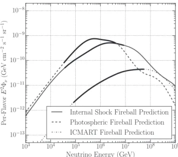
Figure1 illustrates neutrino spectra from the three models with benchmark fireball parameters. These benchmark
53http://gcn.gsfc.nasa.gov 54
parameters are bulk Lorentz boost factorG =300and proton-to-electron energy ratio, or baryonic loading, fp=10. These spectra are presented as per-flavor quasi-diffuse fluxes, in which we divide the totalfluence from all GRBs in the sample by the full sky 4p steradians and one year in seconds, and scale the total number of bursts to a predicted average 667 observable bursts per year, which has been used in our previous IceCube publications (Abbasi et al. 2010, 2011b,
2012a; Aartsen et al. 2015d). The actual number of bursts
observed by satellite detectors in each year is less than the predicted average because of detectorfield of view limitations and obstruction by the Sun, Earth, and Moon. For all GRBs we assume that neutrino oscillations over cosmic baselines result in equal fluxes for all flavors (Aartsen et al. 2015a, 2015c; Bustamante et al.2015b; Palladino et al.2015; Palomares-Ruiz et al.2015).
3. THE ICECUBE DETECTOR
The IceCube detector (Achterberg et al. 2006) consists of
5160 digital optical modules(DOMs) instrumented over 1 km3 of clear glacial ice 1450 to 2450m below the surface at the geographic South Pole. IceCube is the largest neutrino detector in operation. Each DOM incorporates a 10in. diameter photomultiplier tube (PMT) (Abbasi et al. 2010). Signal and
power connections between the DOMs and the computer farm at the surface are provided by 86 vertical in-ice cables or “strings” that each connect 60 DOMs spaced uniformly. Adjacent strings are separated by about 125 m. The DeepCore array (Abbasi et al. 2012b) is made up of a more densely
spaced subset of strings that are located in the clearest ice at depths below 2100 m and contain higher quantum ef fi-ciency PMTs.
Sensor deployment began during the 2004–2005 austral summer. Physics data collection began in 2006 with the 9-string configuration and continued with partial detector configurations through completion of the 86 strings in 2010
December. We conducted the analysis presented in this paper using data taken from 2010 May through 2013 May, with one year using the 79-string configuration and two years using the completed detector.
The DOM PMTs detect the Cherenkov radiation of relativistic charged particles produced in deep inelastic neutrino-nucleon scattering in or near the detector volume. Data acquisition (Abbasi et al. 2009) begins once the output
current exceeds the threshold of 1/4 of the mean peak current of the pulse amplified from a single photo-electron. If another such“hit” is recorded in a neighboring or next-to-neighboring DOM within 1μs, the full waveform information is recorded. DOMs with hits failing this local coincidence condition report a short summary of their recorded waveform for inclusion in data records. The digitized waveforms are sent to the computers at the surface, where they are assembled into “events” by a software trigger (Abbasi et al.2009; Kelley et al.2014). The
relative timing resolution of photons within an event is about 2ns (Achterberg et al. 2006). Data are sent daily from the
detector to computers in the Northern Hemisphere via satellite. There are two main interaction topologies that can manifest in hit DOMs during an event: a thin track or a near-spherical shower. Track-like light emission is generated by muons created either through cosmic ray interactions in the atmos-phere or nm interacting in the ice. Shower-like light emission,
which is the signal of this analysis, is generated by electromagnetic cascades from charged current interactions of
e
n and nt and hadronic cascades from neutral current interactions ofn , ne t, and nm in the ice. na stands forna+n¯a
unless otherwise specified.
Electromagnetic cascades of photons, electrons, and posi-trons develop through radiative processes, such as bremsstrah-lung and pair production. Once the energy of each particle in the cascade is below the critical energy, non-radiative processes, such as ionization and Compton scattering dominate and the shower stops growing. Hadronic cascades result from showers of baryons and mesons produced by deep inelastic scattering interactions of all neutrino types. Interactions of ¯ne
with electrons via the Glashow resonance at 6.3PeV would also produce cascade signal for this analysis; however, this resonance has not yet been observed.
4. SIMULATED DATA AND RECONSTRUCTION We use Monte Carlo simulations of neutrinos interacting in the IceCube detector for the signal hypothesis in our event selection and optimization for this search. Neutrinos are simulated with theNEUTRINO-GENERATOR program, a port of the ANIS code (Gazizov & Kowalski 2005). We use
NEUTRINO-GENERATOR to distribute neutrinos with a power-law spectrum uniformly over the entire sky and then we propagate them through the Earth and ice. The simulated neutrino-nucleon interactions take cross sections from CTEQ5 (Lai et al. 2000). The Earth’s density profile is modeled with
the Preliminary Reference Earth Model (Dziewonski & Anderson 1981). The propagation code takes into account
absorption, scattering, and neutral-current regeneration. Although we use data outside of GRB gamma-ray emission time windows for our background, simulated neutrinos and muons generated in cosmic ray air showers are useful checks to characterize our background and estimate the signal purity of our final data sample. We apply the Honda et al. spectrum (Honda et al.2007) for the atmospheric neutrino background.
Figure 1. Per-flavor quasi-diffuse all-sky flux predictions, calculated with the γ spectra of all GRBs included in this three-year search, for three different models offireball neutrino production. These fluxes assumeG =300, fp=10, fullflavor mixing at Earth, and 667 observable GRBs per year. These models differ in the radius at which pg interactions occur. The solid segments indicate the central 90% energies of neutrinos that could be detected by IceCube.
We use theCORSIKA simulation package (Heck et al.1998) to
simulate cosmic ray air showers. Muons are traced through the ice and bedrock incorporating continuous and stochastic energy losses (Chirkin & Rhode 2004). The PMT detection of
Cherenkov light from muon tracks and showers is simulated using ice and dust layer properties determined in detailed studies and simulations (Lundberg et al. 2007) (Ackermann
et al. 2006). Finally, we simulate the DOM triggering and
signal from all interactions. We process these signals in the same way as described in Section3.
We use the geometric pattern, timing, and amount of recorded photons in an interaction to reconstruct and identify the incident particle. We run simple analytic reconstructions automatically in data filters at the Pole and more complex reconstructions on the reduced data in the north. These reconstructions provide powerful discriminating features that we employ in our event selection methods, described in the next section.
One of the analytic calculations used to identify shower-like events is the “tensor-of-inertia” algorithm of Ahrens et al. (2004) that determines an interaction vertex by calculating a
“center of mass,” where the mass terms correspond to the number of photoelectrons recorded by each DOM. The eigenvector along the longest principle axis provides a reasonable guess for the incident particle trajectory. Using the rigid body analogy, a spherical shower should provide nearly even tensor-of-inertia eigenvalues, while an elongated track should have one eigenvalue much smaller than the other two.
A second analytic calculation is the “line-fit” algorithm of Ahrens et al. (2004) that ignores the geometry of the
Cherenkov cone and the optical properties of the medium and assumes light travels along a one-dimensional path at some constant velocity through the detector. This algorithm deter-mines a best-fit track, but provides a good indicator for spherical showers, which exhibit slower best-fit velocities than tracks. We recalculate this fit during the final level of event selection using an improved version of the algorithm that discards photons due to uncorrelated noise (Aartsen et al.
2014a).
We also perform fast reconstructions based on an analytic likelihood function. In general, we determine the set of parameters a={a a1, 2,¼,am} of an event that maximizes
the likelihood function
x a p x a 2 i N i 1 ( ∣ ) ( ∣ ) ( ) =
=given sets of observables x ={x x1, 2,¼,xN}from N DOMs.
We minimize the negative logarithm of with respect to a. In these online likelihood reconstructions, the x are parametrized in terms of the difference between the recorded photon hit times and the expectation without scattering or absorption (Ahrens et al.2004).
For a cascade hypothesis, which can be considered point-like because of the relatively small maximum shower range on the scale of IceCube instrumentation (Aartsen et al. 2014b), the
time residual depends on the location and time of the interaction vertex a={t x y z, , , }. This minimization is seeded by the above center of mass vertex calculation and the earliest vertex time for which at least 4 DOMs record hits with time residuals within[0, 200] ns. For an infinite track hypothesis, the time residual depends on the distance from an arbitrary point on the track and the direction of the track a={x y z, , , ,q f}. This
minimization is seeded by the above line-fit track. Both of these cascade and track hypothesis maximum likelihoods provide useful best-fit quantities for the event selection described in Section5.
The more computationally expensive likelihood-based reconstruction that we use on the reduced data takes advantage of detailed in-ice photon propagation models (Lundberg et al.
2007; Whitehorn et al.2013) and DOM waveform information.
The detection of light follows a Poisson distribution and thus the likelihood function we maximize is
k E t x y z k e , , , , , , 3 i N i k i 1 i i DOM ( ∣ ) ! ( ) q f =
l l =-for the observed and expected number of photoelectrons k and λ in each DOM from a neutrino traveling in direction (q, )f and
depositing energy E at time t and vertex x y z( , , )(Aartsen et al.
2014b). This likelihood generally considers multiple light
sources, e.g., for stochastic muon losses along a path through the detector. Because we define our signal to be neutrino-induced showers, it is sufficient to use a point-like hypothesis. Due to the linear relationship between Cherenkov light emission and deposited energy in n charged-current interac-e
tions, we estimate the electromagnetic-equivalent energy of an event by comparing to a template electromagnetic cascade of 1 GeV (Aartsen et al. 2014b). By using Cherenkov light
source-dependent spline-fit tables of photon amplitudes and time delays, we minimize (James & Roos 1975) the negative
log-likelihood and extract the best-fit parameters of the particle that produced the shower.
We iterate this minimization several times and achieve improved angular reconstruction from the best-fit energy and modeled ice structure. The reconstruction is seeded by the tensor-of-inertia direction, online likelihood vertex, and best-fit energy from a simple isotropic shower and coarsely binned propagation model expectation in Equation (3). We use this
reconstruction’s best-fit direction and energy for each event in our likelihood analysis. We estimate a lower bound on the error in the reconstructed directions with the Cramer–Rao relation (Cramer 1945; Rao1945) between the covariance of each fit
parameter and the inverted Fisher information matrix. Figure2
shows the angular and energy resolutions using this reconstruc-tion at the final event selection of this cascade search. The reconstructed energy for neutral current interactions is less than the primary neutrino energy because of the dissipation to outlets without Cherenkov emission.
5. EVENT SELECTION
Our signal in this search is one or more high energy neutrino-induced showers coincident in space and time with one or more GRBs. Before we analyze the likelihood that an event is a GRB-emitted neutrino, we must reduce the triggered data that are dominated by nearly 3 kHz of cosmic ray air shower muons to a much smaller selection of possible signal. Our event selection is optimized on a general E-2spectrum of
diffuse astrophysical simulatedn for signal and off-time datae
for background; we choose “off-time” as data not within two hours of any reported GRB γ emission in order to ensure blindness to potential signal. We use the reconstructions detailed in Section4to remove the background and realize our final sample.
Searches for neutrino-induced showers from astrophysical and atmospheric sources have been conducted previously in IceCube (Abbasi et al. 2011a; Aartsen et al. 2014c, 2014e,
2015b). The predominant difference between these and the
search presented in this paper is that we assume neutrinos come from known transient sources. The previous shower-like event selections assume a diffuse signal or constantly emitting sources, and, as a result, require much more stringent background reduction that leads to data rates nearly a factor of 100 smaller than what is needed in this search. Cascade containment constraints in the detector were imposed to reach these low backgrounds, which are achieved in this search by the effective cuts in time and space around each GRB in the unbinned likelihood analysis presented in Section6.
Thefirst class of background to remove is track-like events generated by muons losing their energy through continuous ionization processes. These muon tracks are relatively easily separated from our shower-like neutrino signal by use of afilter run online at the detector site. During the 79-string con figura-tion, we use the tensor-of-inertia eigenvalue ratio and line-fit absolute speed to choose spherical events. The online cascade filter for the first two years of the 86-string configuration imposes a zenith-dependent selection to allow more events with energies below 10 TeV. We use the reduced log-likelihood calculated in the fast cascade likelihood reconstruction to remove a large fraction of the muons that are misreconstructed as upgoing. The down-going region requires more restrictive reduced log-likelihood values in combination with the same online 79-string event selection from above.
Upon transmission via satellite from the South Pole, these ∼30Hz filtered data of spherically shaped events must be further reduced to have optimal performance with the boosted decision tree (BDT) forest algorithm described below. The background at this rate is still dominated by atmospheric muons that lose their energy through bremsstrahlung, photo-nuclear interactions, and pair production. These stochastic energy loss mechanisms create nearly spherical hit patterns that are difficult to differentiate from our signal when the muon track is at the edge or outside of the detector and therefore not observed. We derive variables from the more CPU-intensive reconstructions run offline to separate these muons from neutrino-induced showers at this selection level, called level 3 in this text, and for eventual machine-learning input.
Even though the background muons in the onlinefilter event selection are shower-like in topology, we exploit the
Cherenkov light hit patterns of the minimally ionizing muon track when possible to differentiate from showers produced by neutrinos. We perform this further separation of signal from muon background first by using the fast track hypothesis and cascade hypothesis analytic likelihood function reconstruc-tions, described in Section4. Ourfirst level 3 selection is on events for which the ratio of the track likelihood to the cascade likelihood heavily favors the cascade hypothesis. Two other background muon features that we take advantage of are their down-going directions and typically lower energies. We thus parametrize the track likelihood reconstructed zenith in terms of reconstructed energy and remove low energy down-going events from our sample. Lastly, at this rate, we choose events based on the fraction of hit DOMs that are inside of a sphere centered on the reconstructed vertex with a radius determined by the mean hit distance. We optimize the radius and fraction filled of the sphere for reconstructed vertices inside and outside of the instrumented volume and use both volume regions for this neutrino search.
Our final event selection employs a machine learning algorithm to optimize the separation of signal and background over a space of many features. The algorithm we use is a BDT forest (Freund & Schapire 1997) that also has been used in
Northern Hemisphere nm track GRB coincidence searches in IceCube(Abbasi et al.2012a; Aartsen et al.2015d). We built a
collection of variables, many of which were influenced by past neutrino-induced shower searches conducted in IceCube (Abbasi et al. 2011a; Aartsen et al. 2014c), to train the BDT
to discriminate between signal and background events. During this training, the algorithm determines the variable value that best separates signal and background at each node of each tree. Each successive tree increases, or “boosts,” the weights of incorrectly classified events from the prior tree, allowing more ambiguous events to be classified correctly. The trees and forest grow until certain stopping criteria are reached. The signal/background(+ - score of each event that we use in1 1) ourfinal selection is a weighted average of its scores over all trees, where this weight is related to the boost factor of each tree. For each of the three year-long detector configurations of this search, we train a separate BDT with configuration-specific signal simulation and background data.
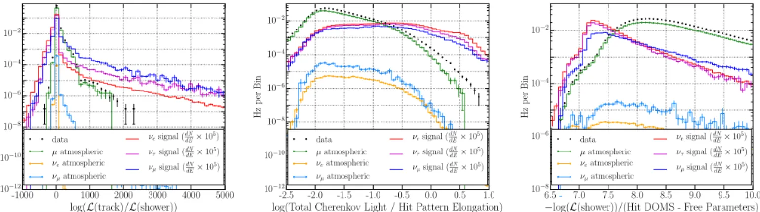
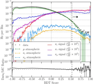
Our BDT discrimination variables take advantage of topological and energetic differences between astrophysical neutrino and atmospheric muon spectra. Figures3and4show the distributions for simulated astrophysical neutrinos,
Figure 2. Left: cumulative point-spread function per neutrino flavor at final cascade event selection. Middle: energy resolution per neutrino flavor for charged-current interactions atfinal event selection. Right: energy resolution per neutrino flavor for neutral-current interactions at final event selection.
atmospheric neutrinos, atmospheric muons, and data for three of the most powerful variables used by the BDT after level 3 and the final level, respectively. Some deviations in variable values between measured and simulated data are visible in Figures 3 and4, and are attributed to the simulation’s limited ability to produce all observed events. These deviations do not affect the analysis because the background is determined from measured data.
Figure5shows the distributions of simulation and data with respect to BDT score. The vertical dashed line corresponds to our optimized final event selection described in the next section. The atmospheric and astrophysical nm in these plots is already preselected to be shower-like and has minimal overlap with the track search. Background is reduced by a factor of 6´10-6 from the online filter level to the BDT-based final
selection. Figure 6 shows then signal efficiency at this finale
level with respect to the online filter rate as a function of energy. The slight decrease in efficiency for the highest energy signal is due to events for which the computationally expensive reconstruction, described at the end of Section4and used in the likelihood analysis, fails to converge. These simulated neutrinos interact outside of the detector, account for about 1% of the E-2 signal, and are discarded prior to the BDT
selection.
One of the most effective BDT variables is the same ratio of the track likelihood to the cascade likelihood used in level 3. The high energy background muons that passed in spite of the selection at level 3 are distinguished from signal with the BDT algorithm. The large likelihood ratios, seen in Figures3and4,
are due to the highest energy signal events with the most hit DOMs. Another potent variable is the total amount of Cherenkov light imparted in the DOMs divided by the tensor-of-inertia derived elongation of an event. The numerator separates lower energy background atmospheric muons from higher energy astrophysical signal neutrinos, while the denominator separates elongated background atmospheric muons from spherical neutrino-induced showers. As shown in Figure 3, the ratio of these two observables effectively separates the lower energy atmospheric neutrino background from our signal as well. A third useful variable is the reduced negative log-likelihood value from the analytic cascade hypothesis reconstruction.
Compared to the event samples of IceCube’s searches for
nm-induced tracks from Northern Hemisphere GRBs, our backgrounds in this all-sky all-flavor cascade search require an event selection to a 10 times lower data rate of 0.16mHz averaged over the three search years. The differences between neutrino-induced showers and muon-induced stochastic energy loss showers are less apparent than the differences between neutrino-induced tracks and detector-edge and coincident muon-induced tracks incorrectly reconstructed as upgoing. In the Northern Hemisphere track searches, most of these muons are able to be identified and removed, leaving only atmospheric neutrinos. As a result, the atmospheric neutrino purity with respect to muons of this all-sky all-flavor search is ∼40%, and is significantly less than the ∼90% purity of the Northern Hemisphere track searches. Nevertheless, we achieve similar sensitivity to the track search through our acceptance ofn , ne t,
Figure 3. Distributions for three of the most powerful signal/background discrimination variables used by the BDT forest, shown after the level 3 event selection. E-2
e
n (red solid line) was used for signal and data (black dots) were used for background in the BDT forest training.dN
dE is defined in Figure5.
Figure 4. Distributions for three of the most powerful signal/background discrimination variables used by the BDT forest, shown after the final event selection. E-2
e
n (red solid line) was used for signal and data (black dots) were used for background in the BDT forest training.dN
and nm signal from GRBs over the entire sky. Figure 7
compares the effective areas for the two different GRB neutrino searches.
6. UNBINNED LIKELIHOOD ANALYSIS
Once we have selected a sample of events that resemble high energy neutrino-induced electromagnetic or hadronic showers, we must calculate the likelihood that these events are neutrino signal from observed GRBs. We use a likelihood function that incorporates the probabilities that an event is a signal neutrino from a GRB or a background atmospheric neutrino or muon.
We calculate these background-like and signal-like probabil-ities from individually normalized probability distribution functions(PDFs) in time, space, and energy:
xi Ps ti P ri P Ei Time s Space s Energy ( ) ( ) ( ) ( ) = ´ ´ xi Pb ti P ri P E ,i Time b Space b Energy ( ) ( ) ( ) ( ) = ´ ´
where S and B are the probabilities that an event i with properties xi is signal and background, respectively.
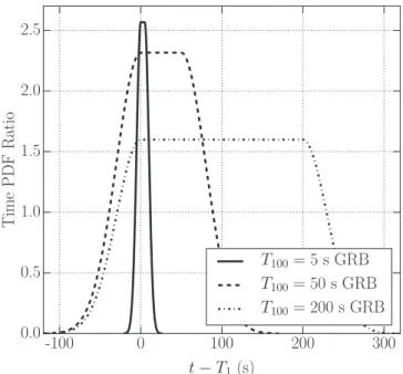
The signal time PDF isflat during the gamma-ray emission duration (T100 defined in Section 2) and has Gaussian tails before T1 and after T2. The width of these Gaussian tails st
equals the duration of measured gamma-ray emission up to 30 s and down to 2 s to account for possible small shifts in the neutrino emission time with respect to that of the photons. We accept events out to T1004st for each GRB time window.
The background time PDF isflat throughout the total period of acceptance for each GRB. Examples of the signal/background time PDF ratios for events during GRBs with different measured durations are shown in Figure8.
The signal space PDF is thefirst-order non-elliptical term in the Kent distribution(Kent1982):
r P e 4 sinh , 4 i r r sSpace( ) i GRB ( ) ( ) ( ˆ · ˆ ) k p k = k
for which the concentration parameter 1
i GRB
2 2
k =
s +s is the
reciprocal of the uncertainty in the GRB’s localization and the Cramer–Rao uncertainty in the event’s reconstructed direction,
rˆ is the reconstructed direction of the event, and ri ˆGRB is the
most precise GRB localization available. We use this spherical analog of the planar Gaussian distribution because of the large uncertainties in our reconstructed cascade event directions. The background space PDF is a spline fit to the distribution of reconstructed cos(qzenith)of allfinal analysis level off-time data
events. Small variance in the background reconstructed azimuth distribution has negligible impact on this analysis, so our background space PDF only varies with zenith. Examples of the signal space PDFs for events and correlated GRBs with different directional uncertainties are shown with the back-ground space PDF in Figure9.
The signal and background energy PDFs are the recon-structed energy distributions of E-2
e
n simulation and off-time
data, respectively. We fit a spline to the ratio of these two PDFs. Wefind few background events in our final sample that have reconstructed energies above 1 PeV, so we conservatively assume a constant ratio of signal and background energy PDFs at energies above 1 PeV. The signal and background energy PDFs and their spline-fit ratio are shown in Figure10.
In order to choose our optimalfinal selection on BDT score and characterize the significance of the result, we construct a test statistic in the form of a maximum likelihood function. This function incorporates probabilities that observed events are signal and background and provides an estimator for the number of observed signal events. The likelihood function combines the above signal and background PDFs with the Poisson probability PN of observing N events, given that the expected total number of signal + background events is
ns+nb: xi ;n n PN p x p x , 5 i N i i s b 1 s b ({ } ) ( ( ) ( )) ( ) + =
+ =Figure 5. Distribution of data, simulated muon background, simulated atmospheric neutrino background, simulated E-2 neutrino signal (where
10 GeV cm s sr dN dE E 8 1 2 1 1 GeV 2
( )
= - - - -) with respect to BDT score. The
vertical dashed line represents thefinal event selection of 0.525> .
Figure 6. Signal efficiency relative to online filter level as a function of neutrino energy. Signal is E-2
e
n simulation. Averaged over the three search years, the onlinefilter level data rate is 30 Hz and is reduced to 1.6´10-4Hz
where P n n e N 6 N N n n s b s b ( ) ! ( ) ( ) = + - + and p n n n s s s b = + and p n n n b b s b
= + are the probabilities of observing a signal and background event.
We do not know a priori the total number of events we will observe. Therefore, we estimate nbfrom the background data rate multiplied by the total search time window
T 8 i N i i 100, t, GRBs( s )
å + in which we accept events; and this expectation is denoted by ná ñ. We estimate nb sfrom the value nˆs
that maximizes . Additionally, we simplify the likelihood function by dividing by its background-only hypothesis and taking the logarithm of this ratio without loss of generality.
Finally, our test statistic T is the maximized value of this ratio at nˆ :s x x T n n n ln 1 . 7 i N i i s 0 s b ˆ ˆ ( ) ( ) ( )
å
= - + á ñ + = ⎡ ⎣ ⎢ ⎤ ⎦ ⎥We extend to multiple detector configurations (79 strings, first year of 86 strings, second year of 86 strings, etc.) and search channels(cascades, tracks) by adding maximized test statistics for each configuration and channel:
x x T n n n ln 1 , 8 i N i i c s c 0 s c c b c c c ( ˆ ) ( ˆ ) ( ) ( ) ( )
å
å
= - + á ñ + = ⎪ ⎪ ⎧ ⎨ ⎩ ⎡ ⎣ ⎢ ⎤ ⎦ ⎥⎫⎬ ⎭where c represents each combination of search channel and detector configuration.
To set discovery significance thresholds, we first perform 108pseudo-search trials using only background data for a range of BDT score> cuts. Each background sample has its owns
nb cut
á ñ , with lower values for cuts on higher BDT scores. In each background-only trial, for each GRB, we choose a pseudo-random number of observed events within our
T1004stsearch time window about the gamma-ray emission
from a Poisson distribution with expectation determined by the background data rate and time window. If the number of events is 0, then T receives no contribution from the search window about that GRB. If the number of events is greater than 0, then we construct each event using the following steps:(1) choose a random time PDF value;(2) choose a random azimuth within 0 to 2 ;p (3) choose a reconstructed energy by sampling from the background distribution;(4) choose a reconstructed zenith by sampling from the background distribution of events with similar energy; (5) choose an estimated error in reconstructed direction by sampling from the background distribution of events with similar energy and zenith. Finally, with the signal and background PDF values for every event, we calculate the test statistic for each trial. We obtain a distribution like that shown in Figure11for each possible selection on BDT score. We choose our optimal final selection on BDT score by injecting simulated neutrino signal along with background data and performing 104 pseudo-search trials for a range of BDT score> cuts. The background events are selected for eachs
GRB the same as above for the background-only trials. The simulated signal events within an 11° circle about each GRB contribute to the likelihood with a probability proportional to their simulated weight. Signal is increasingly weighted until a defined discovery or limit-setting threshold is reached. These discovery and limit-setting potentials per cut on BDT score are shown in Figure12for a general E-2spectrum and the Figure1
benchmark internal shockfireball spectrum. The final selection, BDT score >0.525, was optimized to set the best possible upper limit while suffering little loss in discovery potential. This optimization was performed for each search year’s event selection.
7. RESULTS
In three years of data,five cascade neutrino candidate events are correlated with five GRBs. These coincidences yield a combined P-value of 0.32, derived from the total test statistic value with respect to the background-only distribution. The Northern Hemisphere track searches in four years of data resulted in a single neutrino candidate event correlated with
Figure 7. Effective areas for the full-sky shower-like and Northern Hemisphere track-like GRB-coincident event searches with the 79-string detector. 79- and 86-string detector effective areas are similar.
Figure 8. Signal/background time PDF ratios for events during example GRBs with different measured T100values.
prompt GRB emission and a combined P-value of 0.46 (Aartsen et al. 2015d). Considering the atmospheric neutrino
purity of each search, discussed in Section5, the track event is almost certainly a nm while the cascade events could be high
energy atmospheric muons.
Table 1 shows the time, space, and energy data for these events and GRBs. Events 1, 2, and 4 occurred on the edge or corner of the detector. Events 3 and 5 occurred within the instrumented volume. The large directional uncertainties of the second and fourth events are due to the location of their interactions at the corner and edge of the instrumented volume, with relatively few DOMs able to record the Cherenkov light. The reconstructed energy of the muon neutrino track coincidence discussed in Aartsen et al. (2015d) is an
approximate lower bound on the neutrino energy because the interaction could have taken place well outside of IceCube and
consequently, the muon could have lost significant energy before reaching the detector.
The benchmark internal shock, photospheric, and ICMART fireball model spectra plotted in Figure1yield expectations of 1.5, 2.5, and 0.07 neutrinos, respectively, for this three-year all-flavor cascade analysis. As discussed at the end of Section5, this search achieves nearly the same sensitivity as the Northern Hemisphere track search. Thus, the combined four years of track searches and three years of shower searches yield total benchmark model expectations of 3.3, 5.4, and 0.1 neutrinos. The all-flavor shower search has an average ná ñ of 11 eventsb
per year. This expectation is more concentrated at lower energies than the expected signal and is weighted by the time, space, and energy PDFs accordingly in our unbinned like-lihood. The expected background during just the T100of each
Figure 9. Left: signal space PDFs for three example events and correlated GRBs. Right: background space PDF, calculated from a spline fit to the zenith distribution of data events at thefinal analysis level. The 79- and 86-string detectors show azimuthal symmetry.
Figure 10. Left vertical axis: Reconstructed energy distributions of data (dot markers) and E-2n signal (red line) at the final analysis level. Right verticale
axis: Signal/background energy PDF distribution (black line) calculated from a
splinefit to the ratio of the two energy distributions. Figure 11. Test statistic distribution for 10 8
randomized background-only pseudo-searches atfinal analysis level. The vertical lines represent test statistic values for a 3s, 4s, and 5s discovery.
GRB is 3.5 events per year. An observation of three 1 PeV neutrinos correlated with three GRBs, with the same temporal and spatial properties as our observed Event 1 and its respective GRB in Table 1, would yield a T value over 12 and a 5s discovery based on the background-only distribution in Figure11.
Considering the low significance of the events correlated with GRBs, we set 90% confidence level (CL) Neyman upper limits (Neyman 1937) on models normalized to the observed
flux of UHECRs as well as models normalized to the observed gamma-rayfluence of each GRB. We calculate these limits by combining the three-year cascade search results and four-year Northern Hemisphere track search results using the multiple configuration and channel test statistic given in Equation (8).
Simulated neutrinos are weighted to a certain spectrum and normalization and injected over background in the pseudo-searches. The exclusion CL is the fraction of pseudo-search trials that yield TTobserved.
Figure 12. Limit setting and discovery potentials per cut on BDT score for a single year’s search. The horizontal axes correspond to a BDT score> scut. Thefinal event selection was optimized for limit setting and suffered little loss in discovery potential. The vertical dashed line represents ourfinal event selection of BDT score
0.525
> . Left: the vertical axis corresponds to the E-2spectrum signal weight needed in order to reach the given threshold. Right: the vertical axis corresponds to the
multiplying factorμ on the benchmark internal shock fireball model neutrino flux shown in Figure1in order to reach the given threshold. Table 1
GRB and Event Properties for the Three-year Cascade and Four-year Track Search Coincidences
Time Angular Uncertainty Angular Separation Fluence/Energy
GRB 101213A T100=202 s 0 . 0005 7.4´10-6erg cm−2 Event 1 T1+109 s 32 . 0 23° 11 TeV GRB 110101B T100=235 s 16 . 5 6.6´10-6erg cm−2 Event 2 T1+141 s 118° 112° 34 TeV GRB 110521B T100=6.14 s 1 . 31 3.6´10-6erg cm−2 Event 3 T1+0.26 s 16 . 5 35° 3.4 TeV GRB 111212A T100=68.5 s 0 . 0004 1.4´10-6erg cm−2 Event 4 T1+11.7 s 44 . 8 120° 31 TeV GRB 120114A T100=43.3 s 0 . 04 2.4´10-6erg cm−2 Event 5 T1+57.2 s 7 . 9 18° 3.8 TeV GRB 100718Aa T 39 s 100= 10 . 2 2.5´10-6erg cm−2
nmTrack Eventa T1+15 s 1 . 3 16° 10 TeV
Note.
a
Corresponds to the nmtrack search coincidence discussed in Aartsen et al.(2015d).
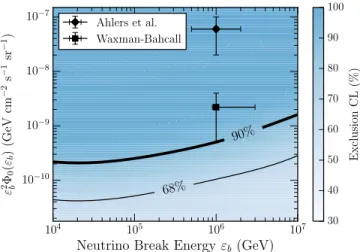
Figure 13. Exclusion contours, calculated from the combined three-year all-skyn ne tnmshower-like event search and four-year Northern Hemisphere nm
track-like event search results, of a per-flavor double broken power law GRB neutrinoflux of a given flux normalizationf at first break energy0 b.
Figure 13 shows exclusion contours for double broken power law spectra of the form
E E E E E E E , , 10 10 , 10 9 b b b b b b 0 1 1 2 4 2 ( ) ( ) ( ) f F = ´ < < n - -⎧ ⎨ ⎪ ⎩ ⎪
at differentfirst break energiesband normalizations b
2 0
f . Our
combined limits largely rule out cosmic ray escape via neutron production (Ahlers et al. 2011). Mechanisms allowing for
cosmic ray escape via protons (Waxman & Bahcall1997) are
disfavored as well. The Waxman & Bahcall(1997) model has
been updated to account for more recent measurements of the UHECR flux (Katz et al. 2009) and typical gamma break
energy (Goldstein et al.2012).
Figure14shows exclusion contours in the baryonic loading —bulk Lorentz factor parameter space for the internal shock, photospheric, and ICMART per-burst gamma-ray-normalized fireball models. The benchmark model spectra from Figure 1
are indicated by the intersection of the vertical and horizontal dashed lines. Systematic uncertainties in the ice model, DOM photon detection efficiency, and lepton propagation in the Earth and ice are added in quadrature to a total effect of~11% for each model limit. The addition of the all-sky cascade search over three years of data and GRBs improves the Northern Hemisphere track search limits by about 50%.
8. CONCLUSIONS AND OUTLOOK
We have performed a search for neutrinos of all flavors emitted by 807 GRBs during 3 years of IceCube data. This search exhibits similar sensitivity to that of previously published searches for muon neutrinos emitted by 506 Northern Hemisphere GRBs during 4 years of IceCube data. Over both search channels, we found six events that are correlated with GRBs but also consistent with background. Our limits placed on neutrino emission models normalized to the observed UHECRflux are the strongest constraints thus far on the hypothesis that GRBs are the dominant sources of thisflux. Additionally, our limits placed on the latest neutrino emission models normalized to the observed gamma-ray fluence from each GRB constrain parts of the parameter space relevant for the production of UHECR protons. Models that are still allowed require increasingly lower neutrino production ef fi-ciencies through large bulk Lorentz boost factors, low baryonic loading, or large dissipation radii.
As shown in Baerwald et al. (2014), constraints on
parameters involved infireball neutrino production via internal shock collisions can be connected to the requirement that GRBs are the sources of the observed UHECRs in a self-consistent way, assuming a pure proton composition. While cosmic ray escape from GRB fireballs through neutron production is strongly constrained by our limits, Baerwald et al. (2014) show that the unexcluded parameter space in
Figure14allows for efficient diffusive proton escape assuming a galactic-to-extragalactic source transition at the ankle of the cosmic ray spectrum. Although the allowed parameter space of this model is plausible, the average burst likely exhibitsΓ and fp values that are largely excluded for neutrino production. Nevertheless, we have only considered single-zone neutrino and cosmic ray emission models of GRBs in this work, and models of multiple emission regions predict a neutrino flux below our current sensitivity(Bustamante et al.2015a; Globus et al.2015).
Our acceptance of possible prompt neutrino signal can increase further through the addition of searches for nm-induced tracks correlated with Southern Hemisphere GRBs that occurred during the 79-string and completed detector con fig-urations. Moreoever, the next-generation IceCube-Gen2 detec-tor will significantly improve the sensitivity to transient sources (Aartsen et al.2014d; Ahlers & Halzen 2014). The continued
pursuit of all neutrino flavors from observed GRBs over the entire sky will either reveal a flux that is still lower than our current sensitivity or increasingly disfavor these phenomena as sources of the highest energy cosmic rays.
We acknowledge the support from the following agencies: the U.S. National Science Foundation-Office of Polar Pro-grams, the U.S. National Science Foundation-Physics Division, the University of Wisconsin Alumni Research Foundation, the Grid Laboratory Of Wisconsin(GLOW) grid infrastructure at the University of Wisconsin—Madison, the Open Science Grid (OSG) grid infrastructure; the U.S. Department of Energy, and the National Energy Research Scientific Computing Center, the Louisiana Optical Network Initiative (LONI) grid computing resources; the Natural Sciences and Engineering Research Council of Canada, WestGrid and Compute/Calcul Canada; the Swedish Research Council, the Swedish Polar Research Secretariat, the Swedish National Infrastructure for Computing (SNIC), and the Knut and Alice Wallenberg Foundation, Sweden; the German Ministry for Education and Research (BMBF), Deutsche Forschungsgemeinschaft (DFG), the
Figure 14. Exclusion contours, calculated from the combined three-year all-skyn ne tnmshower-like event search and four-year Northern Hemisphere nmtrack-like event search results, in fpandΓ GRB parameter space, for three different models of fireball neutrino production. These models differ in the radius at which pg interactions occur. The vertical and horizontal dashed lines indicate the benchmark parameters used for Figure1and the right panel of Figure12. Left: internal shock. Middle: photospheric. Right: ICMART.
Helmholtz Alliance for Astroparticle Physics (HAP), the Research Department of Plasmas with Complex Interactions (Bochum), Germany; the Fund for Scientific Research (FNRS-FWO), the FWO Odysseus programme, Flanders Institute to encourage scientific and technological research in industry (IWT), the Belgian Federal Science Policy Office (Belspo); University of Oxford, United Kingdom; the Marsden Fund, New Zealand; the Australian Research Council; the Japan Society for Promotion of Science (JSPS); the Swiss National Science Foundation (SNSF), Switzerland; the National Research Foundation of Korea(NRF); and the Danish National Research Foundation, Denmark(DNRF).
REFERENCES
Aartsen, M., Abbasi, R., Abdou, Y., et al. 2014a,NIMPA,736, 143 Aartsen, M., Abbasi, R., Ackermann, M., et al. 2014b,JInst,9, P03009 Aartsen, M., Abbasi, R., Ackermann, M., et al. 2014c,PhRvD,89, 102001 Aartsen, M., Abraham, K., Ackermann, M., et al. 2015a,ApJ,809, 98 Aartsen, M., Ackermann, M., Adams, J., et al. 2014d, arXiv:1412.5106 Aartsen, M., Ackermann, M., Adams, J., et al. 2014e,PhRvL,113, 101101 Aartsen, M., Ackermann, M., Adams, J., et al. 2015b,PhRvD,91, 022001 Aartsen, M., Ackermann, M., Adams, J., et al. 2015c,PhRvL,114, 171102 Aartsen, M., Ackermann, M., Adams, J., et al. 2015d,ApJL,805, L5 Abbasi, R., Abdou, Y., Abu-Zayyad, T., et al. 2010,ApJ,710, 346 Abbasi, R., Abdou, Y., Abu-Zayyad, T., et al. 2011a,PhRvD,84, 072001 Abbasi, R., Abdou, Y., Abu-Zayyad, T., et al. 2011b,PhRvL,106, 141101 Abbasi, R., Abdou, Y., Abu-Zayyad, T., et al. 2012a,Natur,484, 351 Abbasi, R., Abdou, Y., Abu-Zayyad, T., et al. 2012b,APh,35, 615 Abbasi, R., Abu-Zayyad, T., Allen, M., et al. 2008,PhRvL,100, 101101 Abbasi, R., Ackermann, M., Adams, J., et al. 2009,NIMPA,601, 294 Abbasi, R., Abdou, Y., Abu-Zayyad, T., et al. 2010,NIMPA,618, 139 Abraham, J., Abreu, P., Aglietta, M., et al. 2010,PhLB,685, 239 Achterberg, A., Ackermann, M., Adams, J., et al. 2006,APh,26, 155 Achterberg, A., Ackermann, M., Adams, J., et al. 2007,ApJ,664, 397 Ackermann, M., Ahrens, J., Bai, X., et al. 2006,JGR,111, D13203 Ackermann, M., Ajello, M., Asano, K., et al. 2013,ApJS,209, 11 Adrián-Martínez, S., Albert, A., Al Samarai, I., et al. 2013a,A&A,559, A9 Adrián-Martínez, S., Al Samarai, I., Albert, A., et al. 2013b,JCAP,1303, 006 Aguilar, J. A. 2011, Proc. ICRC, Vol. 8, Cosmic Ray Origin and Galactic
Phenomena, 235
Ahlers, M., Gonzalez-Garcia, M., & Halzen, F. 2011,APh,35, 87 Ahlers, M., & Halzen, F. 2014,PhRvD,90, 043005
Ahrens, J., Bai, X., Bay, R., et al. 2004,NIMPA,524, 169 Baerwald, P., Bustamante, M., & Winter, W. 2014,APh,62, 66 Band, D., Matteson, J., Ford, L., et al. 1993,ApJ,413, 281
Bissaldi, E., Longo, F., Omodei, N., Vianello, G., & von Kienlin, A. 2015, arXiv:1304.5570
Burrows, D. N., Falcone, A., Chincarini, G., et al. 2007,RSPTA,365, 1213 Bustamante, M., Baerwald, P., Murase, K., & Winter, W. 2015a, NatCo,
6, 6783
Bustamante, M., Beacom, J. F., & Winter, W. 2015b,PhRvL,115, 161302 Chirkin, D., & Rhode, W. 2004, arXiv:hep-ph/0407075
Cramer, H. 1945, Mathematical Methods of Statistics(Princeton, NJ: Princeton Univ. Press)
Dziewonski, A. M., & Anderson, D. L. 1981,PEPI,25, 297 Fox, D. B., & Mészáros, P. 2006,NJPh,8, 199
Freund, Y., & Schapire, R. E. 1997,J. Comput. Syst. Sci., 55, 119 Gazizov, A., & Kowalski, M. 2005,CoPhC,172, 203
Globus, N., Allard, D., Mochkovitch, R., & Parizot, E. 2015, MNRAS, 451, 751
Goldstein, A., Burgess, J., Preece, R., et al. 2012,ApJS,199, 19
Gruber, D., Goldstein, A., Weller von Ahlefeld, V., et al. 2014,ApJS,211, 12
Heck, D., Knapp, J., Capdevielle, J. N., Schatz, G., & Thouw, T. 1998, CORSIKA: A Monte Carlo Code to Simulate Extensive Air Showers, Tech. Rep. FZKA 6019, Forschungszentrum Karlsruhe
Honda, M., Kajita, T., Kasahara, K., Midorikawa, S., & Sanuki, T. 2007,
PhRvD,75, 043006
Hümmer, S., Baerwald, P., & Winter, W. 2012,PhRvL,108, 231101 James, F., & Roos, M. 1975,CoPhC,10, 343
Katz, B., Budnik, R., & Waxman, E. 2009,JCAP, 2009, 020
Kelley, J., Collaboration, I., et al. 2014, in 6th International Workshop on Very Large Volume Neutrino Telescopes, Vol. 1630(Melville, NY: AIP), 154 Kent, J. T. 1982, J.R. Stat. Soc. B, 44, 71
Klein, S. R., Mikkelsen, R. E., & Tjus, J. B. 2013,ApJ,779, 106 Lai, H., Huston, J., Kuhlmann, S., et al. 2000, ZPhyC, 12, 375
Lundberg, J., Miočinović, P., Woschnagg, K., et al. 2007,NIMPA,581, 619 Meszaros 2006,RPPh,69, 2259
Mücke Reimer, A., Engel, R., Rachen, J., Protheroe, R., & Stanev, T. 2014, ascl soft,1, 12014
Murase, K. 2008,PhRvD,78, 101302
Murase, K., & Nagataki, S. 2006,PhRvL,97, 051101 Neyman, J. 1937,RSPTA,236, 333
Palladino, A., Pagliaroli, G., Villante, F., & Vissani, F. 2015,PhRvL, 114, 171101
Palomares-Ruiz, S., Vincent, A. C., & Mena, O. 2015,PhRvD,91, 103008 Piran, T. 2004,RvMP,72, 1143
Presani, E. 2011, in AIP Conf. Proc. 1358(Melville, NY: AIP),361 Rao, C. 1945, Bulletin of Cal. Math. Soc., 37, 81
Razzaque, S., Mészáros, P., & Waxman, E. 2003,PhRvD,68, 083001 Rees, M. J., & Mészáros, P. 2005,ApJ,628, 847
Sakamoto, T., Barthelmy, S., Baumgartner, W., et al. 2011,ApJS,195, 2 Vietri, M. 1997,PhRvL,78, 4328
von Kienlin, A., Meegan, C. A., Paciesas, W. S., et al. 2014,ApJS, 211, 13
Waxman, E. 1995,ApJL,452, L1 Waxman, E. 2003, NuPhB, 118, 353
Waxman, E., & Bahcall, J. 1997,PhRvL,78, 2292 Waxman, E., & Bahcall, J. N. 2000,ApJ,541, 707
Whitehorn, N., van Santen, J., & Lafebre, S. 2013,CoPhC,184, 2214 Winter, W., Tjus, J. B., & Klein, S. 2014,A&A,569, A58
Zatsepin, G., & Kuzmin, V. 1966, JETPL, 4, 114 Zhang, B., & Kumar, P. 2013,PhRvL,110, 121101 Zhang, B., & Yan, H. 2011,ApJ,726, 90