HAL Id: hal-02861698
https://hal.archives-ouvertes.fr/hal-02861698
Submitted on 11 Jan 2021HAL is a multi-disciplinary open access archive for the deposit and dissemination of sci-entific research documents, whether they are pub-lished or not. The documents may come from teaching and research institutions in France or abroad, or from public or private research centers.
L’archive ouverte pluridisciplinaire HAL, est destinée au dépôt et à la diffusion de documents scientifiques de niveau recherche, publiés ou non, émanant des établissements d’enseignement et de recherche français ou étrangers, des laboratoires publics ou privés.
deployment in citizen science
Baptiste Languille, Valérie Gros, Nicolas Bonnaire, Clément Pommier, Cécile
Honoré, Christophe Debert, Laurent Gauvin, Salim Srairi, Isabella
Annesi-Maesano, Basile Chaix, et al.
To cite this version:
Baptiste Languille, Valérie Gros, Nicolas Bonnaire, Clément Pommier, Cécile Honoré, et al.. A methodology for the characterization of portable sensors for air quality measure with the goal of deployment in citizen science. Science of the Total Environment, Elsevier, 2020, 708, pp.134698. �10.1016/j.scitotenv.2019.134698�. �hal-02861698�
A methodology for the characterization of portable sensors for air
1
quality measure with the goal of deployment in citizen science
2 3
Baptiste Languille
1, Valérie Gros
1, Nicolas Bonnaire
1, Clément Pommier
1,
4
Cécile Honoré
2†, Christophe Debert
2, Laurent Gauvin
2, Salim Srairi
3, Isabella
5
Annesi-Maesano
4, Basile Chaix
5, Karine Zeitouni
66
1Laboratoire des sciences du climat et de l’environnement CNRS-CEA-UVSQ, IPSL, Gif-Sur-Yvette,
7
France.
8
2Airparif, Paris, France.
9
†
Now at: Mairie de Paris, Direction de la voirie et des déplacements, Paris, France
10
3CEREMA, Trappes-en-Yvelines, France.
11
4EPAR, IPLESP, INSERM et Sorbonne université, Faculté de médecine Saint-Antoine, Paris, France.
12
5INSERM, Sorbonne université, institut Pierre Louis d’épidémiologie et de santé publique IPLESP,
13
Nemesis team, Paris, France.
14
6Université de Versailles Saint-Quentin, Versailles, France.
15
Abstract
16
The field of small air quality sensors is of growing interest within the scientific community, 17
especially because this new technology is liable to improve air pollutant monitoring as well as be 18
used for personal exposure quantification. Amongst the myriad existing devices, the 19
performances are highly variable; this is why the sensors must be rigorously assessed before 20
deployment, according to the intended use. This study is included in the Polluscope project; its 21
purpose is to quantify personal exposure to air pollutants by using portable sensors. This paper 22
designs and applies a methodology for the evaluation of portable air quality sensors to eight 23
devices measuring PM, BC, NO2 and O3. The dedicated testing protocol includes static ambient 24
air measurements compared with reference instruments, controlled chamber and mobility tests, as 25
well as reproducibility evaluation. Three sensors (AE51, Cairclip and Canarin) were retained to 26
be used for the field campaigns. The reliability of their performances were robustly quantified by 27
Corresponding author. Tel: +331 69 08 32 63 E-mail address: baptiste.languille@lsce.ipsl.fr
using several metrics. These three devices (for a total of 36 units) were deployed to be worn by 28
volunteers for a week. The results show the ability of sensors to discriminate between different 29
environments (i.e., cooking, commuting or in an office). This work demonstrates, first, the ability 30
of the three selected sensors to deliver data reliable enough to enable personal exposure 31
estimations, and second, the robustness of this testing methodology. 32
33
Keywords: Paris region; Black carbon; Nitrogen oxides; Particulate matter; Personal exposure, 34
Mobile measurements. 35
37
1 INTRODUCTION
38
Atmospheric pollution is a well-identified threat to health (WHO, 2003; IARC, 2013; Sante 39
Publique France, 2016; European Environment Agency, 2017). WHO (2014) indicates that 94% 40
of world population is exposed to levels of air pollution that are hazardous. This highlights that 41
monitoring pollution accurately is very important to understand better the phenomenon and to 42
suggest solutions for its mitigation. 43
So far, monitoring networks do not enable the precise measurement of personal exposure to 44
pollution, defined as the pollutant concentration inhaled by people over a period of time. The first 45
reason is the interpolation between stations. Even with a great number of stations, interpolation is 46
still required to quantify personal exposure, and that leads to errors. Second, the air sampling 47
height (set by the legislation between 1.5 and 3 meters above ground level) is often above the 48
average height of our respiratory system, which also induces a difference with the inhaled air. 49
Furthermore, monitoring stations maps and daily reports are only based on outdoor 50
measurements, but people spend most of their time indoors (Klepeis et al., 2001), where high 51
concentrations of air pollutants may exist (Adgate et al., 2004). This is why it is of primary 52
importance to measure also indoor concentrations and to take into account the different 53
environments where people live to quantify their personal exposure. 54
The solution to quantifying personal exposure could be portable air pollutant sensors. The field of 55
small sensors is constantly improving (Borghi et al., 2017) thanks to the progress of available 56
technologies. This type of sensor presents two main advantages over classical measurements. 57
First, the sensor units are small and thus easily worn all day long by people, which could enable 58
robust 24/7 personal exposure measurements (including indoor air measurements). Second, some 59
of these sensor units are relatively low cost, which allows large numbers of units to be purchased 60
and enables simultaneous monitoring of a large number of places. 61
Conversely, the main drawback of these devices is their questionable accuracy. In the field of 62
small air quality sensors, several kinds of studies were published, such as sensor development 63
(Hu et al., 2016; Mead et al., 2013; Peng et al., 2013), sensor assessment (Lin et al., 2015; 64
Burkart et al., 2010; Sousan et al., 2016), exploratory measures of personal exposure (Velasco et 65
al., 2016; Velasco and Tan, 2016; Hu et al., 2014) and full-scale project involving large field
66
campaigns (Mead et al., 2013; Castell et al., 2015, 2017; Schneider et al., 2017; Hasenfratz et al., 67
2015). 68
Although previous projects were interesting, some limitations invite researchers to keep on 69
improving the methods to quantify personal exposure. First, it is highlighted that most of the 70
small sensors suffer from lower precision than reference instruments, which shows the 71
importance of a robust assessment prior to launching field campaigns. The report by Lewis et al. 72
(2018) (not yet published during the experiments presented below) gave the state of the art of the 73
low-cost air quality sensors. However, not all studies pushed the sensor characterization as far as 74
it should be. Second, personal exposure is about measuring air quality as close as possible to the 75
inhaled air, which is why it is of primary importance to give the sensor units directly to people. 76
But some studies used sensor units on static measurements or attached to vehicles (Velasco and 77
Tan, 2016; Castell et al., 2017; Deville Cavellin et al., 2016; Duvall et al., 2016; Fishbain et al., 78
2017; Gao et al., 2015; Holstius et al., 2014), which is not as relevant as asking people to 79
personally carry the sensor units. Finally, personal exposure is relevant in health impact studies 80
for which it is interesting to have several measured pollutants. This last consideration points out 81
single pollutant measurement studies as a limitation. 82
Île-de-France is the Paris region, it is the most densely populated in France but with great 83
disparities between Paris centre and remote places. This region is also characterized as an 84
important atmospheric pollutant emission area. More than one million inhabitants are exposed to 85
nitrogen dioxide concentration exceeding the limit value1 (annual mean of 40 µg m-3) and 85 % 86
of the population is exposed to PM2.5 levels above the long-term objective1 (annual mean of 87
10 µg m-3) (Airparif, 2017, 2018, 2019). 88
The project Polluscope funded by the French National Research Agency addresses precisely 89
the previously mentioned issues by asking volunteers to carry portable geolocalised sensor units 90
all day long during one week in order to quantify personal exposure to several pollutants. This 91
project is characterized by multidisciplinary objectives (large field campaigns with many 92
volunteers, a cloud platform for data processing, a big data analysis, an epidemiological study, a 93
deep data processing, etc.), but the first step was to conduct a robust sensor selection and 94
assessment. 95
Polluscope is also defined by the diversity of the studied pollutants as this project will monitor 96
PM (PM10, PM2.5 and PM1), black carbon (BC) and nitrogen dioxide (NO2). The choice of the 97
monitored pollutants was made according to their impact on health as well as the exceedances 98
experienced in Île-de-France for each pollutant. Indeed, Airparif, the French agency for air 99
quality monitoring, states that some pollutants (PM10, PM2.5, NO2, O3, benzene) still exceed the 100
limits. As these pollutants (as well as BC, which is not regulated) have a positive deleterious 101
1 Definitions of limit value and long-term objective are deeply detailed in Directive 2008/50/EC of the European
impact on health (Schwartz et al., 1996; WHO, 2012, 2003; Liu and Peng, 2018; IARC, 2013; 102
Niranjan and Thakur, 2017; Janssen et al., 2011) they are of great interest for the project. 103
Within Polluscope, the purposes of this paper consist of: 104
Selecting the sensors in accordance with the project expectations (measurement 105
performance, size, price, etc.); and 106
Assessing the selected sensors to determine precisely their ability to be used in the 107
project. 108
2 METHODS
109
2.1 Sensor selection protocol
110
2.1.1 Pre-selection
111
Among the main expected sensors specifications (listed in Table 1, measurement ranges were 112
set in accordance with the maximum measured hourly levels in Île-de-France by Airparif from 113
1990 to 2017 (O3: 170 ppb, NO2: 270 ppb and PM10: 660 µg m–3). BC hourly mean values up to 114
tens of micrograms per cubic meter were measured close to major traffic axes. As one of the 115
objectives of this work is to monitor the exposure in different environments (inside, outside, in a 116
car, etc.) throughout the day, a fine time resolution (below 5 min) was needed. Furthermore, some 117
practical requirements were added due to the need to have sensors able to measure all day long, 118
whatever the season, and which are easy to carry every day of the week. This is why a long 119
enough battery life was necessary, as well as being light weight and having a large working 120
temperature range. In addition to these fundamental specifications, the sensors had to present a 121
detection limit, a precision and an accuracy in accordance with the project goals. Moreover, close 122
attention had to be paid to other possible issues, such as interference from other pollutants, long-123
term drift, lack of data storage capacity, etc. 124
Tens of sensors measuring the pollutants of interest existed, but very few matched our 125
expectations. First, the sensor units must be commercially available; nevertheless, beta versions 126
of sensor units were considered in order to give a chance to almost commercialized units. 127
Furthermore, the considered units had to be built for mobile measurements. 128
According to these specifications, a pre-selection was made, mostly based on a bibliographic 129
survey. About fifty articles were studied; they are listed in Table S1 in the appendix. 130
At the end of the pre-selection stage, eight sensors fulfilling or mostly fulfilling the 131
requirements were chosen to be tested. Unfortunately, some devices gave aberrant values, this is 132
why no VOC results are presented in this work even if it was a pollutant of interest. 133
2.1.2 Testing strategy
134
The first step consisted of testing the sensors in static measurements, for up to 15 days, in 135
ambient air, close to fixed reference instruments. These measurements took place at Site 136
instrumental de recherche par télédétection atmospherique (SIRTA2) which is an atmospheric 137
observatory belonging to the research insfrastructure ACTRIS3. For particulate matter, the 138
reference instruments were Fidas (Palas), TEOM 1405F for PM10 (Thermo Scientific), TEOM 139
1400 for PM2.5 and PM1 (Thermo Electron) and Aethalometer AE33-7 for BC (Magee Scientific). 140
For gas monitoring, the reference instruments were T200UP for nitric oxides and T400 for ozone 141
(Teledyne). The time step was 1 minute for every instrument, except for TEOM, which was 15 142
2 http://sirta.ipsl.fr
minutes. The reference instruments’ inlets were situated on the roof of the building 143
(approximately 4 meters above ground level). Sensor units were fastened under a steel shelter 144
(next to the reference instruments building) in order to be protected from rain; they sampled the 145
air at around 2.5 meters above ground level. The units were powered all day long. This first step 146
consisting of static measurements compared with reference instruments aimed to be a first 147
assessment of sensor accuracy. For this kind of test, sensors are usually assessed compared with 148
reference instruments by using root mean squared error (RMSE) and Pearson correlation R2. 149
However, these two indicators do not totally assess the capability of the sensor units to be used in 150
field campaigns. First, RMSE is too sensitive to brief discrepancies between the reference 151
instrument and the sensor. For instance, if two time series are very similar most of the time, but a 152
sudden and significant difference occurs, the RMSE could be large. The Pearson correlation is a 153
good indicator, but only for the linear domain. However, for extreme values, sensors could 154
measure outside their linear domain. Therefore, other correlation coefficients dealing with non-155
linear domains are needed. This is why a tool developed by Fishbain et al. (2017) that 156
quantitatively assesses the sensors was used. The algorithm is called SET for sensor evaluation 157
toolbox, and as it is well described in the paper, only a brief explanation is given here. The SET 158
adds six parameters to the two above-mentioned (RMSE and Pearson correlation): the Kendall 159
and Spearman correlation (assessing the non-linear correlation), the presence (quantifying the 160
data loss), the source analysis (not used in the present work because not relevant in this context), 161
the match score (a metric assessing the ranking order similarities) and the lower frequencies 162
energy (LFE, estimating the sensor ability to properly capture the signal variability). Then, an 163
integrated performance index (IPI) is calculated from the eight parameters; this index goes from 0 164
to 1 and the higher the IPI, the better is the sensor. 165
The second step consisted of mobility/reproducibility tests. These tests were done to assess the 166
ability of the sensors to measure not only in static positions but also in motion. To assess the 167
reproducibility of the measurements, a group of three persons were equipped, each with one unit 168
of the selected sensors. The measurements lasted one working day and took place by following a 169
route previously set, as done in scripted exposure studies (Jarjour et al., 2013). The itinerary was 170
chosen to pass through different environments (public bus, tramway, metro, office and restaurant) 171
in downtown and suburbs of Paris. The route also went close to Airparif monitoring stations 172
(www.airparif.fr), so as to get some “reference points” throughout the day. This itinerary is 173
plotted in Fig. 1. 174
2.2 Selected sensors assessment
175
Once the selection tests were over and the sensors were selected, it was of primary importance 176
to conduct a robust assessment of these instruments to be used in the field campaigns. The 177
different steps of this assessment are described below. 178
2.2.1 Reproducibility tests
179
Fifteen sensor units were purchased for the "real" campaigns, all of them had to measure in the 180
same way, which is why reproducibility, accuracy and precision had to be properly checked. 181
From June 26th to July 2nd 2018, all fifteen units of each selected sensor were tested 182
simultaneously in static measurements co-located with reference instruments just like during the 183
selection step. 184
2.2.2 Controlled chamber tests
185
The second step’s goal was to assess the sensors’ sensitivity to humidity, reactivity and 186
interferences to pollutant level changes as well as the sensors’ signal to noise ratio under constant 187
conditions. These tests were conducted in a controlled chamber where the humidity is controlled 188
(from approximately 40 % to 80 % relative humidity, the entire cycle lasted one hour, two cycles 189
were conducted) as well as NO2 concentration (from 0 to 200 ppb). These are the typical orders 190
of magnitude the sensors will have to deal with due to environmental changes during the coming 191
campaigns. NO2 variation is of course useful to characterize sensors measuring NO2, but this test 192
was also relevant for other gas sensors, as some of these devices can suffer from NO2 193
interference. 194
2.2.3 Feasibility campaign
195
Finally, a feasibility campaign was performed, which consisted of a rehearsal or a practice for 196
the coming “real” campaigns. In other words, the selected sensor units were worn by 197
collaborators all day long for a week, in the exact same conditions that would occur during the 198
real campaigns. The goal here was to check for any issues of any kind (battery life, inlet 199
sampling, data flow, data processing, etc.) This exercise also allowed us to validate the final 200
campaign protocol. 201
2.2.4 Final sensor selection
202
The authors have decided to anonymize the non-selected sensors in order not to discredit devices 203
that did not give good results during our experiments but which may have been improved since 204
then. The final selected sensors are presented in detail in this work: the AE51, the Cairclip and 205
the Canarin; below called, respectively, sensor A, sensor C and sensor F (technical details about 206
measurement principle are shown in appendix A). 207
3 RESULTS
208
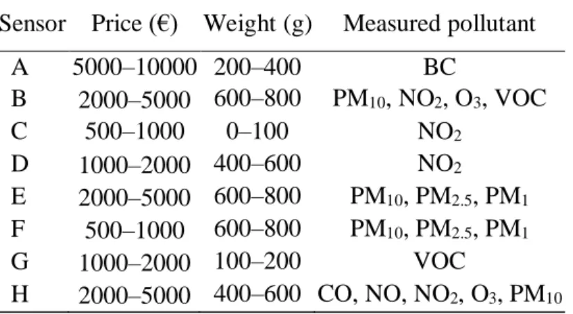
Eight sensors were tested during the selection tests. The main specifications are listed in 209
Table 2. 210
3.1 Static ambient air tests
For static ambient air tests the results of six of them are presented (the sensors G and F showed 212
aberrant values). An example of the time series is given for the sensors A, B and C in Fig. 2 and 213
gives a preliminary assessment of the sensors’ reliability. As shown in Fig. 2, the results from 214
several days of continuous measurements of sensors versus reference instruments are 215
heterogeneous among the different sensors and thus difficult to assess. The first time series 216
exhibits a BC sensor (black line), which gave results very close to the reference instrument (grey 217
line). For this sensor, the results were satisfying: the two lines are almost always overlapping. 218
This first basic tool (studying the time series) identified sensor A as being in agreement with the 219
project expectations. 220
However, the results were not always that unambiguous, and some sensors gave medium 221
results like the nitrogen dioxide sensors presented in the second time series (Fig. 2). For these two 222
devices, it is difficult to assess the performance of the sensors by only using the time series. 223
Furthermore, the difference with the reference instrument and the correlation are not the only 224
characteristics to focus on, but also the medium term shifting, the lack of data, dynamics, etc. are 225
important. This is why the SET tool (presented in the methods section) is relevant. 226
In Table 3, the integrated performance index (IPI) and the other SET results are presented for 227
the six sensors used in this work. The measurements time bases and the dates of the considered 228
period of time are also given here. BC measurements were done only by sensor A. The satisfying 229
performance of this sensor demonstrated with the time series is corroborated by the SET 230
evaluation, with a very good IPI of 0.91, which is due to the high results for every single 231
parameter. Ozone was only measured by sensor B. For this pollutant, the IPI is mediocre with a 232
value of 0.46. This is explained by the non-negligible data loss: the presence is 0.75, which 233
means that one value out of four is missing. Furthermore, the RMSE is high (15 ppb) compared 234
with the mean value of 8 ppb, and even the match score (0.3) is poor. Three sensors measured 235
NO2. The best one was sensor B, with an IPI of 0.76 and a RMSE of 5 ppb. Sensor C gave poor 236
results and even aberrant values highlighted by very low correlation coefficients (below 0.15). 237
Sensor D has a fair correlation coefficient (higher than 0.5) but suffers from a large RMSE 238
(37 ppb), poor match score (0.24) and quite significant data loss (presence of 67 %). Particulate 239
matter was measured by three sensors: sensor B measured PM10 and the sensors E and F 240
measured PM10, PM2.5 and PM1. Sensor F gave the best results for all the PM sizes, with an IPI of 241
0.64, 0.80 and 0.78 for PM10, PM2.5 and PM1, respectively. The others gave a much lower IPI. 242
The major advantage of sensor F is the data availability, which does not suffer from data loss. Its 243
match score is acceptable for the three PM sizes (always larger than 0.6) although this parameter 244
is lower than 0.43 for the others. Even if its RMSE is large, sensor F gives a relevant 245
approximation of the PM concentration. 246
This first static ambient test led us to rule out sensor E, which gave aberrant values for PM10, 247
as well as sensor D because of its non-satisfactory results. Sensor B was kept despite the 248
mediocre results for O3 (IPI of 0.46) and PM10 (IPI of 0.40), thanks to its multi-pollutant 249
measuring ability and because the producing firm should improve the sensor before the next 250
testing step. Sensor C gave here poor results, but the authors were aware that good results had 251
been obtained with this device, and it was suggested that these unsatisfactory results could be due 252
to an out-of-date electrochemical sensing cell or an inappropriate storage, which would lower the 253
sensor performance. This is why new units of this sensor were purchased for the following testing 254
steps. 255
3.2 Mobility/reproducibility test
256
This test involved the following sensors: sensor B, sensor C and sensor F. The BC sensor A 257
was not involved in this mobility tests because studies (Ezani et al., 2018; Lin et al., 2017) have 258
already demonstrated its ability to perform mobile measurements. Fig. 3 and Fig. 4 (and Fig. S1 259
in Appendix) show, for the three units of each sensor, the entire time series for every sensor of 260
each pollutant and the comparison with the Airparif stations when the route goes by these stations. 261
Fig. 3 refers to the NO2 sensors. The whole-day time series shows that sensors C present a better 262
reproducibility between the units than sensors B. Secondly, the sensors C show a better dynamic 263
response whereas sensors B present averaged values. Moreover, this figure demonstrates the 264
sensitivity of the sensors C to monitor the environmental changes. Three specific environments 265
are pointed out in the time series: “Opéra” is an Airparif monitoring station classified as traffic 266
influenced, “Restaurant” refers to the lunch break, which took place in a cafeteria and “Bus” 267
stands for bus travel. Sensor C was able to identify different levels associated with different 268
environments: NO2 was high (around 50 ppb) during the time spent close to the Opéra traffic 269
location, low (about 10 ppb) in the restaurant (indoors) and presented strong variations during bus 270
travel. Furthermore, these sensors quickly detected the environment changes. On the contrary, 271
sensors B were very slow to monitor pollutant level variations, and were unable to properly 272
discriminate environmental changes. Below the main time series, graphs allow us to estimate the 273
accuracy of the sensors against Airparif stations, which can be considered as reference 274
measurements. Except for the “Paris centre” station, the three sensors C were in the right range; 275
the variations were also well monitored, especially for the “Célestins” and “Opéra” stations. The 276
sensors B never showed clear variation, and a significant difference existed between the three 277
units (up to tens of ppb for the “RN2” station). Fig. 4 shows the mobility test results for PM10 278
sensors B and F. The time series depict poor consistency between the units, especially for sensor 279
B, for which a gap of up to 50 µg m–3 was observed. The comparison with the Airparif stations 280
shows that sensors B gave poor results: for the stations “Paris centre” and “Bobigny”, the sensor 281
values were significantly different from the reference; for the “Opéra” station, results were fair (a 282
shift of about 10 µg m–3 appears); and for the “RN2” station, the difference between the three 283
units was substantial (about 30 µg m–3). Results were better for the sensors F: the sensors were 284
almost always in the range of the reference station, with an inter-sensor difference not larger than 285
20 µg m–3. Nevertheless, sensors F results were poor for the “Bobigny” station, for which the 286
difference with the reference went up to 30 µg m–3.Three units of each sensor (B, C and F) were 287
tested during this mobility steps. Sensors C and F presented the best results. 288
3.3 Selected sensors
289
The BC sensor A gave satisfying results and was therefore selected for the next step. The 290
sensors C gave suitable results during the mobility tests, which confirms the hypothesis that a 291
deteriorated unit was used during the static measurement tests. This sensor gave better results 292
than sensor B for NO2. The PM sensor F gave more accurate results than sensor B. For this 293
reason and because of the poor results for NO2 and O3, sensor B was excluded. 294
The retained sensors were sensors A (BC), C (NO2) and F (PM10, PM2.5 and PM1). The next 295
section deals with the assessment of their capabilities. Several units of each of the three sensors 296
were purchased: 15 units for the sensors C and F, and 6 units for the sensor A (due to its high 297
cost). 298
3.4 Reproducibility tests in static measurements
299
An overview of the results is presented in Fig. 5. From the top to the bottom, are presented the 300
BC, NO2 and PM2.5 measurements. The reference instrument is plotted in black and the sensors in 301
coloured lines. Generally, the sensors closely followed the reference instrument trend even if 302
some discrepancies were observed. The BC sensors A were very accurate, despite some noisy 303
periods. On the whole, the NO2 sensors C overestimated the concentration, this is certainly due to 304
the low NO2 ambient concentration compared with the limit of detection (20 ppb according to the 305
manufacturer’s specifications). This behaviour was already observed by Duvall et al. (2016). 306
Even if these sensors were still able to monitor the global variability in these conditions, another 307
measurement campaign was conducted. The objective was to submit the sensors to NO2 ambient 308
levels higher than the devices’ detection limit. From August 28th to September 4th, fifteen NO2 309
sensors C were used to measure conditions at the Airparif station close to a major road (Paris ring 310
road). The results overview is presented in Appendix (Fig. S2), the rest of this work is based on 311
the results from this experiment. Concerning the PM sensors F, they were both quite close to the 312
reference and very reproducible to one another, except for one unit plotted in light green, which 313
presented erratic values. For the PM2.5, the mean RMSE is 6 µg m–3, which is fairly low 314
compared with the measured concentration in mobility in Paris and its suburbs (often higher than 315
40 µg m–3). 316
The SET results for the BC sensors are presented in details in Table S2 in appendix. The IPI is 317
high (around 0.8) for all the sensor units. These sensors did not suffer from data loss at all (the 318
presence parameter is always almost 100 %). The reproducibility between the units can be 319
quantified by the measuring range, defined as the average of the difference across the units 320
between the maximum and the minimum for each measurement date. For these BC sensor units, 321
the measurement range is 616 ng m–3, which is not negligible but below the mean concentration 322
value. 323
The SET results for the fifteen NO2 sensor units (Table S3 in appendix) are homogeneous, the 324
IPI spans from 0.75 to 0.79. The mean measured concentration was above 40 ppb, which is 325
higher than the limit of detection. This leads to good correlation coefficients (above 0.76 for the 326
mean Pearson coefficient) and reasonable RMSE compared with the ambient levels (mean RMSE 327
is 14 ppb). Moreover, data loss was very uncommon as shown by the presence parameter. 328
The PM SET results are presented in Tables S4, S5 and S6 in appendix for the three PM sizes. 329
Regarding PM2.5 sensor units, the IPI is above 0.68, except for the sensor unit F7, which was 330
defective (plotted in light blue in Fig. 5). The presence is higher than 0.72 (except for F6 at 0.62): 331
the sensor units F data loss was low. The correlation coefficients were never below 0.6, which 332
shows good agreement with the reference. The mean measuring ranges for the three classes of 333
PM are 16 µg m–3, 19 µg m–3 and 20 µg m–3 for PM1, PM2.5 and PM10, respectively. These 334
measuring ranges are not negligible but the mean RMSE values are lower: 4 µg m–3, 6 µg m–3 335
and 14 µg m–3 for PM1, PM2.5 and PM10, respectively. This means that a discrepancy existed 336
between the units, but the general agreement with the true value is acceptable. 337
3.5 Chamber controlled test
338
Fig. 6 shows the results of this test. The top chart represents the controlled parameters 339
monitored: humidity and NO2 concentration. The three others are the sensors results. 340
The sensor F values were always zero: it was not affected at all by humidity changes (at least 341
in the absence of PM). The BC sensor A was clearly affected by humidity variations as it showed 342
BC concentration variations at the same time as humidity ones. When the humidity was 343
decreasing, a positive artefact of up to 250 ng m–3 was observed. Conversely, a negative artefact 344
of 150 ng m–3 was reached when the humidity decreased to 40 % RH. The mean value and the 345
standard deviation of this sensor over the constant humidity period were respectively 15 ng m–3 346
and 14 ng m–3, which is low compared with ambient levels. Two NO2 sensor units C were 347
measuring in the chamber. They presented a sensitivity to humidity changes with the same 348
pattern as the BC sensor. The positive artefacts went up to 66 ppb and the negative artefact was 349
constrained at zero (there is no negative value). We have also to note that the two sensor units 350
gave results close to one another, with a RMSE of 7 ppb. Over constant humidity and a NO2 351
concentration of 25 ppb, their mean values were 21 ppb and 26 ppb with a standard deviation 352
around 1 ppb. 353
The second test conducted in the controlled chamber was the NO2 variation (Fig. S3 in 354
Appendix). This experiment consisted of a succession of one-hour steps of 0 ppb, 50 ppb, 355
100 ppb, 200 ppb, 0 ppb and a final longer 50 ppb stage over several hours. Inside the chamber, 356
the relative humidity was set at 60 % and there is no particulate matter. 357
The ability of the sensors to monitor quick concentration changes was demonstrated here as the 358
two sensor units reacted at the same time as the reference instrument. The sensor units were able 359
to monitor increases (up to 200 ppb) and decreases down to 0 ppb. However, a gap can be 360
observed between the sensor units and the reference, the associated RMSE is 11 ppb and 15 ppb. 361
For the final longer step at 50 ppb, the RMSE stood at 9 ppb and 2 ppb. 362
To conclude for the controlled chamber tests, although sensor F presented no artefacts due to 363
humidity changes (with a zero concentration of PM), the sensors A and C were sensitive to 364
humidity. During the following campaigns, this will have to be taken into account, a correction or 365
an invalidation protocol may be needed. 366
3.6 Feasibility campaign
367
The feasibility campaign was conducted with fifteen volunteers from Monday 18th to Friday 368
22nd June 2018. One sensor unit C and one sensor unit F were given to each volunteer and six 369
sensor units A were shared between the participants. This campaign was conceived as a proof of 370
the Polluscope concept, thus, only a limited analysis of the results was done. 371
Globally, the campaign was a success: all the sensor units were worn for the whole week. The 372
data availability (the time resolution was one minute) is 66 % for sensors A and 69 % for sensors 373
F, which can be considered as a satisfying result. The data loss was due to minor problems and 374
routine maintenance (filter change, turning on and off, powering, etc.). However, the data 375
availability for the sensors C only reaches 41 %. This was caused by storage memory erasure 376
when the sensor ran out of power. The coming campaigns protocols will prevent this issue. 377
Generally, the data availability was slightly lower than during the previous tests, this was due to 378
the campaign environment and the fact that the sensor units were operated by volunteers without 379
expert skills. 380
Fig. 7 shows the results of the three sensor units worn for the whole week by a volunteer. Four 381
kinds of environments are pointed out: “indoor” for the time spent inside, “polluted indoor” for 382
emitting activities conducted indoors (cafeteria, smoking or cooking, for instance), “commuting” 383
journeys (whatever the travel mode) and “outdoor” for the time spent outside any building. The 384
indoor environment is the more frequent environment, nevertheless, the spikes were usually 385
observed during commuting or in polluted indoor environments. The major BC and NO2 peaks 386
occurred most frequently during commuting trips. Inversely, the highest particulate values were 387
measured during “polluted indoor” episodes. An example of contrasted environments 388
(commuting, indoors and tobacco smoke in indoor environment) measurements is presented in 389
Appendix, Fig. S4. During the campaign, artefacts due to quick environmental change (studied in 390
the controlled chamber in Section 3.5) were observed; this is more detailed in Appendix, Fig. S5). 391
This feasibility campaign demonstrated the capability of the Polluscope protocol to conduct a 392
campaign lasting a whole week with volunteers. The results from the sensors enable us to 393
discriminate several emitting activities; a preliminary estimation of the personal exposure is thus 394
available. 395
4 DISCUSSION
396
The first stages of Polluscope (the selection and assessment of the sensors) have been 397
conducted. The AE51 (BC), the Cairclip (NO2) and the Canarin (PM10, PM2.5 and PM1) have 398
been selected and assessed. The feasibility campaign demonstrated that these three sensors are 399
reliable enough to be used for full-scale campaigns involving volunteers from the general public. 400
Their ability to discriminate different environments (commuting trips, polluted or clean indoor 401
environment, etc.) has been proven. 402
For the static measurement assessments, we used the SET algorithm designed by Fishbain et al. 403
(2017), available as an open source resource4. In their article, they presented results from 25 404
AQMesh NO2 sensor units that had taken measurements for about three months in static positions. 405
The mean related IPI is 0.58, this is very close to our mean Cairclip IPI (from the reproducibility 406
test) of 0.54; even if the Cairclip is designed for mobile measurements whereas the AQMesh 407
system is designed for static monitoring (i.e. expecting to have a better performance than a 408
portable device). Knowing the successful deployment of the AQMesh sensor units, this result 409
demonstrates the reliability of the Cairclip. Fishbain et al. (2017) also used the SET with PM 410
sensors (DC1700 Dylos and GeoTech), the mean resulting IPI is 0.63. The PM2.5 Canarin sensor 411
used in our study gave significantly better results with a mean IPI of 0.73. 412
The SET algorithm was also used by Broday and the Citi-Sense Project Collaborators (2017). 413
They presented unpublished results from about three months of ambient air measurements of six 414
PM10 sensor units located in Ostrava, Czech Republic. The mean IPI is 0.72, which is very close 415
to the result from our study (0.73). 416
Due to its recent release, SET algorithm results have not been published in other articles yet. 417
To the best of our knowledge, our study is the first to apply the SET evaluation to the AE51 and 418
the Cairclip sensors. However, these two devices have been largely used and several results have 419
been published, some of the more relevant for our study are discussed below. 420
4.1 Static comparison
421
Lin et al. (2017) compared AE51 with reference instruments and found a good mean 422
correlation of 0.77. Viana et al. (2015) conducted a study involving six AE51 and a reference 423
station in static measurements, the correlation coefficient was above 0.75. In our study, the mean 424
correlation coefficient was 0.80. This higher agreement may be due to higher inlet flow 425
(150 mL min–1 compared with 100 mL min–1 in the Viana et al. (2015) study) or coarser time 426
resolution (1 min in our study and 1 sec in the Lin et al. (2017) study). 427
Several other studies have pointed to the good results of this black carbon sensor in agreement 428
with our results (Cai et al., 2014; Gillespie et al., 2017; Velasco and Tan, 2016). 429
The recent low-cost sensors review by the World Metrological Organization (Lewis et al., 430
2018) described several performance evaluation programs as the work supported by the United 431
States Environment Protection Agency (EPA)5; they described an air sensor toolbox where the 432
main performances of tens of sensors were gathered and compared. For the Cairclip NO2 sensor, 433
the EPA and Jiao et al. (2016) state that a correlation coefficient between 0.42 and 0.76 was 434
obtained with reference instruments. Our mean Pearson correlation was 0.76, which is in the high 435
part of the EPA range. The additional information given by the SET algorithm in our study is the 436
good match score of 0.64 and the absence of data loss (the presence parameter reaches almost 437
100 %). Another example is the study conducted by Spinelle et al. (2015). They found a 438
correlation of up to 0.75 for the Cairclip sensor units. This result is both in the EPA range and 439
close to our result of 0.76. 440
Due to its new release, only a few research works including Canarin have been conducted. For 441
instance, Tse et al., 2018B presented a project based on static measurements from four Canarin 442
units. Some tests were conducted in Bologna, Italia, and PM10 maps have been produced. These 443
works were preliminary and the most accomplished article about Canarin sensor is certainly the 444
one conducted by Tse et al., 2018A. They deployed nine Canarin units in a library inducted at the 445
UNESCO world heritage list. The sensors were measuring 24/7 for months (from Summer 2017 446
to Spring 2018), which enabled to show that a clear diurnal pattern occurred with higher levels 447
during night time. On a longer period of time it was the winter season which experienced more 448
pollution. This protocol also permitted to quantify that 56 % of the time, the PM2.5 air pollution 449
level was low according to the EPA standards (below 12 µg m-3). The coming improvements 450
announced in these three articles suggested a wider use of the Canarin in a near future. Overall, 451
these works underlined the promising capabilities of this sensor. The present paper confirmed this 452
first evaluation and went a step further (larger amount of units, mobile measurements, etc.) to 453
prove the ability to use the Canarin to equip volunteers for the personal exposure quantification. 454
4.2 Mobile measurements
455
It is usually more difficult to robustly assess sensor accuracy in mobile measurements as the 456
reference instruments are unlikely to be usable in motion. A metric that can be used is the 457
agreement between several units of portable sensors (previously assessed – or not – in static 458
measurements versus a reference instrument). This provides information on the reproducibility 459
and thus on the reliability of the mobile device. Another possibility is to compare the sensor 460
measurements with static stations considered as a reference if the mobility route goes close to this 461
kind of monitoring site. 462
The Ezani et al. (2018) study was based on mobile measurements performed with two AE51 463
units. There were no reference instruments but the correlation between the two units was good: 464
0.92. Lin et al. (2017) performed mobile AE51 measurements. Comparison was possible thanks 465
to 17 transient immobile periods (of less than one hour) nearby reference stations. The AE51 unit 466
showed an interquartile range agreement with the reference instrument of 82 %. High-resolution 467
mapping is possible with the AE51, as in the study of den Bossche et al. (2015) where sensor 468
units were mounted on bikes in Antwerp, Belgium. A 50-meter resolution was obtained with an 469
uncertainty of 25 %. Pant et al. (2017) performed a study aiming at quantifying personal 470
exposure to BC in New Delhi, India. The AE51 were given to volunteers and environments 471
(commuting, cooking, etc.) were distinguished. 472
Few studies have been published on the Cairclip sensor being used in mobile measurements, 473
especially compared with the abundant literature related to the AE51. The recent work by 474
Chambers et al. (2018) found no consistent relationship between NO2 concentrations and health 475
parameters. The authors state that the Cairclip was able to appropriately monitor personal 476
exposure and a clear diurnal cycle was observed but no more validation data was provided. The 477
study by Reid (2015) is based on the qualification of Cairclip sensors. Mobile measurements 478
were conducted with two Cairclip units in different environments: public transport, outdoor and 479
indoor. The sensors monitored interesting variability, especially close to traffic. 480
Lastly, Aguiari et al., 2018 introduced a possible use of the Canarin by attaching them to bikes. 481
4.3 Methodology discussion
482
Our work has revealed that the three selected sensors are appropriate for personal exposure 483
assessment. Beyond that first result, the Polluscope selection and assessment methodology was 484
also an outcome of this study. 485
It is now well known, even in the emerging field of small air quality sensors that a complete 486
sensor assessment is of primary importance to obtain reliable data. Some studies were only based 487
on laboratory experiments (Manikonda et al., 2016; Ng et al., 2018), but in-the-field calibration 488
was identified as necessary to properly assess the sensors’ capabilities (Castell et al., 2017; 489
Schneider et al., 2017) as the results can be substantially different from laboratory-controlled 490
environments. For instance, during our tests, the Cairclip showed better results during the 491
controlled chamber tests. The ambient air tests were very useful to reveal that the Cairclip had 492
difficulties in measuring low ambient concentrations. 493
As seen in the section concerning the reproducibility tests, non-negligible differences were 494
observed between units of the same sensor. This highlights the importance of testing several units 495
at a time. In this study, we conducted tests with 6 AE51, 15 Cairclip and 15 Canarin. For some of 496
the previously published studies, the small number of tested units was a limitation, for example, 497
Lin et al. (2017) (two AE51 and only one for the mobility tests), Ezani et al. (2018) (two AE51), 498
Duvall et al. (2016) (two Cairclip). 499
4.4 Conclusions
500
No remote sensor is perfect, and the three selected ones are the result of compromises and each 501
have strengths and weaknesses. The AE51 is accurate, its IPI (above 0.8) is higher than all other 502
sensors. This BC sensor is also reliable and easy to use with very little data loss. But it is 503
sensitive to humidity, which leads to some artefacts when quick environmental changes occur, 504
and its high price is also a weakness because fewer units can be purchased. The Cairclip is very 505
light and thus easy to carry all day long, but the storage memory is erased if the sensor unit runs 506
out of battery, thus it is consequently more demanding for the operator. Moreover, even if these 507
sensors demonstrated their ability to perform reliable measurements in mobile measurement (see 508
related section), the detection limit (20 ppb) is not appropriate for low NO2 levels. The Canarin is 509
able to send data via Wi-Fi and has a high storage capacity (several weeks of measurements), 510
which is useful when the data sending is not possible. Its robustness in mobility is also an 511
important advantage: the Canarin was the sensor that presented the highest data availability 512
during the feasibility campaign (69 %). This sensor showed satisfying results for the PM2.5 513
measurements (IPI of 0.7) but substantially lower for PM10 (IPI of 0.4). Finally, the weight of the 514
sensor unit (it is quite heavy) is a drawback. 515
Even if the three selected sensors have some weaknesses, their ability to be used in mobile 516
measurements has been demonstrated. For the coming campaigns, attention will be given to their 517
drawbacks. 518
To conclude, the Polluscope project is one of the few studies that has conducted an in-depth 519
sensor assessment including the most important following steps: 520
Several kinds of tests were performed. Ambient air static measurement tests against 521
reference instruments was the first assessment of the sensors in real atmosphere with 522
natural meteorological parameters variability (temperature, humidity, wind speed and 523
direction, etc.) The laboratory tests were of primary importance to quantify the sensors; 524
responses to rapid atmospheric changes (i.e., humidity, pollutants levels). Mobile 525
measurements were necessary as the project goal is to use the sensors for personal 526
exposure, to be worn by volunteers. 527
A large number of units of each sensor was tested to quantify the reproducibility and to 528
eliminate problems arising from a single deficient unit. 529
A robust multi-metric static measurement assessment with the SET algorithm was 530
conducted in order to be as rigorous as possible in the assessment. 531
The next stage of the Polluscope project will be the full-scale campaigns involving fifteen 532
volunteers each week during the six weeks per studied season. These campaigns will take place 533
over two years and will involve 160 people. Even if the size of the project is already consistent, a 534
valuable perspective would be to recruit more volunteers over a larger area in order to increase 535
the representativeness of the study. 536
538
ACKNOWLEDGEMENTS
539
This project was funded by the French agency: Agence nationale de la recherche (ANR – 540
http://www.agencenationale-recherche.fr/Projet-ANR-15-CE22-0018). Part of the equipment was
541
funded by iDEX Paris-Saclay, in the framework of the project ACE-ICSEN. Measurements from 542
the SIRTA station were performed within the ACTRIS research infrastructure under the H2020 543
grant agreement 654109. Additional support from CEA and CNRS are acknowledged. 544
546
REFERENCES
547
Adgate, J.L., Church, T.R., Ryan, A.D., Ramachandran, G., Fredrickson, A.L., Stock, T.H., 548
Morandi, M.T. and Sexton, K. (2004). Outdoor, indoor, and personal exposure to VOCs in 549
children. Environ. Health Perspect. 112(14): 1386–1392. 550
Aguiari, D., Delnevo, G., Monti, L., Ghini, V., Mirri, S., Salomoni, P., Pau, G., Im, M., Tse, R., 551
Ekpanyapong, M., and Battistini, R. (2018). Canarin ii : Designing a smart e-bike eco-system. 552
15th IEEE Annual Consumer Communications & Networking Conference (CCNC) 1-6
553
Airparif – La qualité de l'air dans les enceintes du métro ou du rer, 554
https://www.airparif.asso.fr/pollution/air-interieur-metro, Accessed: 22 November 2018.
555
Airparif (2017). Bilan de la qualité de l'air 2016 – surveillance et information en Île-de-France. 556
Airparif (2018). Bilan de la qualité de l'air 2017 – surveillance et information en Île-de-France. 557
Airparif (2019). Bilan de la qualité de l'air 2018 – surveillance et information en Île-de-France. 558
Borghi, F., Spinazzè, A., Rovelli, S., Campagnolo, D., Del Buono, L., Cattaneo, A., and Cavallo, 559
D.M. (2017). Miniaturized monitors for assessment of exposure to air pollutants: A review. Int. 560
J. Environ. Res. Public Health 14(8): 909.
561
den Bossche, J.V., Peters, J., Verwaeren, J., Botteldooren, D., Theunis, J. and Baets, B.D. (2015). 562
Mobile monitoring for mapping spatial variation in urban air quality: Development and 563
validation of a methodology based on an extensive dataset. Atmos. Environ. 105: 148–161. 564
Broday, D.M. and the Citi-Sense Project Collaborators (2017). Wireless distributed 565
environmental sensor networks for air pollution measurement: the promise and the current 566
reality. Sensors 17(10): 2263. 567
Burkart, J., Steiner, G., Reischl, G., Moshammer, H., Neuberger, M. and Hitzenberger, R. (2010). 568
Characterizing the performance of two optical particle counters (grimm opc1.108 and opc1.109) 569
under urban aerosol conditions. J. Aerosol Sci. 41(10): 953–962. 570
Cai, J., Yan, B., Ross, J.M., Zhang, D., Kinney, P.L., Perzanowski, M.S., Jung, K., Miller, R.L. 571
and Chillrud, S.N. (2014). Validation of microaeth® as a black carbon monitor for fixed-site 572
measurement and optimization for personal exposure characterization. Aerosol Air Qual. Res. 573
14(1): 1–9. 574
Castell, N., Dauge, F.R., Schneider, P., Vogt, M., Lerner, U., Fishbain, B., Broday, D. and 575
Bartonova, A. (2017). Can commercial low-cost sensor platforms contribute to air quality 576
monitoring and exposure estimates? Environ. Int. 99: 293–302. 577
Castell, N., Kobernus, M., Liu, H.-Y., Schneider, P., Lahoz, W., Berre, A.J. and Noll, J. (2015). 578
Mobile technologies and services for environmental monitoring: The Citi-sense-MOB 579
approach. Urban Clim. 14(Part 3): 370–382. 580
Chambers, L., Finch, J., Edwards, K., Jeanjean, A., Leigh, R. and Gonem, S. (2018). Effects of 581
personal air pollution exposure on asthma symptoms, lung function and airway inflammation. 582
Clin. Exp. Allergy, 48(7): 798–805.
583
Deville Cavellin, L., Weichenthal, S., Tack, R., Ragettli, M.S., Smargiassi, A. and Hatzopoulou, 584
M. (2016). Investigating the use of portable air pollution sensors to capture the spatial 585
variability of traffic-related air pollution. Environ. Sci. Technol. 50(1): 313–320. 586
Duvall, R.M., Long, R.W., Beaver, M.R., Kronmiller, K.G., Wheeler, M.L. and Szykman, J.J. 587
(2016). Performance evaluation and community application of low-cost sensors for ozone and 588
nitrogen dioxide. Sensors 16(10): 1698. 589
European Environment Agency (2017). Air quality in Europe 2017 report. European 590
Environment Agency. 591
Ezani, E., Masey, N., Gillespie, J., Beattie, T.K., Shipton, Z.K. and Beverland, I.J. (2018). 592
Measurement of diesel combustion-related air pollution downwind of an experimental 593
unconventional natural gas operations site. Atmos. Environ. 189: 30–40. 594
Fishbain, B., Lerner, U., Castell, N., Cole-Hunter, T., Popoola, O., Broday, D.M., Iñiguez, T.M., 595
Nieuwenhuijsen, M., Jovasevic-Stojanovic, M., Topalovic, D., Jones, R.L., Galea, K.S., Etzion, 596
Y., Kizel, F., Golumbic, Y.N., Baram-Tsabari, A., Yacobi, T., Drahler, D., Robinson, J.A., 597
Kocman, D., Horvat, M., Svecova, V., Arpaci, A. and Bartonova, A. (2017). An evaluation 598
tool kit of air quality micro-sensing units. Sci. Total Environ. 575: 639–648. 599
Gao, M., Cao, J. and Seto, E. (2015). A distributed network of low-cost continuous reading 600
sensors to measure spatiotemporal variations of PM2.5 in Xi'an, China. Environ. Pollut. 199: 601
56–65. 602
Gillespie, J., Masey, N., Heal, M.R., Hamilton, S. and Beverland, I.J. (2017). Estimation of 603
spatial patterns of urban air pollution over a four-week period from repeated 5-min 604
measurements. Atmos. Environ. 150: 295–302. 605
Hasenfratz, D., Saukh, O., Walser, C., Hueglin, C., Fierz, M., Arn, T., Beutel, J. and Thiele, L. 606
(2015). Deriving high-resolution urban air pollution maps using mobile sensor nodes. 607
Pervasive Mob. Comput. 16(Part B): 268–285.
608
Hinds, W.C. and Bellin, P. (1988). Effect of facial-seal leaks on protection provided by half-mask 609
respirator. Appl. Ind. Hyg. 3(5): 158–164. 610
Holstius, D.M., Pillarisetti, A., Smith, K.R. and Seto, E. (2014). Field calibrations of a low-cost 611
aerosol sensor at a regulatory monitoring site in California. Atmos. Meas. Tech. 7(4): 1121– 612
1131. 613
Hu, K., Sivaraman, V., Luxan, B.G. and Rahman, A. (2016). Design and evaluation of a 614
metropolitan air pollution sensing system. IEEE Sens. J. 16(5): 1448–1459. 615
Hu, K., Wang, Y., Rahman, A. and Sivaraman, V. (2014). Personalising pollution exposure 616
estimates using wearable activity sensors. In 2014 IEEE Ninth International Conference on 617
Intelligent Sensors, Sensor Networks and Information Processing (ISSNIP) (pp. 1–6).
618
IARC (2013). Air pollution and cancer. IARC Scientific Publications. 619
Janssen, N.A., Hoek, G., Simic-Lawson, M., Fischer, P., van Bree, L., ten Brink, H., Keuken, M., 620
Atkinson, R.W., Anderson, H.R., Brunekreef, B. and Cassee, F.R. (2011). Black carbon as an 621
additional indicator of the adverse health effects of airborne particles compared with PM10 and 622
PM2.5. Environ. Health Perspect. 119(12): 1691–1699. 623
Jarjour, S., Jerrett, M., Westerdahl, D., de Nazelle, A., Hanning, C., Daly, L., Lipsitt, J. and 624
Balmes, J. (2013). Cyclist route choice, traffic-related air pollution, and lung function: a 625
scripted exposure study. Environmental Health 12(1): 14. 626
Jiao, W., Hagler, G., Williams, R., Sharpe, R., Brown, R., Garver, D., Judge, R., Caudill, M., 627
Rickard, J., Davis, M., Weinstock, L., Zimmer-Dauphinee, S. and Buckley, K. (2016). 628
Community air sensor network (Cairsense) project: evaluation of low-cost sensor performance 629
in a suburban environment in the south-eastern United States. Atmos. Meas. Tech. 9(11): 5281– 630
5292. 631
Klepeis, N.E., Nelson, W.C., Ott, W.R., Robinson, J.P., Tsang, A.M., Switzer, P., Behar, J.V., 632
Hern, S.C. and Engelmann, W.H. (2001). The national human activity pattern survey (NHAPS): 633
A resource for assessing exposure to environmental pollutants. J. Exposure Anal. Environ. 634
Epidemiol. 11(3): 231–252.
635
Lewis, A.C., von Schneidemesser, E. and Peltier, R.E. (2018). Low-cost sensors for the 636
measurement of atmospheric composition: overview of topic and future applications. World 637
Meteorological Organization, 1215.
638
Lin, C., Gillespie, J., Schuder, M., Duberstein, W., Beverland, I. and Heal, M. (2015). Evaluation 639
and calibration of aeroqual series 500 portable gas sensors for accurate measurement of 640
ambient ozone and nitrogen dioxide. Atmos. Environ. 100: 111–116. 641
Lin, C., Masey, N., Wu, H., Jackson, M., Carruthers, D.J., Reis, S., Doherty, R.M., Beverland, I.J. 642
and Heal, M.R. (2017). Practical field calibration of portable monitors for mobile 643
measurements of multiple air pollutants. Atmosphere 8(12): 231. 644
Liu, J.C. and Peng, R.D. (2018). Health effect of mixtures of ozone, nitrogen dioxide, and fine 645
particulates in 85 US counties. Air Qual. Atmos. Health. 11(3): 311–332. 646
Manikonda, A., Zikova, N., Hopke, P.K. and Ferro, A.R. (2016). Laboratory assessment of low-647
cost PM monitors. J. Aerosol Sci. 102: 29–40. 648
Mead, M., Popoola, O., Stewart, G., Landsho, P., Calleja, M., Hayes, M., Baldovi, J., McLeod, 649
M., Hodgson, T., Dicks, J., Lewis, A., Cohen, J., Baron, R., Saffell, J. and Jones, R. (2013). 650
The use of electrochemical sensors for monitoring urban air quality in low-cost, high-density 651
networks. Atmos. Environ. 70: 186–203. 652
Ng, C.-L., Kai, F.-M., Tee, M.-H., Tan, N. and Hemond, H.F. (2018). A prototype sensor for in 653
situ sensing of fine particulate matter and volatile organic compounds. Sensors 18(1): 265. 654
Niranjan, R. and Thakur, A.K. (2017). The toxicological mechanisms of environmental soot 655
(black carbon) and carbon black: focus on oxidative stress and inflammatory pathways. Front. 656
Immunol. 8: 763.
657
Pant, P., Habib, G., Marshall, J.D. and Peltier, R.E. (2017). PM2.5 exposure in highly polluted 658
cities: a case study from New Delhi, India. Environ. Res. 156: 167–174. 659
Peng, I.H., Chu, Y.Y., Kong, C.Y. and Su, Y.S. (2013). Implementation of indoor VOC air 660
pollution monitoring system with sensor network. In 2013 Seventh International Conference 661
on Complex, Intelligent, and Software Intensive Systems (pp. 639–643).
662
Reid, B. (2015). A quantitative analysis of the Cairclip O3/NO2 sensor. Thesis, University of 663
Alberta. 664
Sante Publique France (2016). Impacts sanitaires de la pollution de l'air en France : nouvelles 665
données et perspectives. Sante Publique France. 666
Schneider, P., Castell, N., Vogt, M., Dauge, F.R., Lahoz, W.A. and Bartonova, A. (2017). 667
Mapping urban air quality in near real-time using observations from low-cost sensors and 668
model information. Environ. Int. 106: 234–247. 669
Schwartz, J., Dockery, D.W. and Neas, L.M. (1996). Is daily mortality associated specifically 670
with fine particles? J. Air Waste Manage. Assoc. 46(10): 927–939. 671
Sousan, S., Koehler, K., Thomas, G., Park, J.H., Hillman, M., Halterman, A. and Peters, T.M. 672
(2016). Inter-comparison of low-cost sensors for measuring the mass concentration of 673
occupational aerosols. Aerosol Sci. Technol. 50(5): 462–473. 674
Spinelle, L., Gerboles, M., Kok, G., Persijn, S. and Sauerwald, T. (2017). Review of portable and 675
low-cost sensors for the ambient air monitoring of benzene and other volatile organic 676
compounds. Sensors 17(7): 1520. 677
Tse, R., Aguiari, D., Chou, K.S., Tang, S.K., Giusto, D., and Pau, G. (2018A) Monitoring cultural 678
heritage buildings via low-cost edge computing/sensing platforms: The biblioteca joanina de 679
coimbra case study. 4th International Conference on Smart Objects and Technologies for 680
Social Good, Goodtechs 148-152.
681
Tse, R., Monti, L., Prandi, C., Aguiari, D., Pau, G., and Salomoni, P. On assessing the accuracy 682
of air pollution models exploiting a strategic sensors deployment (2018B). 4th EAI 683
International Conference on Smart Objects and Technologies for Social Good, Goodtechs
55-684
58. 685
Velasco, A., Ferrero, R., Gandino, F., Montrucchio, B. and Rebaudengo, M. (2016). A mobile 686
and low-cost system for environmental monitoring: a case study. Sensors 16: 710. 687
Velasco, E. and Tan, S.H. (2016). Particles exposure while sitting at bus stops of hot and humid 688
Singapore. Atmos. Environ. 142: 251–263. 689
Viana, M., Rivas, I., Reche, C., Fonseca, A., Perez, N., Querol, X., Alastuey, A., Alvarez 690
Pedrerol, M. and Sunyer, J. (2015). Field comparison of portable and stationary instruments for 691
outdoor urban air exposure assessments. Atmos. Environ. 123(Part A): 220–228. 692
World Health Organization (2014). Seven million premature deaths annually linked to air 693
pollution. http://www.who.int/mediacentre/news/releases/2014/air-pollution/en/. Accessed: 22 694
November 2018. 695
World Health Organization (2012). Health effects of black carbon. World Health Organization. 696
World Health Organization (2003). Health aspects of air pollution with particulate matter, ozone 697
and nitrogen dioxide. World Health Organization, Regional Office for Europe. 698
Table titles
1
Table 1. Tested sensor specifications.
2
Table 2. Main expected specifications of the sensors.
3
Table 3. SET results for every sensor, the units are "ppb" for gases, ng m–3 for BC and µg m–3 for 4
PM. Pollutant sensor: measured pollutant and sensor’s name; M: mean concentration; Match: 5
match score; RMSE: root mean squared error; r: Pearson correlation coefficient; t: Kendall 6
correlation coefficient; S: Spearman correlation coefficient; Pres: presence parameter; LFE: low 7
frequencies energy parameter; IPI: SET integrated performance index; SensTB: sensor time base: 8
RefTB: reference time base; Start time: measurement’s beginning; End time: measurement’s 9
ending. 10
11
13
Table 1. Tested sensor specifications.
14 Expected specifications Measurement range O3 = [0;250] ppb NO2 = [0;500] ppb BC = [0;50000] ng m–3 PM10 and PM2.5 = [0;1000] µg m–3
VOC = depending on the sensor specificity ability
Time step below 5 min
Battery life 12 hours as a minimum
Temperature range [–10;40] °C
Weight (total to be worn) below 2 kg
Detection limit, precision and accuracy To be specified by the manufacturer 15
Table 2. Main expected specifications of the sensors.
17
Sensor Price (€) Weight (g) Measured pollutant
A 5000–10000 200–400 BC B 2000–5000 600–800 PM10, NO2, O3, VOC C 500–1000 0–100 NO2 D 1000–2000 400–600 NO2 E 2000–5000 600–800 PM10, PM2.5, PM1 F 500–1000 600–800 PM10, PM2.5, PM1 G 1000–2000 100–200 VOC H 2000–5000 400–600 CO, NO, NO2, O3, PM10 18 19