Adaptive Linear Models for Regression: improving prediction when population has changed

In this case we chose the weight coefficients on the basis of the model selection procedure proposed in [14] for the general semi-martingale regression model in continuous time..

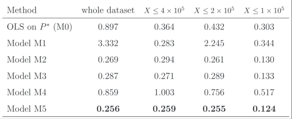
The original data are n = 506 observations on p = 14 variables, medv median value, being the target variable. crim per capita crime rate

• Etape k , on ajoute au Mod`ele M k le r´egresseur qui augmente le plus le R 2 global parmi les r´egresseurs significatifs.. • On it`ere jusqu’`a ce qu’aucun r´egresseur

For regression models with random design, a procedure achieving the bound (1.2) with optimal rate ψ n,M of (L) aggregation can be found in Tsybakov (2003).. For Gaussian white

Alternatively, Alaoui and Mahoney [1] showed that sampling columns according to their ridge leverage scores (RLS) (i.e., a measure of the influence of a point on the

The problem of handling missing data in generalized linear mixed models with correlated covariates is considered when the missing mechanism con- cerns both the response variable and

By construction, the method MI-PLS proposed by Bastien (2008) will not take into account the random effect and then for assessing the contribution of our method we have

Our constructed estimate of r is shown to adapt to the unknown value d of the reduced dimension in the minimax sense and achieves fast rates when d << p, thus reaching the goal