Publisher’s version / Version de l'éditeur: Energy Policy, 59, pp. 133-142, 2013-04-10
READ THESE TERMS AND CONDITIONS CAREFULLY BEFORE USING THIS WEBSITE.
https://nrc-publications.canada.ca/eng/copyright
Vous avez des questions? Nous pouvons vous aider. Pour communiquer directement avec un auteur, consultez la première page de la revue dans laquelle son article a été publié afin de trouver ses coordonnées. Si vous n’arrivez pas à les repérer, communiquez avec nous à PublicationsArchive-ArchivesPublications@nrc-cnrc.gc.ca.
Questions? Contact the NRC Publications Archive team at
PublicationsArchive-ArchivesPublications@nrc-cnrc.gc.ca. If you wish to email the authors directly, please see the first page of the publication for their contact information.
NRC Publications Archive
Archives des publications du CNRC
This publication could be one of several versions: author’s original, accepted manuscript or the publisher’s version. / La version de cette publication peut être l’une des suivantes : la version prépublication de l’auteur, la version acceptée du manuscrit ou la version de l’éditeur.
For the publisher’s version, please access the DOI link below./ Pour consulter la version de l’éditeur, utilisez le lien DOI ci-dessous.
https://doi.org/10.1016/j.enpol.2013.02.030
Access and use of this website and the material on it are subject to the Terms and Conditions set forth at
A model of residential energy end-use in Canada: using conditional
demand analysis to suggest policy options for community energy
planners
Newsham, Guy R.; Donnelly, Cara L.
https://publications-cnrc.canada.ca/fra/droits
L’accès à ce site Web et l’utilisation de son contenu sont assujettis aux conditions présentées dans le site
LISEZ CES CONDITIONS ATTENTIVEMENT AVANT D’UTILISER CE SITE WEB.
NRC Publications Record / Notice d'Archives des publications de CNRC: https://nrc-publications.canada.ca/eng/view/object/?id=20450f55-93e4-4f30-a675-ec0bfa25d45d https://publications-cnrc.canada.ca/fra/voir/objet/?id=20450f55-93e4-4f30-a675-ec0bfa25d45d
A Model of Residential Energy End-Use in Canada:
Using Conditional Demand Analysis to Suggest Policy Options for Community Energy Planners
Guy R. Newshama, PhD and Cara L. Donnelly, PhD
National Research Council Canada, 1200 Montreal Road (M24), Ottawa, Ontario, K1A 0R6, Canada
aCorresponding Author; t: (613) 993-9607; f: (613) 954-3733; e: guy.newsham@nrc-cnrc.gc.ca
Abstract
We applied Conditional Demand Analysis (CDA) to estimate the average annual energy use of various electrical and natural gas appliances, and derived energy reductions associated with certain appliance upgrades and behaviours. The raw data came from 9773 Canadian households, and comprised annual electricity and natural gas use, and responses to >600 questions on dwelling and occupant characteristics, appliances, heating and cooling equipment, and associated behaviours. Replacing an old (>10 years) refrigerator with a new one was estimated to save 100 kWh/yr; replacing an incandescent lamp with a CFL/LED lamp was estimated to save 20 kWh/yr; and upgrading an old central heating system with a new one was estimated to save 2000 kWh/yr. This latter effect was similar to that of reducing the number of walls exposed to the outside. Reducing the winter thermostat setpoint during occupied, waking hours was estimated to lower annual energy use by 200 kWh/oC-reduction, and
lowering the thermostat setting overnight in winter relative to the setting during waking hours (night-time setback) was estimated to have a similar effect. This information may be used by policy-makers to optimize incentive programs, information campaigns, or other energy use change instruments.
Keywords
Residential, appliances, Canada
Research Highlights
Conditional Demand Analysis (CDA) applied to data from 9773 Canadian households Energy savings associated with certain appliance upgrades estimated
Energy savings associated with thermostat behaviours estimated
1. Introduction
1.1 Estimating Appliance Energy Use
As part of a larger project on community energy strategies, we desired to estimate the typical annual energy use of various electrical and natural gas appliances, with the particular goal of deriving the energy reductions associated with appliance upgrades and behaviours.
There are three methods typically used to estimate the energy use of individual appliances. The first is direct sub-metering, in which an energy meter is installed on every (major) appliance in a household. The meters should be left in place to record energy use for a representative period. This process should be repeated in multiple houses, with a sample size representative of the larger population, typically several hundred, and will then yield very high quality data and energy use estimates. However, this method is also very expensive and invasive, and thus its applications have been limited [e.g. Isaacs et al., 2010; de Almeida, 2011; Parker, 2002].
A second approach is engineering estimates. In this case, the basic power draw of an appliance at the important points in its operational cycle are measured (or estimated), and this is conflated with an assumed usage pattern. The usage pattern may come from a defined standard household definition, or may be estimated by other means [NRCan, 2009]. This method has relatively low data requirements, but whereas the power measurements may be made unambiguously, the usage estimates may not accurately describe the range of possible patterns within and between real households.
The third method, and the one used in this paper, is called Conditional Demand Analysis (CDA). This is a purely statistical technique, and relies, in its simplest form, on survey data on total household energy use and appliance ownership. More sophisticated models may be derived with additional survey data on household characteristics, and householder socio-economic variables and behaviours. It is relatively inexpensive and non-invasive for householders, and was particularly attractive to us in this research because the necessary data already existed, having been collected for a different purpose. However, it also has limitations. In the following section we describe the CDA method in more detail.
1.2 Conditional Demand Analysis (CDA)
[1] where,
yi = annual energy use of household i(kWh)
UECij = annual energy use (unit energy consumption) of appliance jin household i(kWh)
Nij = number of appliance jpresent in household i
εi = error term (kWh)
Depending on the appliance under consideration, and the survey data available, this equation may be made more sophisticated by casting UECij as a function of climate, household characteristics, and
householder socio-economic variables and behaviours. With data on a large sample of houses, this equation can then be solved using well-established regression techniques, and most prior applications have used ordinary least squares (OLS). Given that yi and Nijare known from survey data, when the
regression equation is solved the unknown variables UECijare the regression coefficients.
Of course, the estimates are dependent on the quality of the raw data, and householders might not be absolutely accurate in their responses to the survey questions, or might not interpret the questions in a universal manner. This introduces noise into the data and increases error in the estimates.
Further, regression relies on variability in the inputs. For example, if we only have data on whether a household has a refrigerator or not, since almost every modern household has a refrigerator of some kind then there is almost no variability in this input. The consequence is that it will be mathematically impossible to separate out refrigerator energy use from other end uses. The only way around this is to have additional data, such as total number of refrigerators, or refrigerator age, which introduces variability.
A third issue is intercorrelation, particularly with respect to unknown variables. For example, we might know about ownership of dishwashers, but not have data on swimming pool ownership. We can expect a positive relationship between ownership of these: higher income households will tend to have more of both. Thus the CDA estimate of dishwasher energy use may include a portion of the energy used by pools, for which we have no explicit input variable, leading to an overestimate of dishwasher energy use. The same problem can occur between known variables, if they are highly intercorrelated the mathematics of regression may not allocate energy use between them appropriately.
Despite these drawbacks, CDA is widely accepted if applied and interpreted appropriately, and end-use estimates have been shown generally to lie within the range of engineering estimates. CDA is widely used by utilities to forecast loads, and by researchers to explore energy end-use issues.
1.3 Prior CDA Studies
In this section we provide brief descriptions of other applications of CDA in similar circumstances. It would be impractical to list all of the individual variables, interactions, and UECs for each of the studies, nevertheless, these were considered in constructing our models. Aydinalp-Koksal & Ugursal [2008] applied CDA to an earlier vintage of the national Canadian dataset that we used in our analysis, although electricity and natural gas energy use data was available for only 2050 and 1012 households, respectively. Tiedemann [2007] used CDA on data from 791 households in British Columbia to develop a model of electricity use. Lafrance & Perron [1994] used CDA to study the change in major energy end-uses in Quebec using three large samples of households (42000, 24000, and 46000) five years apart. Larsen & Nesbakken [2004] developed a model for electricity use in Norway using data from 1453 households. Berg & McGrath [1988] reviewed several older studies of electricity use in US locations, and in particular a study from Florida with data from 7059 households. Similarly, Sebold & Parris [1989] reviewed 30 separate US CDA studies conducted in the 1980s, and Lawrence & Parti [1984] reviewed 15 separate US CDA studies conducted prior to these, with sample sizes typically of several thousand households. Aigner at al. [1984] used 15-minute whole-house electricity data from 80-132 households for the month of August for three consecutive years, combined with survey data, to estimate daily load profiles for individual appliances. It is also noteworthy that the well-established US RECS (Residential Energy Consumption Survey) uses CDA to generate individual end-use estimates [Battles, 1994]. The results of these studies are summarized in the Discussion section for comparison to our own results. A review of these sources quickly reveals that there is no standard set of variables used as predictors in the regression equation. In each study the surveys were very or subtly different. The list of appliances that respondents were asked to report on varied, as did the properties of these appliances, and the behaviours that householders employed. Nevertheless, there were some common themes in the studies, and we used these to inform our choice of model variables, along with knowledge of engineering principles. Still, the final choice of variables involves some exploratory work including/excluding variables and interpreting the result. Our choices were limited by the content of the survey that provided our data, a survey that we did not play a role in designing.
2. Methods & Procedures 2.1 Survey Data
Our raw data came from the 2007 administration of the Households and the Environment Survey (HES) [StatCan, 2009]. The target group was a geographically representative sample from across Canada (excluding northern territories, Indian reserves, and households of armed forces personnel). Respondents from 21690 households completed the survey via telephone interview. The survey consisted of more than 300 questions on dwelling and occupant characteristics, energy use, water, fertilizers and pesticides, recycling and composting, indoor environment and air quality, and transportation and gasoline use. In addition, in 2007, NRCan partnered with StatCan to administer a supplementary questionnaire on Energy Use (EUS) [StatCan, 2010]. This survey was administered in paper form to all HES households; complete data were obtained from 9773 households. The EUS consisted of more than 300 questions on dwelling and occupant characteristics, household appliances, and HVAC equipment. The EUS also obtained energy use data; data for electricity and gas were monthly and were obtained, in most cases, directly from the utility (with the householder’s permission).
2.2 Climate Data
For household energy use related to space heating and cooling, we introduced a dependency on local climate data. The standard indices used in CDA, and in building energy studies more generally [ASHRAE, 2009, Ch. 14], are heating-degree-days (HDD) and cooling-degree days (CDD), typically to a base temperature of 18 oC (considered the typical outdoor temperature at which there is a transition from
space heating to space cooling)1. Equations are shown below:
[2]
[3] where,
1Prior studies have used various base temperatures, including 18 oC, and there is recognition that there is a wide
range of appropriate base temperatures between buildings, depending on their specific construction and operational characteristics. Nevertheless, for large building populations where specific characteristics are not known, 18oC persists in being the most common choice for base temperature, and HDD and CDD to this base are
HDD18k = heating degree days, base 18 oC in location k
CDD18k = cooling degree days, base 18 oC in location k
= average outdoor temperature in location k on day d (oC)
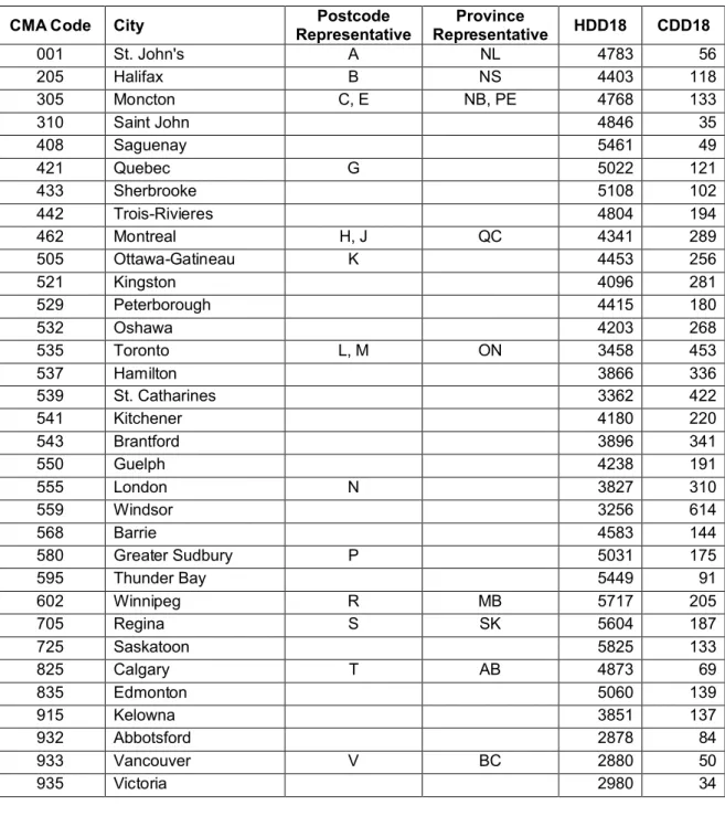
In our dataset, the geographical information for each household was limited to census metropolitan area (CMA, an urban area with a population of 100,000 or more), province, and the first three letters of the postcode. We used data from Environment Canada from 2007 to calculate HDD18 and CDD18 for each CMA. Households with a valid CMA code (N=4663) were assigned the climate data for that CMA. For the remainder we looked next at the postcode, and assigned the climate data for a representative CMA with the same postcode first character. For households that did not provide postcode data (N=820) we assigned the climate data for a representative CMA in the same province. Climate data and geographical assignments are shown in Appendix A.
2.3 Data Cleaning
Our general approach was to remove, or cap, extreme values for the major variables in the model. In common with prior work in this area, we considered univariate outliers only. For electrical energy use, we dropped cases where reported household energy use was more than 4 s.d. from the mean; we also decided that households with energy use of <1000 kWh/yr represented low outliers. We also dropped cases where reported dwelling age, total household income, number of occupants, and dwelling floor area were each more than 4 s.d. from the mean; we also determined that dwellings with a floor area of <400 ft2 represented low outliers. Finally, we dropped cases where reported weeks in the year the
dwelling was occupied was more than 3 s.d. from the mean2. Table 1 summarizes descriptive statistics
for the variables described above in the raw data; mean values following the collective removal of these outliers, and listwise removal of missing values, are shown alongside model results below. Data from the national census indicated national median/mean household income before tax was $53,634/$69,548, and the mean number of occupants per private dwelling was 2.5 [StatCan, 2006]. Based on these metrics our starting sample appears representative of Canadian households generally. However, the results tables indicate that the final model samples were weighted towards households with higher incomes. We also note that the proportion of single-family detached dwellings in our
2We have typically used 3 s.d. as an outlier criterion in other kinds of work [e.g. Veitch et al., 2007]. In this case
we were concerned that excluding outliers on multiple variables with this criterion would erode the sample size too much, so we chose a more liberal criterion for most variables. We retained the 3 s.d. criterion for the absence variable because a more liberal criterion created a minimum value for absence that we judged to be too low.
sample was higher than for Canadian households generally. These biases were likely due to self-selection in the voluntary EUS process.
Table 1. Descriptive statistics for entire sample. Refer to glossary for variable descriptions.
ELECTRICITY
(kWh) NGAS (kWh) HAGE (yrs)
INCOME (x1000 $) NOCC FLOOR_AREA (x 1000 ft2)a N 9773 9773 9303 8946 9553 9773 Mean 12312 12291 36.6 67.6 2.40 2.11 Std. Deviation 8412 15145 25.7 61.8 1.23 1.02 Median 9897 0 32 52.0 2 2.02 Minimum 14 0 0 0 1 0.17 Maximum 61434 102251 207 3000.0 14 8.20
aCanada is officially metric, but Canadian house sizes are almost universally quoted in ft2, and it therefore made
sense in our context to conduct analysis and reporting in these terms; 1000 ft2= 92.9 m2, and our sample mean of
2110 ft2= 196m2.
2.4 Model Development
We followed the process outlined in Aydinalp-Koksal & Ugursal [2008] by first considering logical approaches to modelling individual appliance categories from engineering principles and the data available. Then we combined these categories together into final models, by delivered energy (fuel) type, and tested variations and options on these. For brevity, we do not describe the development and variations of all model options, but will describe the terms in the final models when discussing the results. In general, space heating/cooling appliances were interacted with climate and house size data, and some other appliances were interacted with data on number of occupants, or usage. We included separate terms for both old (>10 years) and new versions of the same appliance (where data permitted)3, as well as additional estimates for the heat loss associated with having all (four) walls
exposed to the outside, and for various thermostat behaviours applied to central heating systems.
After finalizing the electricity model we developed a natural gas model that followed the same form. This aided in comparing the models and interpreting the policy guidance derived from the model outputs, and we reasoned that energy use models should be robust in form where the end uses are identical. There are far fewer appliances that use natural gas, but some, particularly those for space and
3For some appliances, respondents were asked to indicate whether it was Energy Star rated. After exploration, we
chose not to further divide new appliances into Energy Star and non-Energy Star types. The sample sizes in some of these categories were very low, and we were concerned about the accuracy of Energy Star recognition and reporting by the respondents.
water heating, are large users. Outliers were determined in an identical way as for the electricity models, except that we did not exclude very low values of natural gas use: very low use of natural gas is legitimate as many households have few gas appliances.
The dataset did contain information on the use of other fuels, including oil, propane, and wood. These fuels collectively represent only a minor part of total residential energy use nationally (although they are important in some provinces). In principal, similar models could have been developed for these fuels, however, project scope did not allow us to pursue this.
3. Results
3.1 Electricity Model
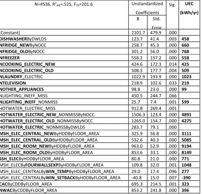
Table 2 shows the output table for the final model (we used SPSS v. 19). The complex model was statistically significant and explains 53 % of the variance in annual electricity use. All of the terms in the final model are statistically significant contributors to the model (using our usual α=0.05 criterion), with two exceptions, as described below. The values in the column labelled “B” are the coefficient estimates of interest, from which UECs can be derived. An N preceding an independent variable name (see glossary for variable definitions) indicates that it represents the number of such appliances reported for the household, and therefore can have a value greater than 1. Independent variable names not preceded by an N indicate whether at least one appliance was owned, and therefore can have a maximum value of 1; in these cases, ownership of more than one such appliance would be very rare. Table 3 shows mean values for each of the principal variables included in the model, and only for the cases included in the model.
Table 2. Output of regression model for electricity use (complex). The final column shows the resulting UEC estimate for the associated appliance or behaviour shown in bold type.
N=4536, R2 adj=.525, F25=201.6 Unstandardized Coefficients Sig. UEC (kWh/yr) B Std. Error (Constant) 2101.7 479.9 .000 DISHWASHERByDWLDS 123.7 41.4 .003 458 NFRIDGE_NEWByNOCC 258.7 45.3 .000 660 NFRIDGE_OLDByNOCC 301.2 56.0 .000 768 NFREEZER 558.2 157.2 .000 558 NCOOKING_ELECTRIC_NEW 424.6 172.3 .014 425 NCOOKING_ELECTRIC_OLD 508.5 177.7 .004 509 NLAUNDRY_ELECTRIC 1022.9 193.9 .000 1023 NTELEVISION 218.9 102.6 .033 219 NOTHER_APPLIANCES 98.8 23.0 .000 99 NLIGHTING_INEFF_MISS 450.5 244.7 .066 NLIGHTING_INEFF_NONMISS 25.7 7.4 .001 599 HOTWATER_ELECTRIC_MISS 912.8 269.4 .001 HOTWATER_ELECTRIC_NEW_NONMISSByNOCC 1506.3 123.4 .000 4891 HOTWATER_ELECTRIC_OLD_NONMISSByNOCC 1265.0 154.7 .000 4275 HOTWATER_ELECTRIC_NONMISSByDWLDS 283.7 79.1 .000 MSH_ELEC_CENTRAL_NEWByHDDByFLOOR_AREA 325.9 56.8 .000 3111 MSH_ELEC_CENTRAL_OLDByHDDByFLOOR_AREA 532.6 40.3 .000 5085 MSH_ELEC_ROOM_NEWByHDDByFLOOR_AREA 963.0 52.9 .000 9194 MSH_ELEC_ROOM_OLDByHDDByFLOOR_AREA 853.6 33.1 .000 8149 SSH_ELECByHDDByFLOOR_AREA 80.8 21.0 .000 771 MSH_ELECByFOURWALLSEXPByHDDByFLOOR_AREA 109.8 32.0 .001 1048 MSH_ELEC_CENTRALByWIN_TEMPByHDDByFLOOR_AREA 29.0 17.4 .096 277 MSH_ELEC_CENTRALByWIN_SETBACKByHDDByFLOOR_AREA -40.8 15.0 .007 -390 CACByCDDByFLOOR_AREA 695.3 214.5 .001 323 NWACByCDDByFLOOR_AREA 853.2 241.8 .000 396
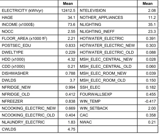
Table 3. Mean values for variables and cases used in regression model for electricity use (complex).
Mean Mean
ELECTRICITY (kWh/yr) 12412.5 NTELEVISION 2.08
HAGE 34.1 NOTHER_APPLIANCES 11.2 INCOME (x1000$) 73.6 NLIGHTING 35.1 NOCC 2.55 NLIGHTING_INEFF 23.3 FLOOR_AREA (x1000 ft2) 2.21 HOTWATER_ELECTRIC 0.391 POSTSEC_EDU 0.833 HOTWATER_ELECTRIC_NEW 0.303 DWELTYPE 0.229 HOTWATER_ELECTRIC_OLD 0.088 HDD (x1000) 4.32 MSH_ELEC_CENTRAL_NEW 0.028 CDD (x1000) 0.21 MSH_ELEC_CENTRAL_OLD 0.060 DISHWASHER 0.788 MSH_ELEC_ROOM_NEW 0.039 DWLDS 3.7 MSH_ELEC_ROOM_OLD 0.150 NFRIDGE_NEW 0.994 SSH_ELEC 0.182 NFRIDGE_OLD 0.412 FOURWALLSEXP 0.455 NFREEZER 0.838 WIN_TEMP -0.417 NCOOKING_ELECTRIC_NEW 0.669 WIN_SETBACK 2.00 NCOOKING_ELECTRIC_OLD 0.404 CAC 0.358 NLAUNDRY_ELECTRIC 1.83 NWAC 0.21 CWLDS 4.75
In cases where an appliance variable is interacted with another variable, one obtains the UEC estimate for the appliance by multiplying the value in the “B” column by the mean value of the interaction variable(s). For example, dishwasher ownership is interacted with number of dishwasher loads per week, so UEC estimate for mean dishwasher energy use is 123.7 x 3.7 = 458 kWh/yr. Similarly, number of refrigerators was interacted with number of household occupants. The number of occupants is a common interaction variable in prior cited studies. Some authors have found that non-linear expressions for number of occupants worked better, with the increase in energy use per additional occupant declining as the number of occupants increases (e.g. square-root or logarithmic variants [e.g. Manitoba Hydro, 2011; Tiedemann, 2007]). We tried these, but saw little benefit. For lighting, the UEC is the estimated energy use per lamp, multiplied by the average number of lamps per house.
The three electric cooking appliances (stove, cooktop, and oven) were combined into a single electric cooking variable, as cooktop and oven ownership was extremely small. Stove ownership was very high, but the combined variable, which had a maximum value of 3, introduced enough variability into the cooking-related appliance variable. Similarly we combined clothes washers and dryers into a single variable. Ownership of washers and dryers was very high, and adding them to the model as separate variables introduced destabilizing effects, as might be expected; Tiedemann [2007] had a combined laundry appliance variable for a CDA model for BC, Canada, presumably for similar reasons. We also combined ownership of a variety of smaller appliances into a single “other” variable. This included microwaves, computers, monitors, TV entertainment devices, audio equipment, phones, and watercoolers. In this case, the value in the “B” column represents the mean use of any one of these appliances, we cannot distinguish among them with this model.
For water heating, we included variables to separately account for the usage by the dishwasher, dependent on dishwasher loads, and usage for other purposes (e.g. hygiene), dependent on number of occupants. The total energy use estimate for water heaters is the sum of these components.
Main space heating was interacted with both heating-degree-days and household floor area (as a correlate for wall area), as suggested by heat loss theory. We used separate variables for households with central space heat and room-level space heat, to parallel the obvious similar separation for air conditioning. Central space heating included hot air, hot water boiler, and heat pump systems; room-level space heat included baseboards and radiant heat systems. Supplemental electric space included use of any of supplementary electric baseboards, portable heaters, electric fireplace, supplementary radiant floor heating, or supplementary electric furnace was indicated.
For main space heating, we included an additional variable with an interaction that coded for a household with all (four) walls exposed to the outside; this included mobile homes, and single detached houses without an attached garage. For central main space heating systems we included additional variables with interactions related to thermostat behaviour. The first related to reported thermostat setting (in Celsius) in the winter when someone was at home and awake. We took the reported value and subtracted 21 (the median value) to represent a deviation from median behaviour. The second related to reported thermostat night-time setback behaviour, which was the reported thermostat setting in the winter when someone was at home and awake minus the thermostat setting in the winter during the night. Note that although the interaction related to thermostat setting was not statistically significant it was retained because: it was a useful counterpoint to the setback interaction variable; its
inclusion improved the rest of the model; its coefficient is reasonable; although our practice is to use α=0.05, authors of some prior CDA studies have accepted variables with values of p<0.1 [e.g. Aydinalp-Koksal & Ugursal, 2008; Lafrance & Perron, 1994]; and, the equivalent term was significant in the gas model.
Freezers and laundry appliances were not divided into new and old categories as this did not help with model stability, and because manufacturers’ data suggested [NRCan, 2011a] little change in energy use per new freezer over the past 20 years. Air-conditioning appliances were not divided into new and old for reasons related to model stability.
Note that we included two specific variables that coded for missing data. For most variables, we took a conservative approach and excluded cases with a missing value on any of the input variables from the analyses. However, for two variables (certain lighting types, and water heater fuel type) the number of missing values was quite large and, in combination with the removal of outliers, reduced the sample size by up to two-thirds. For these we employed the missing indicator method. For example, if there are missing data for a variable X, one creates a new dummy variable X_MISS. If a household had missing data for variable X then X is recoded to 0, and X_MISS is coded as 1; if a household had non-missing data for X then X is unchanged, and X_MISS is coded as 0. X_MISS is then included as a predictor in the regression equation. This approach preserves cases, but it is conceptually unappealing in that the dummy variable has no real-world meaning, although one would hope that its coefficient estimate approximates the average energy use for households with non-missing data. This method might not be attractive in all applications [van der Heijden et al., 2006], but it has been used to advantage in prior CDA analyses [Bartels & Fiebig, 2000; Manitoba Hydro, 2011].
For lighting, the variables related to efficient lighting (fluorescent) were not statistically significant and were thus dropped from the model, whereas the inefficient lighting variable (incandescent) was retained. Fluorescent technologies are typically four to five times more efficient than incandescent technologies, and thus the mean energy use of a single fluorescent lamp would be too small to be resolved by the model. The missing dummy code variable for inefficient lighting was retained, despite having a p>0.05, because dropping it would mean cutting the overall sample size substantially and thus compromising other end-use estimates.
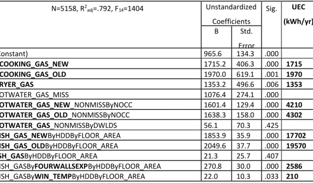
The gas model had the same form as the electricity model, with some small deviations. We included an additional missing data dummy code, because there were households that had a relatively high gas use (our criterion was 10000 kWh/yr) but reported not using natural gas as their main space heating fuel. We reasoned that such high gas use would be very difficult to achieve without using gas for space heat. We did not have other data that would allow us to confidently recode the main space heating fuel as gas, so we chose to recode the data with a missing dummy code instead. This substantially increased the variability explained by the model. We included a separate variable for clothes dryer; gas washers do not exist, and gas dryers are rare, and thus the universal ownership problem with electric laundry appliances did not apply here. Dryers were not divided into new and old categories to parallel the decision made in the electricity model with regard to laundry appliances.
Table 4 shows the output table for the final model. This model is statistically significant and explains 79 % of the variance in annual gas use. All of the terms in the final model are statistically-significant contributors to the model, with two exceptions: the term for interaction of water heating and dishwasher loads, and the term for supplemental space heat. We left these in to maintain parallelism with the electricity model. Table 5 shows descriptive statistics for each of the variables included in the model, and only for the cases included in the model.
Table 4. Output of regression model for gas use (complex). The final column shows the resulting UEC estimate for the associated appliance or behaviour shown in bold type.
N=5158, R2 adj=.792, F14=1404 Unstandardized Coefficients Sig. UEC (kWh/yr) B Std. Error (Constant) 965.6 134.3 .000 NCOOKING_GAS_NEW 1715.2 406.3 .000 1715 NCOOKING_GAS_OLD 1970.0 619.1 .001 1970 DRYER_GAS 1353.2 496.6 .006 1353 HOTWATER_GAS_MISS 1076.4 274.1 .000 HOTWATER_GAS_NEW_NONMISSByNOCC 1601.4 129.4 .000 4210 HOTWATER_GAS_OLD_NONMISSByNOCC 1638.3 158.0 .000 4302 HOTWATER_GAS_NONMISSByDWLDS 56.1 70.3 .425 MSH_GAS_NEWByHDDByFLOOR_AREA 1853.9 35.9 .000 17702 MSH_GAS_OLDByHDDByFLOOR_AREA 2049.6 37.7 .000 19570 SSH_GASByHDDByFLOOR_AREA 21.3 25.7 .407 MSH_GASByFOURWALLSEXPByHDDByFLOOR_AREA 270.8 30.0 .000 2586 MSH_GASByWIN_TEMPByHDDByFLOOR_AREA 22.0 10.3 .033 210
MSH_GASByWIN_SETBACKByHDDByFLOOR_AREA -22.8 8.8 .009 -218
NGAS_HEAT_MISS 21202.5 412.9 .000
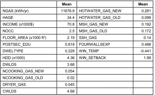
Table 5. Mean values for variables and cases used in regression model for gas use (complex).
Mean Mean
NGAS (kWh/yr) 11676.9 HOTWATER_GAS_NEW 0.281
HAGE 34.4 HOTWATER_GAS_OLD 0.099 INCOME (x1000$) 70.8 MSH_GAS_NEW 0.192 NOCC 2.5 MSH_GAS_OLD 0.172 FLOOR_AREA (x1000 ft2) 2.19 SSH_GAS 0.14 POSTSEC_EDU 0.819 FOURWALLSEXP 0.488 DWELTYPE 0.229 WIN_TEMP -0.441 HDD (x1000) 4.36 WIN_SETBACK 1.99 DWLDS 3.68 NCOOKING_GAS_NEW 0.054 NCOOKING_GAS_OLD 0.02 DRYER_GAS 0.045 CWLDS 4.68 4. Discussion
4.1 Comparison of UECs to Other Sources
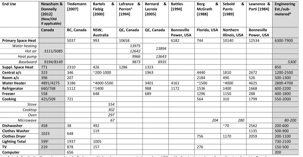
For electric appliances, there are several studies to which we can compare our results. Table 6 summarizes the UECs for each appliance type from prior CDA studies, sub-metering, and engineering estimates, and compares them to values derived from our analysis. Note that previous work did not consider the age effects or behaviours that we addressed in our more complex model.
In addition to the values in Table 6, we can generate additional, simplified estimates for comparison. For example a 120 W TV [CNET, 2010] on for 4 hrs/day uses 175 kWh/yr. For lighting, the most common single lamp type in residences is probably the 60W incandescent [Navigant, 2002, Appendix D]. Single fluorescent lamps are usually <30W, but single halogen lamps may be 25W or 50W, and can be as high as 150W. The most commonly used lamps are on ~3 hrs/day, but a reasonable average might be 1 hr/day [Gaffney et al., 2010; Navigant, 2002 Appendix D]. These assumptions yield an average use per lamp of 18.3 kWh/yr. Sub-metering of 12 residential a/c units in southern Ontario, representing a CDD
above the average for our sample, showed an average energy use for cooling of 520 kWh/yr [Saldanha & Beausoleil-Morrison, 2012].
For gas appliances, we were not able to find citable studies to which we can compare our results. However, we were given the results of a CDA gas analysis from a large Canadian utility [Manitoba Hydro, 2011]. For gas cooking, our estimate is substantially higher than that for electric cooking, but is
substantially lower than the value provided by Manitoba Hydro (2752 kWh/yr). For gas dryers, our estimate is substantially higher than that for a single electric laundry appliance, but this may be partially explained by the lower efficiency of delivered energy from gas compared to electric. Our estimate is in good agreement with the value provided by Manitoba Hydro (1799 kWh/yr). For gas water heating, our estimate is similar to our estimate for electric water heating, and is a somewhat lower than the value provided by Manitoba Hydro (5335 kWh/yr). For main space heating, an estimate derived from the value provided by Manitoba Hydro (inputting the same average house size as in our sample, and assuming a mid-efficiency furnace) was 26900 kWh/yr. Substituting the HDD18 value for Winnipeg into our estimate yielded a value of ~25000 kWh/yr.
Overall, our UEC estimates are in good agreement with the range of values from prior studies, and form a better complete set than any single prior study. The only major exception was for central electric heating. But note that for Canada as a whole this type of main space heating is rare, and the single most common main space heating type in Canada is natural gas.
Table 6. Comparison of our UEC estimates for electric appliances to those from prior CDA studies.
End Use Newsham &
Donnelly [2012]
(New/Old if applicable)
Tiedemann
[2007] Bartels Fiebig &
[2000] Lafrance & Perrona [1994] Bernard & Lacroix [2005] Battles
[1994] Berg McGrath &
[1988]
Sebold &
Parris [1989]
Lawrence &
Parti [1984] Engineering
Est./sub-meteredb
Canada BC, Canada NSW,
Australia QC, Canada QC, Canada Bonneville Power, USA Florida, USA Northern Illinois, USA Bonneville Power, USA
Primary Space Heat 5037 993 10658 6182 744 10140 12534 6300-7900
Water heating
3111/5085 13975 13894
Hot air 12642
Heat pump 9966 13643
Baseboard 9194/8149 9873 8935 5300
Suppl. Space Heat 771 2310 426 1286 1323 850
Central a/c 323 346 ~200-1000 1963 4440 1810 2672 1200-2500 Room a/c 396 207 2184 490 526 500-1300 Water Heater 4891/4275 3186 ~4000-5500 3401 4161 ~1500 ~4000 4625 2800-4700 Refrigerator 660/768 1112 ~1400 988 1172 1536 1400 1668 600-2200 Freezer 558 648 689 1296 1150 288 400-1800 Cooking 425/509 721 564 310 1799 550-2000 Stove 554 Cooktop 302 Oven 297 Microwave 67 204 280 80-200 Dishwasher 458 38 492 ~70 2562 200-600 Clothes Washer 1023 648 119 1135 500-900 Clothes Dryer 756 1170 2059 200-1100 Lighting Total 599c 1937 1005 730-2100 TV 219 878 157 276 150-500 Computer 656 200
asingle family dwelling sub-sample only; bwhere multiple values were reported, we chose UECs with climate dependence from climates closest to Canada; cfor incandescent and halogen only
4.2 Informing Potential Policy Actions
Our results provide estimates for the policy-maker on the potential energy savings associated with various actions, information which may then be used to optimize incentive programs or other
instruments. Table 7 summarizes the appliance substitutions, behaviours and other choices with their energy effects as estimated in our models and rounded for ease of interpretation. In this table we highlight only those effects that appear to be reliable4.
Table 7. Summary of potential energy saving actions and behaviours, for policy consideration.
Appliance / End use Action Energy saving
(kWh/yr) Common Policy Option
Refrigerator Replace Old with New 100 Incentive and free disposal [e.g. Hydro Ottawa, 2012a]
Electric Cooking Equipment Replace Old with New 100 Incentive and free disposala
Lighting Replace incandescent
with CFL (or LED) 20/lamp Incentive [e.g. Hydro Ottawa, 2012b]
b
Electric Main Space
Heating Replace Old Central system with New 2000 Incentive and free disposal
c
Gas Main Space Heating Replace Old system
with New 2000 Incentive and free disposal
Electric Main Space
Heating Reduce number of walls exposed to exterior 1000 Zoning Gas Main Space Heating Reduce number of walls
exposed to exterior 2500 Zoning Gas Main Space Heating Lower thermostat
during waking period 200 /
oC
reduction Information campaign
d
Electric Main Space
Heating Night-time thermostat setback in winter 400/
oC
setback Incentive for programmable thermostat, and information campaign Gas Main Space Heating Night-time thermostat
setback in winter 200/
oC
setback Incentive for programmable thermostat, and information campaign aThe model also suggests savings by replacing old gas cooking appliances with new appliances, but the standard
error of these estimates was very large
bA reasonable estimate of energy saving associated with replacing an inefficient lamp (incandescent) with an
efficient one (fluorescent, or LED) may be based on the efficacy difference, which is typically 4-5x better for efficient lamps
cThe model also suggests substantial savings from replacing room-level heating with a central system, this is an unlikely option in renovation, but could be a reasonable requirement for new build
dThe model suggested a similar saving for houses with electric main space heating, but the effect was not
statistically-significant at the 0.05 level (p=.096)
4Note that although the new/old estimates by appliance type are statistically significant effects, generally in the
expected direction and have a plausible magnitude, in most cases there is overlap of standard errors. The larger the overlap, the less confidence we can have that the differences are genuine and not just due to chance.
Note that although the UEC estimate for central electric heating was somewhat low, the saving
associated with replacing an old central heating system with a new one was ~2000 kWh/yr whether the fuel type was electricity or natural gas. Note that the reduction in UEC in going from an old to a new gas furnace is similar to the effect that might be expected with improvements in furnace efficiencies from low to mid, or from mid to high [CMHC, 2011]. The effect of having four walls exposed scales
approximately with the UEC for heating by fuel. There is no obvious reason why the effect of setting back the thermostat at night would differ by heating system fuel type. A conservative estimate might be 200/oC for both fuel types, about the same as the effect of increasing thermostat setting during daytime,
occupied hours.
It is interesting to compare the magnitude of energy saving estimates. For example, there has been considerable effort invested in lamp replacement programs, and even looming legislation [NRCan, 2011b]. However, one would have to replace 20 lamps to save the same energy as the mean night-time thermostat setback of 2 oC. If the setback is achieved via the installation of a programmable thermostat
(of course, one can also realise the saving with diligent manual actions), it can then be used for other energy-savings actions, such as automated demand response [Newsham et al., 2011]. On the other hand, replacing five lamps may be far easier than replacing a refrigerator or electric cooking equipment. Nevertheless, there might be other reasons to pursue one action over another, for example, replacing an old refrigerator might prevent CFC leakage.
Our analysis also highlights actions that seem less likely to save energy. For example, our results suggest that new electric water heaters use more energy than older models. This could be due to error in the model, or because water heating correlates with another variable not represented in the model, or because newer water heaters tend to be larger than older ones; we cannot distinguish between these possibilities with the data we have. Also, we see a substantial improvement in energy use for newer central electric heating systems but not for room-based systems. Room-level systems are essentially resistance heaters, and there is little improvement in heating efficiency possible with newer models. Central systems also include fans, pumps, boilers, compressors, etc., which are capable of substantial improvement over time. In fact, the estimate for newer room-based systems is a little higher than for older systems, this may be because newer systems tend to be in newer dwellings, which tend to be bigger and thus have a greater volume to heat.
5. Conclusions
Our results suggest that Conditional Demand Analysis (CDA) is a useful adjunct to sub-metering and engineering calculations for estimating the typical annual energy use of various electrical and gas appliances. Further, estimates of the energy reduction effect of appliance upgrades and some behaviours may be derived. These estimates might help to identify incentives and policies most likely to be cost-effective.
Acknowledgements
This research received financial support from the National Research Council Canada, and Natural Resources Canada Clean Energy Fund (CEF). In addition, we are indebted to the following people for their help with this work: Ken Church, Raymond Boulter, Dennis Jackson, Dominic Demers, Andrew Kormylo, Yantao Liu (all NRCan), and Gordon Dewis (Statistics Canada). We are also grateful to Dr. Jennifer Veitch (NRC) for her advice throughout the project and her thorough review of the final report.
References
ASHRAE. 2009. Handbook Fundamentals. American Society of Heating, Refrigerating and Air-Conditioning Engineers, Atlanta USA.
Aigner, D.J., Sorooshian, C., Kerwin, P. 1984. Conditional demand analysis for estimating residential end-use load profiles. The Energy Journal, 5(3), 81-97.
Aydinalp-Koksal, M., Ugursal, V.I. 2008. Comparison of neural network, conditional demand analysis, and engineering approaches for modeling end-use energy consumption in the residential sector. Applied Energy, 85, 271-296.
Bartels, R., Fiebig, D.G. 2000. Residential end-use electricity demand: results from a designed experiment. The Energy Journal, 21(2), 51-81.
Battles, S.J. 1994. Validation of conditional demand estimates: does it lead to model improvements? Proceedings of the ACEEE Summer Study on Energy Efficiency in Buildings (Pacific Grove, CA, USA), 7.13-7.22.
Berg, S.V., McGrath, M.J. 1988. Survey of household end-use consumption. Public Utility Research Center, Working Paper 88-10.
Bernard, J.-T., Lacroix, G. 2005. Conditional demand analysis: tests for homoscedasticity and uniformity. U. Laval, GREEN paper 2005-4. URL: http://www.green.ecn.ulaval.ca/chaire/2005/2005-4.pdf(last accessed 2012-04-25). CMHC. 2011. Replacing Your Furnace. Canada Mortgage and Housing Corporation, fact sheet. URL:
http://www.cmhc-schl.gc.ca/en/co/renoho/refash/refash_018.cfm(last accessed 2012-04-03).
CNET. 2010. The chart: HDTV power consumption compared. URL: http://reviews.cnet.com/green-tech/tv-consumption-chart/?tag=mncol;txt(last accessed 2012-04-02)
de Almeida, A., Fonseca, P., Schlomann, B., Feilberg, N. 2011. Characterization of the household electricity consumption in the EU, potential energy savings and specific policy recommendations. Energy and Buildings, 43, 1884-1894.
Gaffney, K., Goldberg, M., Tanimoto, P., Johnson, A. 2010. I know what you lit last summer: results from California's residential lighting metering study. Proceedings of ACEEE Summer Study on Energy Efficiency in Buildings (Pacific Grove, CA, USA), 9.80-9.91.
Hydro Ottawa. 2012a. Fridge and Freezer Pickup, saveONenergy programs. URL:
http://www.hydroottawa.com/residential/saveonenergy/programs-and-incentives/fridge-and-freezer/(last accessed 2012-04-03)
Hydro Ottawa. 2012b. Downloadable Coupons, saveONenergy programs. URL:
http://www.hydroottawa.com/residential/saveonenergy/programs-and-incentives/coupons/downloadable-coupons/ (last accessed 2012-04-03)
Isaacs, N.P. (ed.), Camilleri, M., Burrough, L., Pollard A., Saville-Smith, K., Fraser, R., Rossouw, P., Jowett, J. 2010. Energy use in New Zealand Households: Final report on the Household Energy End-use Project (HEEP). BRANZ Study Report 221. URL:
http://www.branz.co.nz/cms_show_download.php?id=a9f5f2812c5d7d3d53fdaba15f2c14d591749353(last accessed 2012-01-18)
Lafrance, G., Perron, D. 1994. Evolution of residential electricity demand by end-use in Quebec 1979-1989: a conditional demand analysis. Energy Studies Review, 6(2), 164-173.
Larsen, B.M., Nesbakken, R. 2004. Household electricity end-use consumption: results from econometric and engineering models. Energy Economics, 26, 179-200.
Lawrence, A.G., Parti, M. 1984. Survey of conditional energy demand models for estimating residential unit energy consumption coefficients. EPRI Report EA-3410. Electric Power Research Institute, Palo Alto, USA.
Manitoba Hydro. 2011. Market Forecast Department, personal communication.
Navigant. 2002. U.S. Lighting Market Characterization, Volume I: National Lighting Inventory and Energy Consumption Estimate. URL: http://apps1.eere.energy.gov/buildings/publications/pdfs/ssl/lmc_vol1_final.pdf
(last access 2012-04-02)
Newsham, G.R., Birt, B., Rowlands, I.H. 2011. A comparison of four methods to evaluate the effect of a utility residential air-conditioner load control program on peak electricity use. Energy Policy, 39 (10), pp. 6376-6389. NRCan. 2009. How the Ratings on the EnerGuide Label Are Established. Natural Resources Canada, Office of Energy Efficiency. URL: http://oee.nrcan.gc.ca/equipment/appliance/15538(last accessed 2012-04-02)
NRCan. 2011a. Energy Consumption of Major Household Appliances Shipped in Canada, Summary Report – Trends for 1990–2009. Natural Resources Canada, Office of Energy Efficiency. URL:
http://oee.nrcan.gc.ca/publications/statistics/cama11/index.cfm(last accessed 2012-04-03)
NRCan. 2011b. Phase-Out of Inefficient Light Bulbs. Natural Resources Canada, Office of Energy Efficiency. URL:
http://oee.nrcan.gc.ca/regulations/17723(last accessed 2012-04-03)
Parker, D.S. 2002. Research highlights from a large scale residential monitoring study in a hot climate. Proceedings of International Symposium on Highly Efficient Use of Energy and Reduction of its Environmental Impact (Osaka, Japan), 108-116.
Saldanha, N., Beausoleil-Morrison, I. 2012. Measured end-use electric load profiles for 12 Canadian houses at high temporal resolution. Energy and Buildings, in press.
Sebold, F.D., Parris, K.M. 1989. Residential end-use energy consumption: a survey of conditional demand estimates. EPRI Report No. CU-6487.
StatCan. 2006. 2006 Census. Statistics Canada. URL: http://www12.statcan.ca/census-recensement/2006/index-eng.cfm(last accessed 2012-04-03)
StatCan. 2009. Households and the Environment Survey, 2007. Statistics Canada. URL:
http://www.statcan.gc.ca/pub/11-526-x/11-526-x2009001-eng.htm
StatCan. 2010. Households and the Environment: Energy Use, 2007. Statistics Canada. URL:
http://www.statcan.gc.ca/pub/11-526-s/11-526-s2010001-eng.htm
Tiedemann, K. 2007. Using conditional demand analysis to estimate residential energy use and energy savings. Proceedings of the ECEEE Summer Study (La Colle sur Loup, France), 1279-1283.
van der Heijden, G.J.M.G., Donders, A.R.T., Stijnen, T., Moons, K.G.M. 2006. Imputation of missing values is superior to complete case analysis and the missing indicator method in multivariable diagnostic research: a clinical example. Journal of Clinical Epidemiology, 59, 1102-1109.
Veitch, J.A., Charles, K.E., Farley, K.M.J., Newsham, G.R. 2007. A Model of satisfaction with open-plan office conditions: COPE field findings. Journal of Environmental Psychology, 27 (3), 177-189.
Glossary
Here we provide definitions of the basic variables used in the overall energy models and ownership models. Interactions of these variables are also used in the energy models.
CAC Dummy code for ownership of central air conditioning
CDD Number of cooling degree days (base 18 oC) (x1000) CWLDS Number of clotheswasher loads per week
DISHWASHER Dummy code for dishwasher ownership (for all ownership dummy
codes 1=ownership; 0=no ownership)
DRYER_GAS Dummy code for ownership of gas clothes dryer DWELTYPE Type of dwelling (0=single-family detached; 1=other) DWLDS Number of dishwasher loads per week
ELECTRICITY Total annual electricity use for dwelling (kWh/yr)
FLOOR_AREA Total dwelling floor area, including finished basement (x 1000 ft2) FOURWALLSEXP
Dummy code indicating if dwelling had all walls exposed to the exterior climate (1=mobile homes and single detached houses without attached garages; 0=all other)
HAGE Age of dwelling (years)
HDD Number of heating degree days (base 18 oC) (x1000) HOTWATER_ELECTRIC_MISS Dummy code for missing data in water heater fuel type HOTWATER_ELECTRIC_NEW_NONMISS Dummy code for an electric water heater ≤ 10 years old
HOTWATER_ELECTRIC_NONMISS Dummy code for ownership of an electric water heater (missing
data coded as 0)
HOTWATER_ELECTRIC_OLD_NONMISS Dummy code for an electric water heater > 10 years old HOTWATER_GAS Dummy code for ownership of a gas water heater HOTWATER_GAS_MISS Dummy code for missing data in water heater fuel type HOTWATER_GAS_NEW_NONMISS Dummy code for a gas water heater ≤ 10 years old
HOTWATER_GAS_NONMISS Dummy code for ownership of a gas water heater (missing data
coded as 0)
HOTWATER_GAS_OLD_NONMISS Dummy code for a gas water heater > 10 years old INCOME Total household income, before tax (x1000 $)
MSH_ELEC Dummy code for ownership of electric main space heating MSH_ELEC_CENTRAL Dummy code for ownership of centralized electric main space
heating (including furnace, boiler, heat pump)
MSH_ELEC_CENTRAL_NEW Dummy code for centralized electric main space heating ≤ 10
years old
MSH_ELEC_CENTRAL_OLD Dummy code for centralized electric main space heating > 10
years old
MSH_ELEC_ROOM Dummy code for ownership of room-level electric main space
heating (including baseboards, radiant)
MSH_ELEC_ROOM_NEW Dummy code for room-level electric main space heating ≤ 10
years old
years old
MSH_GAS Dummy code for ownership of gas main space heating MSH_GAS_NEW Dummy code for gas main space heating ≤ 10 years old MSH_GAS_OLD Dummy code for gas main space heating > 10 years old NCOOKING_ELECTRIC_NEW Number of electric cooking appliances ≤ 10 years old NCOOKING_ELECTRIC_OLD Number of electric cooking appliances > 10 years old NCOOKING_GAS_NEW Number of gas cooking appliances ≤ 10 years old NCOOKING_GAS_OLD Number of gas cooking appliances > 10 years old NFREEZER Number of stand-alone freezers in dwelling
NFRIDGE_NEW Number of refrigerators in dwelling that were ≤ 10 years old NFRIDGE_OLD Number of refrigerators in dwelling that were > 10 years old NGAS Total annual natural gas use for dwelling (kWh/yr)
NGAS_HEAT_MISS Dummy code for dwellings with >10000 kWh/yr of natural gas
use, but no reported gas main space heating
NLAUNDRY_ELECTRIC Total number of electric laundry appliances (including clothes
washers and dryers) in dwelling
NLIGHTING Total number of lamps (including incandescent, halogen, regular
fluorescent, and compact fluorescent) in dwelling
NLIGHTING_INEFF Total number of inefficient lamps (including incandescent,
halogen) in dwelling
NLIGHTING_INEFF_MISS Dummy code for missing data in inefficient lamp types
(1=missing; 0=non missing)
NLIGHTING_INEFF_NONMISS
Total number of inefficient lamps (including incandescent, halogen) in dwelling (where 0 indicates a dwelling with missing data)
NOCC Number of household occupants
NOTHER_APPLIANCES
Total number of small appliances (including computers,
microwaves, home theatres, DVD players, VCRs, stereos, portable stereos, water coolers, computer monitors, printers, TV set-top boxes, game consoles, and phones) in dwelling
NTELEVISION Total number of televisions in dwelling
NWAC Total number of portable (window) air conditioners in dwelling POSTSEC_EDU Dummy code for at least some post-secondary education (1) vs.
high-school diploma or less (0)
SSH_ELEC Dummy code for supplementary electric space heating SSH_GAS Dummy code for supplementary gas space heating
WIN_SETBACK Thermostat setting in winter when the occupants are present and
awake minus setting at night during sleep (oC)
WIN_TEMP Thermostat setting in winter when the occupants are present and
Appendix A
Table A1. Canadian cities classified as a census metropolitan area (CMA), along with 2007 climate metrics. Cities whose climate data was used to represent a given postcode or province are also shown.
CMA Code City RepresentativePostcode RepresentativeProvince HDD18 CDD18
001 St. John's A NL 4783 56 205 Halifax B NS 4403 118 305 Moncton C, E NB, PE 4768 133 310 Saint John 4846 35 408 Saguenay 5461 49 421 Quebec G 5022 121 433 Sherbrooke 5108 102 442 Trois-Rivieres 4804 194 462 Montreal H, J QC 4341 289 505 Ottawa-Gatineau K 4453 256 521 Kingston 4096 281 529 Peterborough 4415 180 532 Oshawa 4203 268 535 Toronto L, M ON 3458 453 537 Hamilton 3866 336 539 St. Catharines 3362 422 541 Kitchener 4180 220 543 Brantford 3896 341 550 Guelph 4238 191 555 London N 3827 310 559 Windsor 3256 614 568 Barrie 4583 144 580 Greater Sudbury P 5031 175 595 Thunder Bay 5449 91 602 Winnipeg R MB 5717 205 705 Regina S SK 5604 187 725 Saskatoon 5825 133 825 Calgary T AB 4873 69 835 Edmonton 5060 139 915 Kelowna 3851 137 932 Abbotsford 2878 84 933 Vancouver V BC 2880 50 935 Victoria 2980 34