Towards an Intelligent Predictive Model for Analyzing Spatio-Temporal Satellite Image Based on Hidden Markov Chain

(1)

Towards an Intelligent Predictive Model for Analyzing

Spatio-Temporal Satellite Image Based

on Hidden Markov Chain

Houcine Essid1,2, Imed Riadh Farah1,3, Vincent Barra2

1_{Research Laboratory in Computer Integrated Documentation and Arabized-Documentiel Geniuses and Software, National} School of Computer Science Campus, Universitaire de Manouba, Tunis, Tunisie

2_{Limos, Laboratory of Computer Modeling and System Optimization UMR CNRS 6158-Campus Scientifique des} Cézeaux-Office, Aubiere, France

3_{TELECOM-Bretagne, Département ITI Technopôle Brest Iroise, Brest, France} Email: Houcine.essid@isima.fr, riadh.farah@ensi.rnu.tn, vincent.barra@isima.fr

Received May 5, 2013; revised June 5, 2013; accepted July 8, 2013

Copyright © 2013 Houcine Essid et al. This is an open access article distributed under the Creative Commons Attribution License, which permits unrestricted use, distribution, and reproduction in any medium, provided the original work is properly cited.

ABSTRACT

Nowadays remote sensing is an important technique for observing Earth surface applied to different areas such as, land use, urban planning, remote monitoring, real time deformation of the soil that can be associated with earthquakes or landslides, the variations in thickness of the glaciers, the measurement of volume changes in the case of volcanic erup- tions, deforestation, etc. To follow the evolution of these phenomena and to predict their future states, many approaches have been proposed. However, these approaches do not respond completely to the specialists who process yet more commonly the data extracted from the images in their studies to predict the future. In this paper, we propose an innova-tive methodology based on hidden Markov models (HMM). Our approach exploits temporal series of satellite images in order to predict spatio-temporal phenomena. It uses HMM for representing and making prediction concerning any ob-jects in a satellite image. The first step builds a set of feature vectors gathering the available information. The next step uses a Baum-Welch learning algorithm on these vectors for detecting state changes. Finally, the system interprets these changes to make predictions. The performance of our approach is evaluated by tests of space-time interpretation of events conducted over two study sites, using different time series of SPOT images and application to the change in vegetation with LANDSAT images.

Keywords: Satellite Image; Remote Sensing; Hidden Markov Model; Change Detection; Image Processing

1. Introduction

During the last decade there have been many improve- ments and significant technical breakthroughs in the field of remote sensing to improve the quality of available observations [1]. The use of sensors with multi-temporal, multi-resolution and multi-spectral images has yielded new data essential to understanding the mechanics of earthquakes, volcanoes dynamics and functioning of major active tectonic structures. As a result, several researches are conducted to extract useful information and represent knowledge in order to interpret and analyze dynamic scenes. Indeed, precise measurements taken from a satellite image require a rigorous assessment of uncertainty and robust methods to achieve operational results. All these reasons have encouraged researchers to focus their studies to detect, explain, interpret and predict

temporal variations in scenes of satellite images.

The aim of this paper is to present a methodological framework for analyzing and predicting many joint space- time events that occur in the time series of satellite im-ages. This analysis is dedicated to automatically label spatiotemporal structures and discover new events. To achieve this goal, we exploit two areas: the extraction of information from satellite images and stochastic analyses.

Using satellite images that cover part of the Earth in different times for the same place we thus first use image processing and segmentation tools to get various descriptors of satellite images. These descriptors then serve as an input of a stochastic modeling process. The hidden Markov model (HMM) allows the dynamic of objects to be represented from a sequence of images to manage the

(2)

change in sensor resolution. We thus model all the hid-den states and descriptors in the form of a HMM whose parameters are estimated by a learning based on time series satellite images. Once estimated, these parameters allow interpretation of variations and prediction to be performed.

This article consists of three sections. The current section introduces the context of our study by providing a quick review of technical information extraction and analysis systems by spatiotemporal stochastic tools. The second section deals with our contributions for the ex- ploitation of time series of satellite images, in coopera- tion with the techniques for extracting information for the spatiotemporal analysis based on a HMM. In the third section we present the results of two applications of our approach: SPOT imagery with various applications and LANDSAT imagery applied to vegetation variation.

Now, we present a synthetic state of the art of remote sensing images interpretation. The goal is to highlight different strategies in the literature to achieve spatiotemporal modeling. These systems offer predictive analytics solutions helping photo interpreters to predict future events, and take advantage of different types of image descriptors to characterize the dynamics of objects. We focus our study on stochastic models. Several authors [2] [3,4] have proposed a comprehensive review of existing approaches to change detection in remote sensing. If methods detecting changes using only two images are very common, methods dedicated to the temporal trajectory analysis are very few and generally correspond to adap- tations of bi-dates methods to multiple dates. In general, two images methods are rather used for the analysis of abrupt changes at a local level and exploit data at high spatial resolution. Conversely, multi temporal methods focused on the analysis of slow changes or large-scale phenomena. In the spatiotemporal domain analysis, Lazri [5] developed an analytical model of rainfall data by a Markovian approach. The data used consist of a series of images collected by weather radar. The results show that rainfall is well described by Markov chains of high order both on land and sea and whatever the climate prevailing in the region. In agriculture data mining, Mari [6] developed a Markov model to understand and explain the process that produces the succession of crops. He used the Peano curve [7] to perform spatial segmentation of homogeneous geographic regions in terms of spatial densi-ties of crops and he used a second order HMM to study the consequences of crops. In image recognition, Slimane [8] designed a hybrid algorithm for learning images by HMM. Aurdal et al. [9] as for them proposed a super- vised classification method adapted to high dimensional data from spatially correlated with LANDSAT satellite images. The authors introduced a statistical model based on the hidden Markov random field which took into ac-

count spatial dependencies between data. In statistical image processing, Pieczynski [10-12] introduced new systems dedicated to image segmentation by Markov models such as pairwise Markov chains and triplet Mar- kov chains. These particular models can better take into account the boundaries between classes, which can be of great interest for the segmentation of satellite images. But, the complexity of these models is higher than the conventional model. An application in detecting changes between radar images was developed by Carincotte [13] based on a fuzzy Markovian segmentation of images. The same kind of idea has been studied by Derrode [14] who designed two HMM-based algorithms, a fuzzy one and a sliding window-based one. In the same study area, Wijanarto [15] developed a technique for Markov change detection that can be used to predict future changes based on the rate of changes in the past and generating probabilities of changes between classes. These probabilities were calculated using a transition matrix of pixels between the classes for two periods of time. In the field of automatic information extraction, Lacoste [16] presented a method for unsupervised extraction of line networks, such as roads or water systems, from satellite images. This system modeled the line network in the image by a Markov process. The density of this process was built to exploit the best properties of the network topology and radiometric data properties. An algorithm for Monte Car- lo Markov chain reversible jump was proposed for optimization.

Most of these systems have addressed the component of change detection which aims to generate an image representing the areas of changes/no changes between two images I1 and I2 (or sequences of images) acquired at two different times (or time intervals), commonly called image map changes. Few of them have solved the problem of explanation and prediction of space-time events from time series of satellite images. The prediction models are generally stochastic models using the calculation of probabilities. They can describe and predict the characteristics of a given system under different configura-tions. Once these characteristics are known, the best solution among the alternatives evaluated is selected. This choice is simplified by a technique for detecting changes. However, we note the existence of a variety of techniques such as spectral mixture analyses [17]. And since the digital change detection is affected by spatial, spectral, thematic and temporal features, the selection of a suitable method or algorithm, for a given research project, is very important. Many systems use HMM in speech recognition, audiovisual detection, isolated character recognition anddegraded printed character recognition, but not in satellite image analysis. In our approach, we chose to use the HMM because the processing of satellite images representing natural scenes brought a large volume

(3)

of information. HMM is a statistical tool allowing complex stochastic phenomena to be modeled. They are used in a lot of areas including speech recognition and synthesis, biology, scheduling, information retrieval, recognition image, temporal series prediction.

2. Proposed Approach

The main contribution of our work lies in the use of HMM for both change detection in satellite images and prediction. The proposed approach is composed of three phases. The first one is a segmentation and preprocessing step of a series of satellite images. In the second step we measure and normalize descriptors for using them in HMM learning. Finally, in the third step we use the HMM structure to predict events.

Phase 1:

The method begins with a processing chain that starts from the acquisition of a series of satellite images



I I1, , ,2  In



whereIk denotes the kth image of size M × N. Each image is composed of a set of pixels each of

them being represented by a vector of n radiometric com- ponents xj. From these vectors, the matrix SN×M,n featur-

ing the all dataset can be formed. Since the large amount of data carried out by these vectors may not optimaly represent the available information, we applied a reduc- tion dimension technique and more precisely a principal component analysis (PCA) [18]. PCA is a method widely used in the field of remote sensing. Besides, the images of the same scene registered according to the various spectral ranges of the sensor are highly correlated. The purpose of PCA is to condense the original data into new groups so that the variace explained by these groups is maximized. This allows to tranform the matrix SN×M,n

into SN×M,d, where (d represents the number of

descriptors i.e., principal components). This more infor- mative matrix is then partitioned by SCFCM (spatially constrained fuzzy c-means algorithm [19]), a fuzzy clustering algorithm based on the optimization of a quadratic criterion of classification where each class is represented by its center. This allows the coexistence of hard pixels (obtained with the classical HMM segmentation) and fuzzy pixels (obtained with the fuzzy measure) in the same image [13].

d  n

SCFCM allows a fuzzy partition UN×M,C = (uik), uik in

[0,1] of the image to be computed. More precisely, let C the number of classes, V = {Vi} be the set of unknown

class centroids, M × N the number of individuals and m a fuzzy exponent (m > 1). The objective of the method is to find U and V minimizing the cost function:

2 1 1 2 1 1 j M N C M N C m m SCFCM ij j i ik j i j i k N J  u x v   u      

 

 

  

with 1 1 1, , C ik i u k   



 n

U and V are iteratively found using





1 2 ₁ j m m j i k N ik j j i m x v u u        



And 1 1 M N m ij j j i M N j u X V     



And  



2



1 1 1 1 1 j m C m m j j i k N ik i m x v u        



 



where Nj is the set of neighbours of pixel j (except j). The

parameter β controls the trade-off between minimizing the standard FCM objective function and obtaining smooth membership functions [20]. SCFCM allows each pixel j to be represented by a set of C membership’s uij

describing the way the pixel j belongs to region i, 1 ≤ i ≤

C. We focus on classes such that harvesting of a field, the

evolution of the forest in autumn, the maturation of a field of rapeseed and the changing river. Following this segmentation, each image is quantified; isolated objects are measured by the descriptors chosen. This information is collected to form the raw data set of our Markov model.

Phase 2:

During this phase, measurements of descriptors are stored as vectors describing each region of the study area at a time t. These vectors will serve to build the database of our model. We perform a smoothing and a normalization of the data to obtain the characteristic vectors.

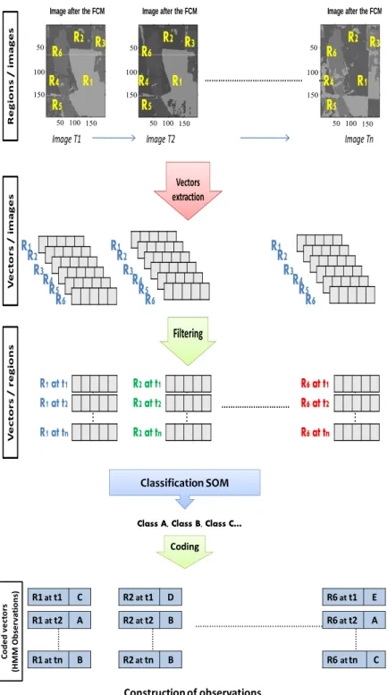
The feature vectors obtained are continuous and they can be quantified using a dictionary coding. The alterna-tive is to include densities of continuous observations in the model using a continuous HMM. But the large num-ber of parameters to be determined is a serious drawback of the model. Feature vectors are thus discretized using a Kohonen network [21]. This allows obtaining a dozen possible observations. Some of these observations serve as input for the HMM training phase. The choice is pro-portional to the surface of each class (see Figure 1).

The obtained data are then used in a hidden Markov chain to model the variation of the tracked object. A first order stationary hidden Markov model corresponds to two stochastic processes: one is a homogeneous Markov chain and the second depends on the first process.

Let be H 



h1, , hp



the set of P hidden states of

the system. Let S



S1, , ST



be a T-uple of random

(4)

R1

R2

R4

R3

R5

R6

R1

R2

R4

R3

R5

R6

R1

R2

R4

R3

R5

R6

Image T1 Image T2 Image Tn

………..…

R1

R2

R3

R4

R5

R6

R1

R2

R3

R4

R5

R6

R1

R2

R3

R4

R5

R6

…… …… R1 at t1 R1 at t2 R1 at tn …… …… R2 at t1 R2 at t2 R2 at tn

………

…… …… R6 at t1 R6 at t2 R6 at tn Filtering Vectors extraction Ve c t o r s / i m a g e s Re g ions / i m a g e s Ve c t o r s / r e g io n s

Image after the FCM Image after the FCM Image after the FCM

100 150 50 100 150 50 50 100 150 50 100 150 50 100 150 50 100 150 ………..……….. ………… ………… Coding Classification SOM

Class A, Class B, Class C…

………… R1att1 C R1att2 A R1attn B R2att1 D R2att2 B R2attn B R6att1 E R6att2 A R6attn C Co d e d v e cto rs (H M M Ob se rv at io n s) Construction of observations

Figure 1. Extraction and selection of training data.

variables defined on S. Let O



o1, , oq



be the set of P S

 

1 si

Q symbols that can be emitted by the system. Let

 the probabilities of transiting between two states:



1, , T



V  v  v be a T-uple of random variables defined



t j t1 i



P S s S s

on V. A hidden Markov model is then defined by the following probabilities:

 the probabilities of emitting a particular symbol for a particular state:

 the probabilities of starting the sequence with a par-ticular state:

(5)



t j t i



P V v S s

If the HMM is a first order stationary hidden Markov model then many simplifications can be done. Let:

 

i ₁ i p   with i P S



t si



 

i j, _{1 ,}_{i j p} A a _ _ with ai j, P S



t s Sj t1si



,

 



i



1 i p,1 j q B b j _{ } _{ } with b ji

 

P V



tv Sj t si



A first order stationary hidden Markov model  is then completely defined by the triple (A,B,∏). In the following, we will consider the notation  = (A,B,∏) and we note HMM a first order stationary.

We note



₁, ,



T a hidden state se-

T

Q q  q S

quence and



₁, ,



T an observed sequence

T O o  o V

of symbols. The probability that a state sequence Q and an observed sequence of symbols O occurs given a HMM  is



V O S, Q



. Probability dependencies allow to write:



,





, ,





P V O S Q  P V O S Q  P S Q 



With



, ,



1



T t t t t t P V O S Q  



_ P V o S q



and



 



1





1 1 1 1 1 , T t t t t t P S Q P S q   P S_ q_ S q      



 

From a HMM , a state sequence Q and an observed sequence of symbols O, we can compute the adequacy between the model  and the two sequences Q and O. For so, we need to compute the probability



,



P V O SQ . When the state sequence is unknown, it is possible to compute the likelihood of the observed sequence O given a model  by evaluating the probability:







,



Q S P V O P V O S Q   



 

When manipulating hidden Markov models, we commonly need to solve three kind of problems (for a given HMM ) :

 computing the likelihood,



O



 determining the state sequence _Q*_{that is the most} likely followed to emit the observed sequence O: the state sequence _Q*_{defined by the following equation} is efficiently computed by the Viterbi algorithm with a complexity of _{O p T}

 

2 _;





* _{arg max} _, T Q s Q  _ P VO S Q 

 Adjusting one or many HMMs from one or many observed sequences when the number of hidden state in HMMs is known: training can be viewed as a constrained optimization problem for which we try to maximize some criterion. There exist many criteria used for HMMs training [8]. When considering the maximization of the likelihood, we search a HMM

*

 satisfying the equation





* _{arg max} _{P V} _O

 

   

Up to now, there is no general solution to this problem but algorithms, such as the Baum-Welch algorithm [22] which is an iterative re-estimation which counted the number of times each state, each transition and each symbol was attached to the statements used in all sequences. We can also use the gradient descent [23] to improve an initial solution. Training algorithm for HMMs are iterative methods such that when iterating the algorithm, only a local optimum of the criterion can be found. This article attempts to show that it is reasonable to adopt a new pol- icy of learning so that the time series of satellite images provide a good prediction of space-time events.

Note that change detection may be of different types of origin and of varying lengths, which allows distinguish- ing different families of applications:

 Monitoring of land use, which corresponds to the characterization of the development of vegetative tis- sue, or the detection of seasonal changes in vegetation;

 The management of natural resources, which corresponds to the characterization of urban development, monitoring of deforestation...

 Mapping of damages, which corresponds to the loca- tion of the damages caused by natural disasters e.g. a volcanic eruption, a tsunami, an earthquake, a flood. Thus the hidden states of our model change depending on the application domain. Let consider the database system already constructed from phase 1 and containing a set V of data vectors describing each region in the study area at a time t:

P V   , of an observed sequence O given a model : this problem is efficiently solved by the Forward algorithm or by the Backward algorithm with a complexity of _{O p T}

 

2 [22];



1at ,1 2 at , ,1 m at ; ;1 1at ,n 2 at , ,n m at



V  R t R t  R t  R t R t  R t_n

(6)

tors previously calculated:









Class , vector i, , ,Class , vector i,

C_ A  X   Z  Y  _

The use of hidden Markov model requires a series of observations already calculate O: O



X1, , Xn



m

Y

and a set of hidden states , which vary with field of application.



1

, ,

E Y 

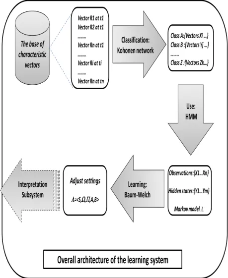
To adjust the parameters of HMM, we apply the Baum-Welch training. This allows for a transition matrix and an emission matrix to be computed (see Figure 2).

Phase 3:

Now that the HMM is known, we used its structure to either predict or decode events: given a HMM λ and o a sequence of observations, we seek to calculate the prob- ability of this sequence o with the HMM λ, i.e. with what probability the HMM generates the sequence o. This value is denoted by P(O=o, λ): this probability is effec- tively determined by the Forward or Backward algorithm. For this we developed a tool dedicated to the

evaluation to calculate the probability of a particular sequence to predict the end of spatiotemporal changes. Recognition involves finding the most likely sequence of hidden states that led to the generation of an output observed sequence. We then measure the recognition accuracy for each region, which is the percentage of events recognized at each time t relative to the total number of events in each region.

3. Experimentation

To validate our methodology, we conducted two applications. The first is generic based on SPOT images and the second is specific to the change in vegetation and uses a vegetation index in terms of variation and speed variation on Landsat images.

Overall architecture of the learning system

The base of

characteristic

vectors

VectorR1 at t1 VectorR2 at t1 …….. VectorRn at t1 …….. VectorRi at ti …….. VectorRn at tn

Classification:

Kohonen network

Class A:{Vectors Xi …} Class B :{VectorsYj …} …….. Class Z :{VectorsZk…}

Use:

HMM

Observations:{X1…Xn} Hiddenstates:{Y1…Ym} Markov model 

Learning:

Baum-Welch

Adjust settings

=<S,,,A,B>

Interpretation

Subsystem

(7)

3.1. First Experiment

The methodology described in the previous section is implemented using Matlab programming language, MS-Excel spreadsheet, free software for processing and image analysis: Multispec (normalization of multispec- tral satellite images), Image Analyzer (principal component analysis), UTHSCSA ImageTool (used to extract feature vectors of each region and to record in the learning database) and TANAGRA (used to classify and quantify all feature vectors using Kohonen maps). We tested our methodology on a sample of four sequences of time series of satellite images of Gueguen ADAM project in 2007 [24]. The image acquisition was daily for a period of 10 months, from October 2000 to July 2001 by Spot 1, 2 and 4 and concerns the area located in the Iflov departement at the East of Bucharest in Romania. Each series consists of 10 images of size 200 × 200. These sequences exhibit some phenomena that can be observed in the series. The first one is the harvesting of a field that

is the human activity most observable sky. The second shows the evolution of the forest in autumn. The third is the maturation of a field of rapeseed which appears in white. Finally, the fourth shows a changing river.

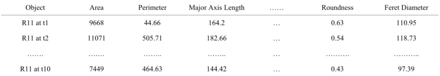
We began by analyzing each image time series to extract feature vectors of each region such as area, cen- troid, compactness, and save them in the learning data-base (see Table 1).

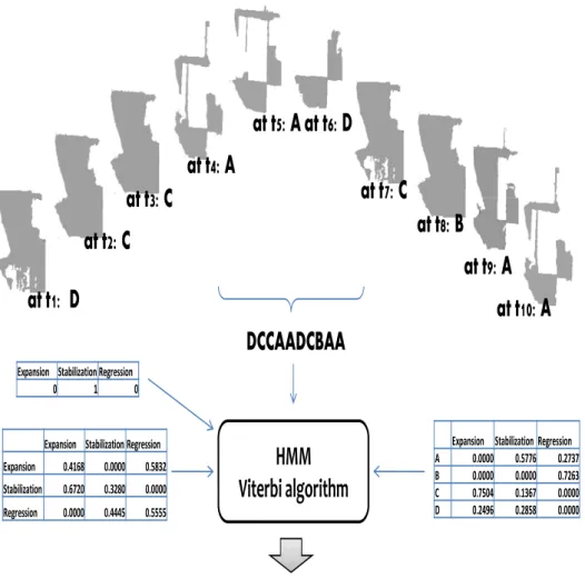
All these vectors were classified using Kohonen maps using data mining software TANAGRA. Thereafter each vector was identified by a code representing the class. Finally, our system tried to learn a HMM for each time series of satellite images from sequences of observations, when we set in the learning database the number of hid- den states, (i.e. a state for each type of spatiotemporal event), the transition matrix, the emission matrix and initial probabilities of departure. Once learning is com- pleted, we interpreted spatiotemporal events on regions of interest based on HMM. Figure 3 shows an example

HMM

Viterbi algorithm

Expansion Stabilization Regression

A 0.0000 0.5776 0.2737

B 0.0000 0.0000 0.7263

C 0.7504 0.1367 0.0000

D 0.2496 0.2858 0.0000

0 1 0

Expansion 0.4168 0.0000 0.5832 Stabilization 0.6720 0.3280 0.0000 Regression 0.0000 0.4445 0.5555

at t1: D

at t2: C

at t3: C

at t4: A

at t5: A

at t7: C

at t6: D

at t8: B

at t9: A

at t10: A

DCCAADCBAA

at T1: Stabilization, at T2: Expansion, at T3: Stabilization, at T4: Regression, at T5: Regression,

at T6: Regression, at T7: Expansion, at T8: Expansion, at T9: Regression and at T10: Regression.

(8)

Table 1. Some feature vectors of region R11 (the harvesting of a field) of the first sequence.

Object Area Perimeter Major Axis Length …… Roundness Feret Diameter

R11 at t1 9668 44.66 164.2 … 0.63 110.95

R11 at t2 11071 505.71 182.66 … 0.54 118.73

……. ….… …….. …….. … ………. ………..

R11 at t10 7449 464.63 144.42 … 0.43 97.39

of spatiotemporal analysis for a region that represents the harvest of a field, the recognition of different events (Stabilization (S), Expansion (E) and Regression (R) that led to the generation of the output data “DCCAAD CBAA” resolved with the Viterbi algorithm based on the training set containing previously constructed the transition matrix, the emission the matrix and probabilities of departure. ABCD was obtained by Kohonen network (see

Figure 2). This classification depends on descriptors

value for each region.

We can use interpretation system to predict the most likely event to a future date. For example, we want to re- cognize the most probable event at t = 11 and we al- ready know the series of events for t = 10. For example the sequence of observations “DACCCDABAD” creates a series of events “SRREEERRSE”, so we must calculate the probability of observing the sequences

“DACCCDABADA”, “DACCCDABADB”,

“DACCCDABADC” and “DACCCDABADD”. We then distinguish the set of observations that most likely occurs and therefore we can predict the event date t = 11 using the recognition task in our system of interpretation.

We present below (Table 2) the results of experiment- al tests. To specify each level of interpretation of events spatiotemporal length 10%, we present the rate and num- ber of corresponding regions. Table 2 shows examples of spatiotemporal analysis of some regions and their recog- nition accuracies. Tables 3 and 4 present the results of recognition and forecasting.

Note that using the evaluation function of our system, we can predict the state of the region. For example, class C is the most likely observation at t = 11 of the region R11 including the log of the probability of observing the corresponding sequence is “−17.4511”, and then we can estimate that the state provided the region R11 to t = 11 is the “stabilization”.

3.2. Second Experiment

The second application involved the analysis and monitoring changes in vegetation. We began by defining the various states the forest can be in. These states were defined relative to the change in forest area. The intervene- tion of an expert for the definition of these states is essential. But for operational reasons for implementation, we define the following states (see Figure 4):

Table 2. Experimental results. Accuracy of interpretation

of events Rate regions Number of regions

90% ≤ p ≤ 100% 15.625% 5 80% < p < 90% 28.125% 9 70% < p ≤ 80% 31.25% 10 60% < p ≤ 70% 9.375% 3 50% < p ≤ 60% 6.25% 2 40% < p ≤ 50% 6.25% 2 30% < p ≤ 40% 3.125% 1 20% < p ≤ 30% 0% 0 10% < p ≤ 20% 0% 0 0% < p ≤ 10% 0% 0 0% 0% 0 100% 32

Table 3. Example of results of recognition.

Time series Type analysis Precision

Serie n 1 Observation of a field crop 100%

Serie n 2 Changes in forest 70%

Serie n 3 Maturation of a field of rapeseed 80%

Serie n 4 Changes in river 90%

Table 4. Example of forecasting results of region R11 of the first sequence.

An expected observation o11 Probabilities of E11

Expansion 0.0000 Stabilisation 0.6281 A Regression 0.3719 Expansion 0.0000 Stabilisation 0.0000 B Regression 1.0000 Expansion 0.0000 Stabilisation 1.0000 C Regression 0.0000 Expansion 0.0000 Stabilisation 1.0000 D Regression 0.0000

(9)

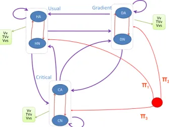
CA DN HN Vv TVv Vvs π1 π2 π3 HA DA CN Usual Critical Gradient Vv TVv Vvs Vv TVv Vvs

Figure 4. Model for monitoring changes in vegetation.  Usual (H) is the state of the forest when its surface is

in the range of 100% and 75% of the initial surface.  Gradient (D) is the state of the forest when its surface

becomes in the range of 75% and 60% of the initial surface

 Critical (C) is the state of the forest when the surface becomes less than 60% of the initial surface.

Note: the initial surface was defined by the forest area corresponding to the first image in the chronological order of the series. This surface is updated if we met in the series of images a larger area.

Each of these three states can have two different instances of speed variation of the surface. This speed was defined by the variation of the surface to the moment chosen from the surface to the moment before. We defined the following two instances:

 Normal (N) when the variation is less than 10% of the surface vegetation at the previous moment.

 Illness (M): When this variation is greater than 10% of the surface vegetation at the previous moment. In Figure 4 Vv, TVv and Vvs descriptors were respec- tively surface variation, vegetation rate change and healthy vegetation variation. The oriented arcs connecting the different states represent transitions from one state to another, this transitions can occur from one of two instances belonging to this state. The outgoing arrows represent each state emissions or comments made by this state and summarized by the descriptors change.

Note: The different thresholds for switching from one state to another (75% and 60%) and to move from one jurisdiction to another (10%) are chosen in an empirical way, so it was domain expert landlines.

We used a series of Landsat images from different regions, whose shape and surface randomly and continu- ously changed. For this, we created 15 time series each with ten images each two months between avril 2008 and march 2010. These series formed the sequence learning model and represent the area of North Africa (Tunisia,

Algeria and Egypt). At this stage, we should extract the region of interest in each image of the 15 time series to detect the change from one image to another, then to calculate the descriptors of variation. For this, we choose vegetation indices to be used to discriminate forest from the rest of the scene. The first index was the NDVI (Normalized Difference Vegetation Index) [25]. The index is strongly correlated with the chlorophyll activity of the vegetation, and is used to quickly and simply identify plant surfaces. The NDVI is typically 0.3 to 0.8 for bare soil and dense vegetation. It was therefore essential to set a threshold for the NDVI (0.4 used in literature [26]); the pixels with a value above this threshold were classified as vegetation. The remaining pixels were considered as the rest of the scene. The second index was the RVI (Ra- tio Vegetation Index) [25]. This index highlighted areas where vegetation was under stress, or not healthy, and sharpens between vegetation and soil. The overall RVI varies from 1 for bare floors to over 20 for dense vegetation. It is also essential to set a threshold for the RVI (equal to the average of RVI for all the pixels of the region), the pixels with a value above this threshold will be classified as healthy vegetation, and the rest will be considered unhealthy vegetation. We varied the threshold but it did not give conclusive results because of certain values (which are close to 0.4), we no longer distinguish between bare soil and vegetation. The descriptors calcu-lated from sequences of images were considered as the observations of a HMM. From these observations, was possible to determine the hidden states associated with them. This was done using rules like: IF “descriptor1 belongs to interval-X” AND “descriptor 2 belongs to interval-Y” THEN “state-Z”. The different intervals and states were defined based on thresholds already set. Ob- servations and corresponding hidden states were used as training data model. This training used Baum-Welch algorithm. This practice considered the continuous emission and thus provided “a probability distribution of generation according to a normal” in addition to the transition matrix between states A and the vector of initial probabilities Pi. In this HMM, the number of states is six because we have three hidden states (usual, gradient and critical) each one is composed by two instances (normal and illness).

The Probability of First Visit states: Pi = (0.4 0 0.1 0.2 0 0.3)

The matrix of transition probabilities between states: 0.71 0.08 0.08 0.09 0 0.02 0.62 0.37 0 0 0 0 0.36 0.09 0.27 0 0.18 0.09 0.36 0.18 0 0.36 0.09 0 0 0.25 0 0.25 0 0.5 0.18 0 0.27 0.09 0.09 0.36 A                     

(10)

To test the robustness and reliability of the model after learning, we used the model to generate the correct path to a given observation randomly selected. This was done using the Viterbi algorithm. Then, we determined the actual path corresponding to the same observation using the rules defined above. Finally, we compared both re-sults to calculate the error of the model.

Let the observation test defined by its descriptors: Observation test = [100 48.17 93.51 59.9 90.18 77.71 68.78 100 69.18 100 41.85 75.37 71.12 61.63 86.04 53.78 89.88 89.12; 0 51.83 0 35.95 0 13.83 11.48 0 30.82 0 58.15 0 5.631 13.35 0 37.5 0 0.8397]

The corresponding path generated by the model Viterbi path: [1 6 1 6 1 4 4 1 6 1 6 3 3 6 1 6 1 1] The actual path calculated by the Rules

Real path: [1 6 1 6 1 2 4 1 4 1 6 1 3 4 1 6 1 1]

The error was computed for eleven different observations; and we obtained a mean error of 8.38%. We noted that the error happened in different locations. These results show the efficiency of our system and indicate that NDVI can provide a useful index of vegetation variability.

The final step was to operate the predictive power of Markov models in general, and especially that of our model. Indeed, knowing the current state of the object track- ing “a forest”, and indicating to the system after how long we want to predict the condition of the forest, the system will give us the probabilities of being in each of the six states previously defined.

Example of current state of a forest gradient-normal (DN), corresponding state vector is [0 0 1 0 0 0]. After a period, probability vector of states becomes [0.364 0.09 0 0.273 0.182 0.09]. Note that a period is defined by time incurred between two successive acquisitions of satellite images constructing time series used for model training. For example, 0.364 means that we will translate to the state one with a probability of 36.4%.

4. Conclusions

The work of interpretation is complicated when analyz-ing changes from a series of satellite images spaced in time. It would be interesting to have one (or several) model(s) making the link between observations and real- ity for a specific purpose, and that even when observations are incomplete and/or inaccurate. In addition, to interpret the formal results and simply to explain to non- specialists, these results should be presented in sum- mary form. In this paper, we presented an approach that involves applying a number of pre-processing satellite images. We then built a hidden Markov model whose parameters were estimated by learning. Finally, we moved to the phase of interpretation, evaluation and forecasting. Our approach is validated by two experiences.

The results of the first experiment were quite accept- able. Indeed, 75% of events have been recognized with at

least an accuracy of 70% and 15.625% of events have been interpreted with an accuracy of 100%. For the second experiment, the evaluation of the robustness and reliability of the model provided satisfactory results with a reasonable error rate. Therefore, the methodology presented in this study is promising.

It provides a good prediction of spatiotemporal changes in conjunction with the monitoring of the latter. Besides, it is transferable to multiple applications such as monitoring and management of natural resources, dynamic monitoring of land use, risk assessment, mapping of da- mage, assessment of urban expansion, updating of to- pographic maps, etc. The model can be improved by in- corporating knowledge of an expert in the field of application.

Several researches and developments emerge from this work. The integration of technical change detection subsystem in the learning and assess the effect of this im- provement on system performance. It will also be interesting to extend our approach to spatio-temporal opera- tion of other models such as pairwise or triplets Markov chains.

REFERENCES

[1] J. Rodriguez, F. Vos and R. Below, “Annual Disaster Statistical Review 2008: The Numbers and Trends,” Cen- tre for Research on the Epidemiology of Disasters, 2009, pp. 1-33.

[2] A. Singh, “Digital Change Detection Techniques Using Remotely-Sensed Data,” International Journal of Remote

Sensing, Vol. 10, No. 6, 1989, pp. 989-1003. doi:10.1080/01431168908903939

[3] D. Lu, P. Mausel, E. Brondizio and E. Moran, “Change Detection Techniques,” International Journal of Remote

Sensing, Vol. 25, No. 12, 2004, pp. 2365-2407. doi:10.1080/0143116031000139863

[4] P. Coppin, I. K. Jonckheere, B. Nackaerts and B. Muys, “Digital Change Detection Methods in Ecosystem Moni-toring: A Review,” International Journal of Remote

Sensing, Vol. 25, No. 9, 2004, pp. 1565-1596.

doi:10.1080/0143116031000101675

[5] M. Lazri, S. Ameur and B. Haddad, “Analyse de Données de Précipitations par Approche Markovienne,” Larhyss

Journal, Vol. 6, 2007, pp. 7-20.

[6] J. F. Mari and F. Le Ber, “Temporal and Spatial Data Mining with Second-Order Hidden Markov Models,” Soft

Computing, Vol. 10, No. 5, 2006, pp. 406-414. doi:10.1007/s00500-005-0501-0

[7] H. Sagan, “Space-Filling Curves,” Springer-Verlag, Ber- lin, 1994.

[8] S. Aupetit, M. Slimane and N. Monmarche, “Utilisation des Chaînes de Markov Cachées à Substitution de Sym- boles Pour l’Apprentissage et la Reconnaissance Ro- buste d’Images,” 2nd Proceeding of MAJECSTIC, 13-15 October 2004, Calais, pp. 245-269.

(11)

[9] L. Aurdal, R.B. Huseby, D. Vikhamar, L. Eikvil and A. Solberg, “Use of Hidden Markov Models and Phenology for Multitemporal Satellite Image Classification: Applica- tions to Mountain Vegetation Classification,” 3rd Inter-

national Workshop on the Analysis of Multi-Temporal Remote Sensing Images, Biloxi, 16-18 May 2005, pp. 220-224.

[10] W. Pieczynski, “Triplet Markov Chains and Image Seg- mentation,” Draft of Chapter 4 in Inverse Problems in Vi-sion and 3D Tomography, Wiley, Hoboken, 2010. [11] W. Pieczynski, “Pairwise Markov Chains,” IEEE Trans-

actions on Pattern Analysis and Machine Intelligence,

Vol. 25, No. 5, 2003, pp. 634-639. doi:10.1109/TPAMI.2003.1195998

[12] W. Pieczynski, C. Hulard and T. Veit, “Triplet Markov Chains in Hidden Signal Restoration,” Proceedings of

SPIE 4885, Image and Signal Processing for Remote Sensing VIII, Crete, 22-27 September 2002, pp. 58-68.

[13] C. Carincotte, S. Derrode and S. Bourennane, “Unsuper- vised Change Detection non SAR Images Using Fuzzy Hidden Markov Chains,” IEEE Transactions on Geo-

sciences and Remote Sensing, Vol. 44, No. 2, 2005, pp.

432-441.

[14] S. Derrode and W. Pieczynski, “Signal and Image Seg- mentation Using Pairwise Markov Chains,” IEEE

Trans-actions on Signal Processing, Vol. 52, No. 9, 2004, pp.

2477-2489. doi:10.1109/TSP.2004.832015

[15] A. B. Wijanarto, “Application of Markov Change Detec- tion Technique for Detecting Landsat ETM Derived Land Cover Change over Banten Bay,” Jurnal Ilmiah

Geo-matika, Vol. 12, No. 1, 2006, pp. 11-21.

[16] C. Lacoste, X. Descombes, J. Zerubia and N. Baghdadi, “Extraction Automatique des Réseaux Linéiques à Partir d’Images Satellitaires et Aériennes par Processus Markov Objet,” Bulletin de la SFPT, Vol. 170, 2003, pp. 13-22. [17] C. Song, “Spectral Mixture Analysis for Subpixel Vege-

tation Fractions in the Urban Inveronment: How to In- corporate Endmember Variability?” Remote Sensing of

Inveronment, Vol. 95, No. 2, 2005, pp. 248-263. doi:10.1016/j.rse.2005.01.002

[18] V. Michel, “Analyse des Données,” 4th Edition, Eco- nomica, Paris, 1997.

[19] B.-Y. Kang, D.-W. Kim and Q. Li, “Spatial Homogene- ity-Based Fuzzy c-Means Algorithm for Image Segmen- tation,” Proceedings of Second International Conference

on Fuzzy Systems and Knowledge Discovery, Changsha,

27-29 August 2005, Part I.

[20] D. L. Phum, “Spatial Models for Fuzzy Clustering,”

Computer Vision and Image Understanding, Vol. 84, No.

2, 2001, pp. 285-297. doi:10.1006/cviu.2001.0951 [21] T. Kohonen, “Self-Organizing Maps,” Springer-Verlag,

Berlin, 1995.

[22] L. R. Rabiner, “A Tutorial on Hidden Markov Models and Selected Applications in Speech Recognition,” Pro-

ceeding of the IEEE, Vol. 77, No. 2, 1989, pp. 257-286. doi:10.1109/5.18626

[23] S. Kapadia, “Discriminative Training of Hidden Markov Models,” Ph.D. Dissertation, Downing College-Univer- sity of Cambridge, Cambridge, 1998.

[24] L. Gueguen, “Extraction d’Information et Compression Conjointes des Séries Temporelles d’Images Satelli- taires,” Ph.D. Dissertation, l’École Nationale Supérieure des Télécommunications de Paris, Paris, 2007.

[25] J. G. Lyon, D. Yuan, R. S. Lunetta and C. D. Elvidge, “A Change Detection Experiment Using Vegetation Indices,”

Photogrammetric Engineering and Remote Sensing, Vol.

64, 1998, pp. 143-150.

[26] B. M. Ranga, G. H. Forrest, J. S. Piers and L. M. Alex- ander, “The Interpretation of Spectral Vegetation In- dexes,” IEEE Transactions on Geosiences and Remote