Available transfer capability for electric power markets : a critical appraisal

Available Transfer Capability for Electric Power Markets:

A Critical Appraisal

by

Ahmed

D. Alumran

Submitted to the Department of Electrical Engineering and Computer Science in Partial Fulfillment of the Requirements for the Degrees of

Bachelor of Science in Electrical Science and Engineering

and Master of Engineering in Electrical Engineering and Computer Science at the

MASSACHUSETTS INSTITUTE OF TECHNOLOGY June 1998

@

A uthor... ... ...

Sar

' Electrical Engineering and Computer Science May 22, 1998

C ertified by ... . .. .. .. ... ... .... ... ... ...

/

Senior Research Scientist

Accepted by ... .. ... •.... ... t;" . thur C. Smith Chairman, Department Committee on Theses MASSACHUSETTS INSTITUi L

OF TECHNO -:( OGY

JUL

141998

Available Transfer Capability for Electric Power Markets:

A Critical Appraisal

by

Ahmed D. Alumran

Submitted to the

Department of Electrical Engineering and Computer Science May 22, 1998

In Partial Fulfillment of the Requirements for the Degrees of Bachelor of Science in Electrical Science and Engineering

and Master of Engineering in Electrical Engineering and Computer Science

Abstract

This thesis concerns the physical limitations of an electric transmission network serv-ing newly evolvserv-ing energy markets. The capability of the network is measured in terms of so-called available transfer capability (ATC), a term recently introduced. In this thesis various definitions of ATC are evaluated in order to illustrate its multi-dimensional character. This study is motivated by our perceived need to more care-fully measure the physical limitations of the network as a function of the energy market structure in place. The definition presently adopted by the industry is well suited only for centralized power exchange. To show this, we first review the definition of ATC as introduced by the North American Electric Reliability Council (NERC). After a brief discussion of some of the conceptual issues, several recently proposed definitions of ATC are presented and illustrated using a hypothetical 3 bus power net-work. These alternative definitions include the system transmission capacity (STC), load bus transmission capacity (LBTC), and bilateral transmission capacity (BITC). Secondly, the ATC definitions are evaluated on a 5 bus and a 39 bus electric power network. Both a linear dc load flow model and a nonlinear coupled load flow model are employed for calculations. This is made possible by the development of a com-puter simulation for each model that executes an optimal power flow algorithm to evaluate ATC definitions. The results show a strong dependence of the transfer capa-bility available to market participants upon the definition of ATC being applied, with cases where the STC is not meaningful in the context of bilateral transfers. Finally, it is shown that ATC is directly related to line flow constraints, it varies with slack bus choice, and it increases as the minimum load bus voltages are allowed to drop relative to the generator bus voltages. It is also indicated that STC is more sensitive to changing these system parameters than other ATC definitions.

Thesis Supervisor: Dr. Marija Ilid Title: Senior Research Scientist

Acknowledgements

To my Father, Mother, and Sister for their love and support

and to my Grandfather and Grandmother for their caring and wisdom

Contents

1 Introduction 8

1.1 Historical Perspective ... 8

1.2 Thesis Objectives ... 9

2 Background 10 2.1 Industry definition of ATC ... ... 10

2.2 Purpose of ATC and Challenges ... .. 11

3 Alternative Definitions of ATC 14 3.1 Key Points and Assumptions ... 14

3.2 System Transmission Capacity (STC) . ... 15

3.3 Bus Transmission Capacity (LBTC / GBTC) . ... 15

3.4 Bilateral Transmission Capacity (BITC) . ... 17

3.5 3 Bus Network Example ... 17

4 Linearized Model-Based ATC Calculations 22 4.1 Method of Calculation ... 22

4.2 DC Load Flow ... 23

4.3 5 Bus Network ... ... 26

4.4 39 Bus Network ... ... 29

5 Non-Linear Model-Based ATC Calculations 30 5.1 OPF with Coupled Load Flow Equations . ... . . 30

5.3 39 Bus Network ...

6 Changing System Parameters 34

6.1 Flow Constraints ... 34

6.2 Dependence on the Choice of a Slack Bus . ... 35

6.3 Voltage Constraints ... ... 37

7 Conclusions 39

A Basic Load Flow Problem 41

B Network Parameters for the 5 and 39 Bus Networks 43

C Optimal Power Flow Formulation 45

D Voltage Constraints and ATC 47

List of Figures

2-1 Adding a Path of Transmission to a Subnetwork . . . . 2-2 Maximum Line Flows of the Subnetwork Example . . . . 3-1 LBTC & GBTC as Bounds for an Incremental Power Interchange 3-2 3 Bus Network Example for Calculating ATC

3-3 Incremental Line Flows for Network 1 of the 3-4 Incremental Line Flows for Network 2 of the

. . . . . 18 3 Bus Example 3 Bus Example 4-1 5 Bus Network ... 4-2 39 Bus Network ... 6-1 6-2 6-3

Variation of STC with Voltage Constraints . . . . Variation of LBTC4 with Voltage Constraints . . . .

Variation of BITC42 with Voltage Constraints . . . .

... . 26

. .. . 29

. . . . 37

. . . . 38

. . . . 38

List of Tables

3.1 ATC values for the 3 Bus Example ... 21

4.1 Nominal & Final Injections for the Linear 5 Bus Network ... 26

4.2 Nominal & Final Line Flows for the Linear 5 Bus Network ... 27

4.3 Incemental Injections at the STC of the Linear 5 Bus Network . . .. 27

4.4 ATC Definitions Evaluated with Linear Model on the 5 Bus Network 28 4.5 ATC Definitions Evaluated with Linear Model on the 39 Bus Network 29 5.1 Nominal & Final Conditions for the Nonlinear 5 Bus Network . . . . 31

5.2 Nominal & Final Line Flows for the Nonlinear 5 Bus Network . . . . 31

5.3 Incemental Injections at the STC of the Nonlinear 5 Bus Network . . 32

5.4 ATC Definitions Evaluated with Nonlinear Model on the 5 Bus Network 32 5.5 ATC Definitions Evaluated with Non-linear Model on the 39 Bus Network 33 6.1 Evaluating ATC definitions with Different Flow Constraints .... . 34

6.2 The Effect of Changing the Slack Bus on Yinitial . . . . . . 35

6.3 Evaluating ATC definitions with Different Slack Buses . ... 36

B.1 5 Bus Network Parameters ... ... 43

B.2 39 Bus Network Parameters ... 44 D.1 Data Points for Comparing Voltage Constraints with ATC Definitions 47

Chapter 1

Introduction

1.1

Historical Perspective

In 1992 the United States Congress developed the Federal Power Act, which has been interpreted by the Federal Energy Regulatory Commission (FERC) as a mandate to introduce open-access of transmission resources and generation competition to the electric power industry. In the following years, FERC issued a Notice of Proposed Rulemakings (NOPRs) that would hint at the direction FERC was headed and seek comment from industry. The result of this process occurred in 1996 when FERC issued Orders 8881 and 8892.

The commercial success of an open and competitive electric power market depends on accurate, up-to-date information about the capacity of the transmission network to accommodate power transfers requested by the market participants. This information has been labelled the ATC (available transfer capability) of a network, and it is posted on a system called OASIS. FERC has ordered that bulk electrical control areas must provide to market participants a commercially viable network transfer capability for the import, export, and through-put of energy.

The FERC has deferred the development of technical guidelines for both ATC and

1Promoting Utility Competition Through Open Access, Non-Discriminatory Transmission Service by Public Utilities; Recovery of Stranded Costs by Public Utilities and Transmitting Utilities

the OASIS to the North American Electric Reliability Council (NERC), an industry group that develops reliability standards and guides for the planning and operation of electric power systems in the United States and Canada. NERC has brought together the industry to establish a framework for defining ATC, and is leading a major effort on formulating key principles of ATC evaluation [2].

1.2

Thesis Objectives

In this thesis we review the definition of ATC as proposed by NERC as well as several recently introduced definitions, and evaluate these definitions in different scenarios. The goal is to show a multi-dimensional aspect of ATC through a series of illustrative calculations. We suggest that the definitions used directly depend on the energy market structure in place. Some concepts are more suited for centralized (poolco-like) markets, and others are more effective for facilitating bilateral energy markets.

Chapter 2

Background

2.1

Industry definition of ATC

Available transfer capability has been defined by NERC as the following [3]:

Available Transfer Capability (ATC) of a subnetwork within the U.S. intercon-nection is a measure of the transfer capability remaining in the physical trans-mission subnetwork for further commercial activity over and above already com-mitted uses. ATC is defined as the Total Transfer Capability (TTC), less the Transmission Reliability Margin (TRM), less the sum of existing transmission commitments and the Capacity Benefit Margin (CBM). Or put more simply,

ATC = TTC - TRM - CBM - Existing Transmission Commitments

The NERC definition of ATC depends on the following subset of definitions: Total Transfer Capability (TTC) is defined as the amount of electric power that

can be transferred over the interconnected transmission network in a reliable manner.

Transmission Reliability Margin (TRM) is the amount of transfer capability necessary to ensure that the interconnected transmission network is secure under a reasonable range of system conditions.

Capacity Benefit Margin (CBM) is the amount of transfer capability reserved by load serving entities to ensure access to generation from interconnected neigh-boring systems to meet generation reliability requirements.

2.2

Purpose of ATC and Challenges

The transmission network is no longer being used in the manner and to the extent that was planned when it was designed. Open access is generating a greater volume of transactions, higher frequency of violating transmission line constraints, and increas-ing number of reservations of transmission service. These effects have introduced a series of new challenges to industry participants, because transmission service is vital to the proper functioning of competitive electricity markets [4].

The purpose of calculating ATC and posting it on the OASIS is to further the open-access of the transmission system by providing a signal of its capability and availability to deliver energy. ATC should give parties interested in trading power usable and useful data about the extent to which they may inject or receive power from the network without violating technical operating constraints. The OASIS system makes the ATC for a region accessible to market participants through the Internet. Not only should this allow for a more efficient utilization of and planning for the transmission network, but more importantly, it should promote competitive bidding in the generation market.

The key challenge to more efficient utilization of the transmission network is the inability of a single ATC to adequately capture all the information necessary for each power transfer across a network. Firstly, since each power transfer on a network reduces the available transfer capability of other potential transfers, the ATC of a network must be continually updated. Secondly, the ATC of a power transfer on a subnetwork cannot be evaluated in isolation. In other words, information about all paths of transmission between the originating and destination buses of a power transfer must be taken into consideration for evaluating ATC. The importance of this last point can be illustrated through the simple 3 bus example shown in Figure 2-1.

In order for this example to conform with NERC's definition of ATC, it is necessary to define bus 1 and bus 3 respectively as the only generation and load bus on this subnetwork. The maximum line capacities correspond to transfers above some base level of operation and are the only system constraints. Also note that bus 2 does not

MAX 400 MAX 700 MAX 400 MAX 700 200

Figure 2-1: Adding a Path of Transmission to a Subnetwork participate in any power transfer.

On the left of Figure 2-1, it would be assumed without additional information that the ATC from bus 1 to bus 3 is 400, which is the minimum of the line capacities of linel-2 and line2_3. Although this would be correct if no alternative lines existed

between bus 1 and bus3, this is rarely the case in an interconnected transmission network. Adding linel-3 as in the right of Figure 2-1 changes the ATC to 300, as can

be seen from the characterization of this subnetwork's line flows in Figure 2-2.

900

0

S to100 200

500 900 MAX

Figure 2-2: Maximum Line Flows of the Subnetwork Example

Because power is not transmitted from point to point but distributed along all transmission lines, information about the entire interconnected network is necessary in order to properly calculate ATC. This can become prohibitive for very large scale networks if ATC has to be posted in real time.

Another challenge facing the usefulness of the currently used ATC definition is the inconsistency of methods for evaluating it in various parts of the United States [5]. ATC is currently posted as a single network number that measures the ability of the

interconnected electric power system to reliably transfer power from one subnetwork to another over all transmission lines interconnecting the subnetworks for specified line flows in these interconnecting lines. In a simple network, this form of ATC can be viewed as the maximum additional power, over some base condition, that can be received by all load buses from all generator buses according to some set of constraints. However, the problem with this view is that ATC is actually a multi-dimensional property of networks. The maximum transmission capacity available to the generators and loads of a network is not unique for every set of power transfers. What does the ATC of a transmission network, as defined by NERC, tell a generator about how much power it can transfer to a particular load? Although this view of ATC can be regarded as an index of how congested the network is at a particular time, it by no means presents an accurate estimate of the capacity available to individual bilateral or multilateral power transfers by market participants.

Chapter 3

Alternative Definitions of ATC

3.1

Key Points and Assumptions

A set of alternative definitions for ATC have been recently introduced [6] which account for different types of power transfers across the transmission network. These definitions are sufficiently general to be utilized for calculating ATC independent of industry structure or network topology. However, before presenting these definitions, several key points and assumptions about ATC should be mentioned.1

1. ATC is an extreme mode of operation of a power system, maximizing some measure of power transfer from generators to loads.

2. There is no unique way of representing ATC, as manifested by the plurality of definitions to be presented, though some definitions may be particularly useful. 3. It is necessary when defining ATC to enforce all steady-state and transient

operational and contingency conditions, or "security conditions."

4. Operating the transmission network at its transmission capacity does not gener-ally correspond to an economicgener-ally optimum level. The network is being pushed to some extreme state in order to maximize power transfers, not minimize costs. Any limits on operational costs should be included with the security conditions as constraints when defining and computing ATC.

5. ATC may vary over the seasons and according to the availability of equipment. There is increased uncertainty when quantifying it over longer time horizons,

1These are the actual points and assumptions made in the paper [6] that introduced the alterna-tive definitions of ATC.

and it may be necessary to expand the following definitions from their deter-ministic context.

3.2

System Transmission Capacity (STC)

The system transmission capacity (STC) is the maximum total incremental load2 above a normal point of operation that can be securely3 transmitted through a given network from the generation to the load buses. This STC is the conventional definition of ATC, where the security conditions incorporate all necessary constraints.4

It is important to note that there are no restrictions in this definition on individual generators or loads such as load uniformity or generation dispatch. These quantities are completely free to vary unless their individual ranges are constrained within the security conditions. STC is expressed as:

STC = max APd (3.1)

S

APd

ieLoads

where APdi is the incremental load at bus i, APd is the total system incremental load, and S indicates that this maximum lies within the security region.5

3.3

Bus Transmission Capacity (LBTC

/

GBTC)

The load bus transmission capacity (LBTC) is the maximum real power received at a given network bus, incremental above a given operating point, that can be securely transmitted through the network from all system generation buses.

The LBTCi defines the maximum possible incremental load that can be supplied

2_{A similar definition could have been proposed with total maximum generation, which would} differ by the system transmission losses.

3 "Securely" implies that all security conditions mentioned above are met.

4These constraints may incorporate the TRM, CBM, and existing transmission commitments discussed earlier.

5The concept of security regions is beyond the scope of this work. What is important is to realize that being within the security region implies that all security conditions are met

by the network to a particular bus i. No assumptions are made about where this power is generated, and all generators may vary within their individual limits of operation. However, all incremental loads are set to zero except for bus i. LBTC is expressed as:

LBTCi = max APdi (3.2)

s

A Pdj = 0;j:i

Analogously, a generation bus transmission capacity may be defined as the maxi-mum power that can be sent from a given bus to the all load buses. In general, LBTC and GBTC are not equal even if calculated at the same bus since, in a system with transmission limits, the ability of a bus to send and receive power may differ. GBTC is expressed as:

GBTCi = max APi (3.3)

S

APj = 0; j i

The LBTC and GBTC define upper bounds on the capacity of a given bus to receive or send power from or to other buses in the network regardless of the con-sequences that operation at this bound may have on the capacity to send or receive power at other network buses. Although it would not be normal to operate at these maxima due to the sharp reduction in the transmission capacity of other buses, these definitions do provide a measure of the extent to which a given bus may participate in power interchanges. For example, the LBTC and GBTC can serve as upper bounds on any potential incremental interchange from or into the network, as represented by

-LBTCi < APi < GBTCi

where APi is defined as the real power injection into bus i.

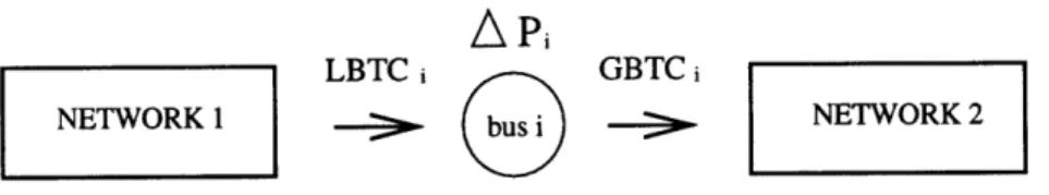
In the Figure 3-1, all incremental loads in Network 1 and all incremental gener-ators in Network 2 are set to zero. Thus, LBTCi and GBTCi give an indication of

A Pi

LBTC i GBTCi

NETWORK 1 bus i NETWORK 2

Figure 3-1: LBTC & GBTC as Bounds for an Incremental Power Interchange how much incremental generation APi, above the normal point of operation, can be provided by Network 1 to Network 2 through Bus i.

3.4

Bilateral Transmission Capacity (BITC)

The bilateral transmission capacity (BITC) is the maximum real power, incremental above a given operating point, that can be securely received at bus i from bus j. It is a special case of LBTC in which only one particular generator transmits power. As with the previous definitions, BITC is an extreme mode of operation that will limit the capacity of other buses to transfer power. Nevertheless, BITC provides an upper bound to limit potential bilateral transactions. BITC is expressed as:

BITCij = max APdi (3.4)

S APg k = 0; k

4

APdm = 0; m A i

The BITC could also have been defined in terms of the power sent from one bus to another. A natural extension of this definition is to represent multilateral exchanges between sets of load buses and generation buses rather than single pairs of buses.

3.5

3 Bus Network Example

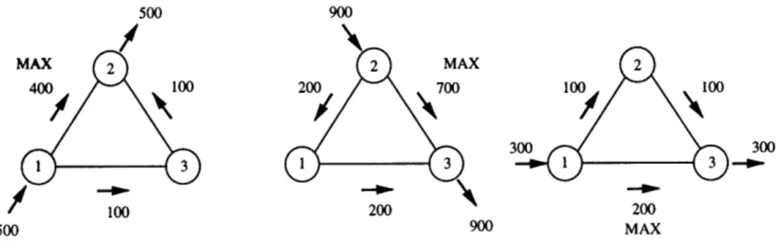
The following 3 bus network example is presented in order to illustrate how the alternative ATC definitions may be defined and calculated. The objective of this

example is to give a better sense of how, even in such a simple 3 bus scenario, ATC must be defined in terms of the underlying power transfers taking place.

20 MAX[75]1 G 80 60 4 5 I[50] NETWORK 2

80\

20

t

Figure 3-2: 3 Bus Network Example for Calculating ATC

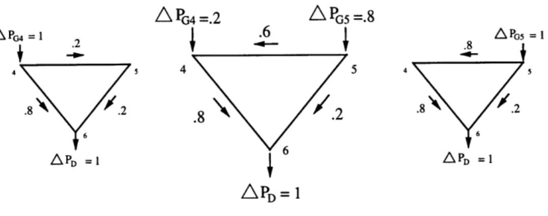
Networks 1 and 2 are almost identical except for the number of generators and loads. Figure 3-2 shows the maximum line capacities and the nominal power injections and flows for each network. In order to calculate a particular definition of ATC, it will be necessary to know how 1 unit of incremental power injected or received at a particular bus will flow through each network. This information is made available in the incremental line flow networks shown in Figure 3-3 and Figure 3-4. In each figure, superposition is used to combine the left and right networks to produce the central network where all buses participate in incremental power transfers.

APG= 1 APG1 APG =1 2 3 . PD3 = I APD3 = I IL PD2 = 1 A PD2=. 2 _{A PD} 3 =.8

Figure 3-3: Incremental Line Flows for Network 1 of the 3 Bus Example

MAX

2

I

3

SPG4 =.2 P5 =.8 APG4=1 , .6

I

Figure 3-4: Incremental Line Flows for Network 2 of the 3 Bus Example

The only security constraint in this simplified example will be that the maximum line capacities shown in Figure 3-2 are not exceeded. The maximum incremental injection or load for each combination of buses will be found by looking at the set of inequalities representing the flows on each line.

Nominal Line Flow + k x AP < Maximum Line Flow (3.5)

where nominal and maximum line flows are obtained from Figure 3-2, k (a constant representing the fraction of incremental injections flowing in each line) is obtained from the appropriate incremental line flow network in Figure 3-3 or Figure 3-4, and AP is solved for as the incremental power transfer being maximized.

From the alternative definitions of ATC presented earlier, STC is the maximum incremental power, beyond some nominal operating point, that can be received by all load buses from all generator buses while not violating any security constraints. Thus, STCNETWORK1 is the maximum APD = APD2 + APD3 that can be received by

buses 2 and 3 from the generator at bus 1 while Pij 5 1max (Pis) for all line flows.6 Using Equation 4, max (APD) can be found by solving:

80 + .8 x APD < 120

20 + .2 x APD 50

6_{Note that all networks in this example are lossless and thus APD = APG.}

60 + .6 x APD < 75

It can easily be seen that the third inequality is the limiting case, which means that

line2_3 is first to reach its capacity, and that STCNETWORK1 = 25. From the definition

of GBTC previously given, it should be noted that GBTC1 = STCNETWORK1 since

Network 1 has only one generator bus. 7

In order to calculate LBTC2, bus 3 is not allowed to receive any incremental

injection from bus 1 beyond the 80 units already being transfered at the nominal operating point. 8 The inequalities used to calculate max (APD2) are:

80 + .8 x APD2 < 120 20 + .2 x APD2 < 50

60 + .2 x APD2 < 75

The limiting case here is the first inequality, which means that linel-2 is first to

reach its capacity. Thus, LBTC2 = 50. Proceeding in a similar manner, it is found

that LBTC3 = 18.75 as line2-3 reaches its capacity. Furthermore, by the definitions

of BITC given earlier, BITC2-1 = LBTC2 and BITC3-1 = LBTC3. 9 The ATC

definitions for Network 2 can be calculated in the same way. The difference here is that there are two distinct values for GBTC and that STCNETWORK2 = LBTC6. 10

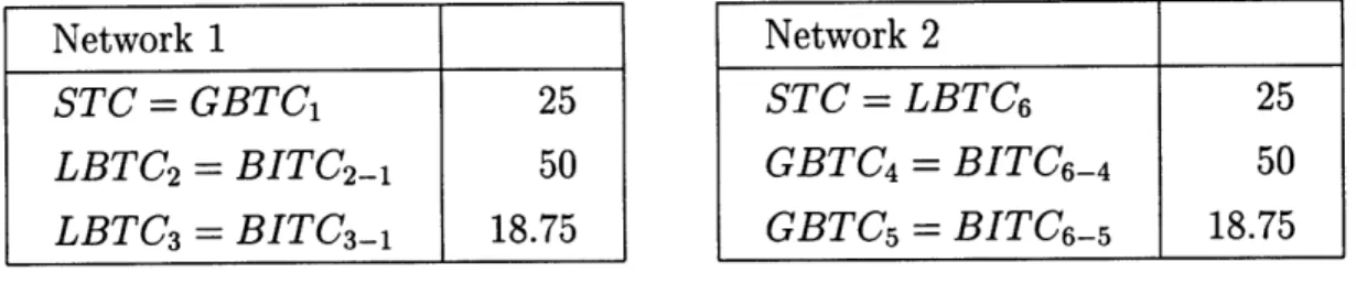
The ATC values for both Network 1 and 2 are summarized in Table 3.1.

It is apparent from the results obtained in this 3 bus example that the manner in which ATC is defined and calculated has a significant impact on the possibilities open to the buses on a network. For instance, bus 2 would be misled by judging the maximum power that could be received from Network 1 to be STC = 25, which is the conventional definition of ATC. In fact, as can be seen from the value of LBTC2 = 50,

bus 2 would be underestimating by a factor of 2. On the other hand, bus 3 would

7_{Another important condition is that the network is lossless. In general, GBTC is the special} case of an STC calculated from the generator buses. If losses exist, GBTC cannot be equal to the conventional STC which is calculated from the load buses.

8_{Once again, note that APD}

2 = APG because the network is lossless

'This is because there is only one generator bus in Network 1 from which all power at the load buses is received

Table 3.1: ATC values for the 3 Bus Example

overestimate the amount of power available from Network 1 by looking only at the STC, and could potentially cause damage to the network if a transfer of more than LBTC3 = 18.75 occurs.

Finally, the values of GBTC for Network 2 show that bus 4 is able to deliver more than twice what bus 5 can deliver to bus 6. If only the STC for Network 2 was available, bus 4 would not be able to take advantage of its favorable position on the network and profit from selling up to GBTC4 = 50 units of power to bus 6.

Conversely, bus 5 would be unaware that it is incapable of delivering more than a maximum of GBTC5 = 18.75 units of power.

Network 1 STC = GBTC1 25 LBTC2 = BITC2-1 50 LBTC3 = BITC3_1 18.75 Network 2 STC = LBTC6 25 GBTC4 = BITC6-4 50 GBTC5 = BITC6_5 18.75

Chapter 4

Linearized Model-Based ATC

Calculations

4.1

Method of Calculation

In order to evaluate ATC for larger networks, more involved methods of calculation are required. It is no longer feasible to calculate the incremental line flows for every combination of injections on a network and then solve an inequality for each line, as was done in the 3 bus example. For the 5 bus and 39 bus networks to be analyzed, computer simulations were used to perform the necessary calculations.

The preliminary data that is typically available about a network is the topology and parameters such as the resistance, reactance, and capacitance of each line. Nom-inal power injections are also specified at each bus, as well as the voltages at each generator bus.1 In more realistic networks, it also becomes necessary to define a slack bus, which is a generator bus that is used for the purpose of calculation and loss

compensation2

A simulation has been developed on Matlab for each model to be used for calcu-lating ATC. A linear dc load flow model and a non-linear coupled load flow model

'These specifications are explained in Appendix A. Note that generator bus voltages are not used in the linear model

have been chosen so that a comparison can be made of the resulting ATC values. Al-though each model has its own methodology, the maximization of incremental power

injection in both cases is treated as a constrained optimization problem.

4.2

DC Load Flow

The first model used is the dc load flow model [16], which provides approximate but simple relationships between generation and demand levels at the buses and real power flows through the lines of a network. The real power z12 flowing from bus 1 to

bus 2 along line i in a network and is given by3

Z12 = Gi[V2

-VV 2 cos (61 - 62)] + QiVV2sin(61 - 62) (4.1) Gi -=

Xi

R + X2

where V and 6 are the voltage and phase angle at a particular bus, and Ri and Xi are the line resistance and reactance.

The series of assumptions are made in the dc load flow model greatly simplify the calculations required to obtain the power flows through a network. Firstly, the phase angle difference between buses is assumed to be small in magnitude so that

COS (61 - 62) 1 (4.2)

sin

(61 -

)

(6 - 62)

Secondly, given that a per unit system is being used4, it is assumed that V1 1

and V2 0 1 so that Equation 4.1 reduces to5

Z12 = i(61 - 2) (4.3) 3 See Appendix A 4 See Appendix A. 5

Although a major drawback of this model is losing the ability to observe any changes in bus voltages or line losses, these assumptions are often used in actual utility operations and planning for transmission lines. The results thus obtained are highly useful for characterizing power flows and providing intuition about which lines will first reach their capacity when pushing a network to its extreme, as is done in all ATC calculations.

In order to proceed with how the dc load flow model solves the line flows as a function of network characteristics and bus injections, the following variables need to

be defined [16]:

NB: Number of buses NL: Number of lines

y: NB - 1 vector of bus injections (generation -demand) at all buses except the slack bus.

fl: NL x NL diagonal matrix of the reactances Di A: NL x (NB - 1) reduced network incidence matrix6 z: NL vector of line flows

6: NB - 1 vector of voltage angles at each bus except the slack bus where 6 = 0 7

Since the sum of all power entering a bus is zero,

y = AT z (4.4)

The matrix form of Equation 4.3 is

z = DA 6 (4.5)

Combining Equations 4.4 and 4.5 yields

y = AT A A (4.6)

6_{This is a matrix with 0, 1, -1 elements corresponding to network interconnections. The 5 bus}

example presented later in this chapter illustrates how it is constructed.

Solving for S yields

6 = (AT Q A)-' y

Substituting into Equation 4.5 yields

z = Hy (4.7)

H = QA(ATQA)- 1

H is called the transfer admittance matrix and is the essence of the dc load flow model since it combines any combination of a network's bus injections y to yield a vector of the line flows z.

Once the transfer admittance matrix has been calculated, the various definitions of ATC may be obtained using computer simulation to maximize the injections8 at all relevant buses without violating any line constraints. This procedure may be summarized as

max(Yinc); z = H (y + Yinc), z _ Zmax

where Yinc is a NB - 1 vector of incremental bus injections' and zmax is a NL vector of line constraints.10

8_{The incremental generation is maximized and the incremental load is minimized since it is}

negative

9_{This vector is all zeros except for a 1 at each generator bus and a -1 at each load bus that} is participating in incremental injections as required by the ATC definition being evaluated. For

example, if BITC1-2 was being evaluated, then yinc would be all zeros except for a -1 at bus 1 and

a 1 at bus 2.

10The only security condition that is applied in evaluating ATC is not violating any flow con-straints, except for the section in Chapter 6 where voltage constraints are also applied

4.3

5 Bus Network

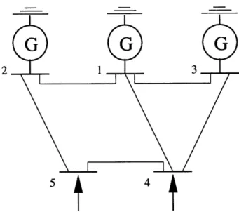
The following 5 bus network is one of the two networks that will be used in evaluating different definitions of ATC:11

2

54

₄

t

The nominal bus injections12 _{and line flows of the 5 bus network, Yinitial and}

Zinitial, are presented in Table 4.1 and Table 4.2. The final bus injections and line flows resulting from calculating STC with the linear model, Yfinal and Zfinal, as well

as the line flow constraints, Zmax, are also included as a basis for comparison.13

Table 4.1: Nominal & Final Injections for the Linear 5 Bus Network

11The network parameters are available in Appendix B

12The injection at Bus 1, the slack bus, is 0.9766 p.u. and has been held constant. 13

These nominal conditions are present before evaluating any definition of ATC.

Bus # Yinitial Yfinal

4 -1.2005 -1.8390

5 -1.1988 -2.2108

3 0.4234 0.4732

Table 4.2: Nominal & Final Line Flows for the Linear 5 Bus Network

In calculating the STC of the 5 bus network, the power received at load buses 4 and 5 was increased until a line flow constraint was violatedl4 The resulting maximum incremental bus injections are shown in Table 4.3.

Table 4.3: Incemental Injections at the STC of the Linear 5 Bus Network

Evaluating STC, which is the sum of the maximum incremental power that can be received at the load buses 4 and 5, has lead to a disproportionate increase in power injections.15 Load bus 5 receives approximately twice the incremental injection of load bus 4, and generator bus 2 almost exclusively provides this incremental injection to both loads.

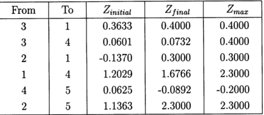
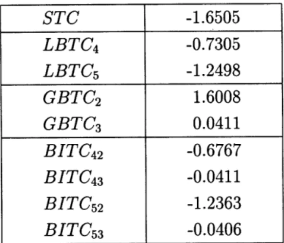
The results of evaluating the other definitions of ATC with the linear model are presented in Table 4.4. These results indicate that the available transfer capability for a power transfer across the 5 bus network strongly depends upon the associated

1 4

Table 4.2 shows that line31, line21, and line25 were the first to reach their maximum capacity.

15

Evaluating STC implies that both load buses are participating in a power transfer from both generator buses.

From To Zinitial Zfinal Zmax

3 1 0.3633 0.4000 0.4000 3 4 0.0601 0.0732 0.4000 2 1 -0.1370 0.3000 0.3000 1 4 1.2029 1.6766 2.3000 4 5 0.0625 -0.0892 -0.2000 2 5 1.1363 2.3000 2.3000 Bus # Yinc 4 -0.6385 5 -1.0120 3 0.0498 2 1.6008

Table 4.4: ATC Definitions Evaluated with Linear Model on the 5 Bus Network origin and destination buses. Consequently, the different definitions of ATC can lead to significantly different evaluations of how much power can be transferred.

For example, the value of LBTC4 suggests that load bus 4 has less than half the

capability of receiving power than would be indicated by the STC alone. Moreover, within the context of a specific bilateral power transfer from generator bus 3 to load bus 4, the STC provides no meaningful indication of how much power can actually be transfered, as can be seen from the value of BITC43.

Another important observation is the significant difference between the maximum power that can be injected by buses 2 and 3. Although generator bus 2 can use the STC as a good indication its available transfer capability, generator bus 3 has only a marginal transfer capability and cannot use the STC to make any decisions about how much power it can inject.

STC -1.6505 LBTC4 -0.7305 LBTC5 -1.2498 GBTC2 1.6008 GBTC3 0.0411 BITC42 -0.6767 BITC43 -0.0411 BITC5 2 -1.2363 BITC5 3 -0.0406

4.4

39 Bus Network

The second network used to evaluate ATC definitions is the 39 bus network repre-sented by the following schematic 6:

Load Buses m . I

I

r

.

I

I

I I

Figure 4-2: 39 Bus Network

The results of evaluating some ATC definitions on the 39 bus network with the linear model are shown in Table 4.5. The difference between STC and GBTC3 8

is considerable, which implies that generator bus 39 should be careful about making decisions about how much power to inject based solely on the information provided by the system transmission capacity.17 Moreover, there is little conformity in the amount of power that can be received by different load buses either in bilateral transfers or from the entire network.

Table 4.5: ATC Definitions Evaluated with Linear Model on the 39 Bus Network

'6The network parameters are available in Appendix B 17Note that STC is the current industry definition of ATC.

Slack Bus - 39 STC -8.0100 LBTC1 -3.0000 LBTC2o -1.3200 GBTC3 8 2.5000 BITC138 -1.5295 BITC20-38 -0.5208

Chapter 5

Non-Linear Model-Based ATC

Calculations

5.1

OPF with Coupled Load Flow Equations

The nonlinear model that is used to calculate the different ATC definitions uses coupled load flow equations without any simplifying assumptions. Using computer simulation, an optimal power flow scenario is formulated that minimizes' incremental power injections at all relevant load buses. In general, an optimal power flow solves the basic load flow problem2 according to some set of constraints while optimizing a desired performance index. The set of constraints used are the maximum line flows, and the performance index chosen is the sum of incremental injections at all participating load buses.3

1Incremental load is defined as being negative.

2_{See Appendix A for a derivation of the basic load flow problem.} 3

5.2

5 Bus Network

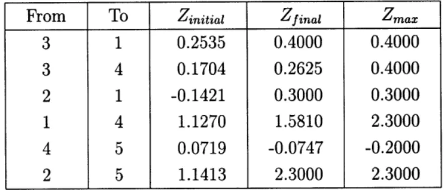
The nominal and final conditions resulting from using the nonlinear model to evaluate the STC of the 5 bus network are presented in Table 5.1 and Table 5.2.4

Bus # Yinitial Yfinal Vinitial Vfinal Oinitial Ofinal

4 -1.2005 -1.8662 0.9865 0.9789 -0.0091 -0.0107

5 -1.1988 -2.1710 0.9877 0.9776 -0.0249 0.0064

3 0.4234 0.6625 1.0000 1.0000 0.0230 0.0345

2 0.9992 2.6000 1.0000 1.0000 -0.0144 0.0303

1 1.0680 0.9995 1.0000 1.0000 0 0

Table 5.1: Nominal & Final Conditions for the Nonlinear 5 Bus Network

Table 5.2: Nominal & Final Line Flows for the Nonlinear 5 Bus Network This nominal bus injections of the nonlinear model are identical to those of the linear model except for the increased power injected at the slack bus, which is included here to show the effect of loss compensation." Moreover, the nominal line flows are comparable, though not identical, to those of the linear model. After maximizing the incremental power received at the load buses, the resulting bus injections and line

4_{The values presented in theses tables are defined analogously to the ones used in Table 4.1 and} Table 4.2. Note the additional values for bus voltage (Vinitiai, Vfinal) and phase angle (Oinitial, Ofinal)

resulting from using the nonlinear model. 5

The slack bus has been allowed to have a small but nonzero change in reaching a solution with the nonlinear model. This has been done for ease of calculation in the presence of losses and does

not affect the meaning of the results.

From To Zinitiai Zfinal Zmax

3 1 0.2535 0.4000 0.4000 3 4 0.1704 0.2625 0.4000 2 1 -0.1421 0.3000 0.3000 1 4 1.1270 1.5810 2.3000 4 5 0.0719 -0.0747 -0.2000 2 5 1.1413 2.3000 2.3000

flows are also very similar to the values obtained using the linear model. In fact, the same lines reach their flow constraints at the STC evaluated with both models.6

Table 5.3: Incemental Injections at the STC of the Nonlinear 5 Bus Network

The distribution of incremental bus injections in evaluating the STC of the 5 bus network with the nonlinear model are also comparable to the values obtained with the linear model. The only significant difference is the increased power injection at bus 3 which results because of the presence of losses when using the nonlinear model.

Table 5.4: ATC Definitions Evaluated with Nonlinear Model on the 5 Bus Network Although the differing results of evaluating each ATC definition with the linear and nonlinear models cannot be predicted with certainty, it can be seen that in most cases the linear model overstates available transfer capacity. Nevertheless, the results obtained from the nonlinear model are very similar to those obtained from the linear

6_{These lines are line}

3l, line21line25. Bus # Yinc 4 -0.6657 5 -0.9722 3 0.2391 2 1.6008 STC -1.6379 LBTC4 -0.7553 LBTC5 -1.2006 GBTC2 1.5999 GBTC3 0.1718 BITC42 -0.6050 BITC43 -0.0284 BITC52 -1.1695 BITC5 3 -0.0258

model, reinforcing the observation that different ATC definitions have an impact on the available transfer capability of a network that cannot be ignored.

5.3

39 Bus Network

It is not an easy task for the nonlinear model to converge to a solution with the 39 bus network. The load flow equations are difficult to solve in general, and when the set of constraints imposed by the optimal power flow formulation are applied, the probability of finding a feasible solution further diminishes. The following results are presented as a comparison with those of the linear model, as well as a confirmation of the validity of previous observations when using the nonlinear model on the 39 bus network.

STC -5.2971

LBTC1 -1.9968

LBTC2o -1.3185

Table 5.5: ATC Definitions Evaluated with Non-linear Model on the 39 Bus Network

Although the values for LBTC are comparable to the results of the linear model, the STC of the 39 bus network is significantly lower. Once again, the linear model has overstated the ATC of the transmission network due to the simplifying assumptions it makes. Nevertheless, the difference between STC and how much power can be received by a load bus from the entire network is apparent from the results in Table 5.5. It should be mentioned here that the computing time necessary to arrive at the results presented in Table 5.5 was approximately 30 minutes on a SGI workstation. This implies that serious computational power would be required if more extensive ATC information is demanded in real time.

Chapter 6

Changing System Parameters

6.1

Flow Constraints

It is clear that increasing the line flow constraints of a network will generally increase ATC regardless of which definition is used. Table 6.1 shows some results of evaluating the STC, LBTC, and BITC of the 5 bus network with the linear model. Uniform flow constraints are used on each transmission line for simplicity. It is interesting to note that increasing flow constraints has a more pronounced effect on STC than BITC because the incremental power can be more widely distributed throughout the network. An important implication here is that STC, as a definition of ATC, is more sensitive than other definitions to wrong estimates or growth forecasts of the line flow capacities of a transmission network.

ATC Definition Zmax = 3 Zmax = 4 Zmax = 5

STC -3.9601 -6.0799 -8.1997

LBTC4 -2.8327 -4.4090 -5.9852

BITC43 -2.1356 -3.3239 -4.5122

6.2

Dependence on the Choice of a Slack Bus

Changing the slack bus not only affects the evaluation of ATC, but also the nominal load flow conditions. The following results illustrate the effect of changing the slack bus upon nominal bus injection, Yinitial, as well as STC, LBTC, and BITC on the 5 bus network. The nonlinear model has been chosen because the linear model does not allow the slack bus to change when maximizing incremental injections. Consequently, the values obtained will not be affected by any constraints imposed on the slack bus explicitly by the calculations.

Table 6.2: The Effect of Changing the Slack Bus on Yinitial

Table 6.2 shows that changing the slack bus has a nonzero effect on the nominal injections at the buses being switched. Other bus injections cannot change because they are defined as inputs to the load flow problem.' However, without redefining the nominal power injections at the generator buses, which are typically not identical, simply switching slack buses will generally have a nonzero impact on the initial load flow solution.2

Switching the slack bus seems to have a more significant effect on STC and LBTC than on BITC. In fact, while Table 6.3 shows a dramatic change in LBTC4 and

LBTC5 due to the change of slack bus, neither BITC43 nor BITC5 3 show any change

at all. This is not the case in general, but it is a fair observation that the BITC between two particular buses is not as sensitive to changing the slack bus as other

1

See explanation of PV and PQ buses in Appendix A. 2

This is also true when using the linear model.

Bus # Slack Bus 1 Slack Bus 2

4 -1.2005 -1.2005

5 -1.1988 -1.1988

3 0.4234 0.4234

2 0.9992 0.9995

Table 6.3: Evaluating ATC definitions with Different Slack Buses

ATC definitions. The reason behind this observation is that, when evaluating STC or LBTC, one of the generators supplying the load buses is affected when the slack bus is switched. On the other hand, since the generator in a bilateral transfer cannot be the slack bus by definition, changing the slack bus should only have a marginal impact on BITC if any at all.

ATC Definition Slack Bus 1 Slack Bus 2

STC -1.6379 -1.4179

LBTC4 -0.7553 -1.3433

LBTC₅ -1.2006 -0.2363

BITC43 -0.0284 -0.0284

6.3

Voltage Constraints

The effect of imposing voltage constraints on the evaluation of ATC is exclusive to the nonlinear model.3 The relationship between voltage and transfer capability has already been explored in other studies [17]. For example, it has been shown that the difference between the voltages at the generator and load buses is directly proportional to the real power transfer capability of a network.

Therefore, it makes sense that as the minimum load bus voltage allowed on the 5 bus network increases, which effectively lessens the difference between generator and load bus voltages, all ATC values should generally decrease. Although this re-lationship is not strictly held due to the nonlinearity of the load flow equations, the following figures show that STC, LBTC, and BITC will generally decrease as volt-age constraints restrict the load bus voltvolt-ages from moving away from the generator bus voltages.

O

I-(I)

U.93 U.94 U.Ub U.Uj V.u.I u.%PO minimum load bus voltage

Figure 6-1: Variation of STC with Voltage Constraints

.Q4IT

CO

5n

Hj

0.93 0.94 0.95 0.96 0.97 0.98

minimum load bus voltage

Figure 6-2: Variation of LBTC4 with Voltage C

UO 0 co CU .0 E o O m Figure 6-3:

minimum load bus voltage

Variation of BITC42 with Voltage Constraints

The data points used in the figures above are available in Appendix D. The re-lationship between minimum load bus voltage and the various definitions of ATC appear relatively linear. Moreover, the effect of changing voltage constraints on STC seems more unpredictable than on LBTC or BITC.

Chapter 7

Conclusions

Although using a system transmission capacity to represent ATC can provide a general indication of a network's level of congestion, it has been shown that in many cases the transfer capability available to network buses needs a more accurate representation. More specifically, the results obtained from the computer simulations developed for this thesis indicate that it is meaningful and necessary to utilize definitions such as LBTC, GBTC, and BITC to characterize the capability of power transfers on a transmission network depending on the type of energy market in place.

Not only have the results obtained shown a significant difference between values of STC and other definitions, but also between the values of the ATC definitions themselves. Some relevant implications that have emerged from the results are that:

1. GBTC can be used as an indication of how advantageous one generator's po-sition on a transmission network is relative to other generators in terms of the maximum incremental power it can inject beyond some nominal operating con-dition.

2. There is an important distinction made by the difference between LBTC and BITC regarding the maximum power that can be received by a load bus through the network. For example, even though each bus has a unique LBTC at each moment in time, the power it can receive from different generator buses can vary significantly. Thus, even LBTC cannot be used too freely in determining

the ATC of a bilateral power transfer.

3. STC is more sensitive than other ATC definitions to changing system parame-ters such as line flow constraints, voltage constraints, and choice of slack bus. Thus, any errors in calculating or forecasting theses system parameters will have a more significant impact on the values of STC.

There are many remaining open questions concerning the meaningful concept of ATC. One obvious next step would be to study the implications of these definitions on computing physical limits of a large interconnection comprising several energy markets.

Appendix A

Basic Load Flow Problem

Each line in a power network connecting a pair of buses can be modeled as follows:

Bus 1 Bus 2

Figure A-1: Model of Transmission Line

where R12 and X12 and the lumped resistance and reactance of the entire line12.

The complex power S12 on the transmission line sent from bus 1 to bus 2 is defined in terms of the complex bus voltages and network parameters as

S12 - V1/ I 2 = V1 - V2* (V - V2) Y*2 -- (V2

-

V V2*) Y12

where * denotes a complex conjugate and Z12 = R12 + j X12 = Y.

The real power P12 and reactive power Q12 injected at bus 1 are obtained by

taking the real and imaginary parts of S12. Since V and V2 are complex, V -V2* may

be expressed as ]V IV2

I

S1 2 = (IVl 12 - IVlllV2 ei("-2)) - (G1 2 - jB12)

where Y12 = G12 + j B 12 and 612 = 61 - 62. Using this representation of S12, the real and reactive power injected at bus 1 may be separated and expressed in terms of real voltage magnitudes, phase angle difference, and network parameters as

P12 = (V2 - V1V2 cos 612) G12 - B12 V1V2 sin 612

Q12 = -(V 2 - VV2 COS 612) B 2 - G12 VV2sin12

In formulating the basic load flow problem, all the load buses of a network are specified as PQ buses where real and reactive power are given. Similarly, all generator buses except one, the slack bus, are specified as PV buses where the real power and bus voltages are given. The slack bus is a generator bus which is specified as an ideal voltage source with Vla,,k = 1 ej-0

The basic load flow problem is the solution of all bus voltages Vi, phase angles

6i, and real and reactive power injections Pi and Qi at each bus i, given the network parameters and specifications of the PQ and PV buses. This problem must be solved iteratively with numerical techniques such as the Newton-Raphson method'.

In order to solve the load flow problem [18], the equations specifying the real and reactive power through each line must be used in conjunction with Kirchoff's law at each bus (Pi = Ejec Pij and Qi = Ejcc Qij where Ci indicates all lines connected to bus i). The set of these equations for bus injections and line flows are the coupled load flow equations. The role of the slack bus in solving these equations is compensating for transmission losses.

It is often more convenient to use a per unit system [18] when calculating power flows. This is done by expressing all electrical quantities as proportions of appropri-ately chosen reference levels. For example, if these reference levels are specified as

Vref = 50 kV and Irf = 1000A, then the electrical quantities of a bus operating at 52 kV and injecting 1100 A can be normalized to V = 52 _{50 -} 1.04 p.u., I = 1100 ₁₀₀₀ = 1.1 p.u.. Other quantities such as power and impedance can be similarly normalized.

1_{A description of the numerical techniques used to solve the load flow problem is beyond the}

Appendix B

Network Parameters for the 5 and

39 Bus Networks

Table B.1: 5 Bus Network Parameters

The line flow constraints, Zmax, were chosen after analyzing the nominal line flows of the 5 bus network using both the linear and nonlinear models. This was done to insure that a feasible solution existed prior to any maximization of incremental power injections.

To 1 1 1 2 2 3 3 4 4 5 5 6 6 7 8 9 10 10 13 14 15 16 16 16 16 17 17 21 22 23 25 26 26 26 28 2 6 6 10 12 12 19 19 20 22 23 25 29 R From

X

Table B.2: 39 Bus Network Parameters

Zmaz R X 0.003500 0.002000 0.002000 0.001300 0.007000 0.001300 0.001100 0.000800 0.000800 0.000200 0.000800 0.000600 0.000700 0.000400 0.002300 0.001000 0.000400 0.000400 0.000900 0.001800 0.000900 0.000700 0.001600 0.000800 0.000300 0.000700 0.001300 0.000800 0.000600 0.002200 0.003200 0.001400 0.004300 0.005700 0.001400 0.000000 0.000000 0.000000 0.000000 0.001600 0.001600 0.000700 0.000700 0.000900 0.000000 0.000500 0.000600 0.000800 0.004110 0.005000 0.005000 0.001510 0.008600 0.021300 0.013300 0.012800 0.012900 0.002600 0.011200 0.009200 0.008200 0.004600 0.036300 0.025000 0.004300 0.004300 0.010100 0.021700 0.009400 0.008900 0.019500 0.013500 0.005900 0.008200 0.017300 0.014000 0.009600 0.035000 0.032300 0.014700 0.047400 0.062500 0.015100 0.018100 0.050000 0.050000 0.020000 0.043500 0.043500 0.013800 0.014200 0.018000 0.014300 0.002720 0.002320 0.015600

Appendix C

Optimal Power Flow Formulation

The general formulation of the OPF problem uses the same preliminary data as the basic load flow problem (network parameters and specifications of PQ and PV buses), and solves for the same variables (V, 6, P, and Q at all buses). However, there are two major departures [19].

The first one is the presence of a criterion for solving the load flow problem. This criterion is expressed in terms of the maximization (or minimization) of a performance index. In calculating ATC, this index has been defined as the sum of incremental in-jections at all load buses relevant to the definition of ATC being evaluated. The second departure is the explicit inclusion of inequality constraints that typically rep-resent the security conditions that have to be met. The only constraints that have been used in calculating ATC in this thesis, unless otherwise stated, are the flow constraints for each network.

The OPF formulation used to calculate ATC may be summarized as minimizing index =

Z

i ELA

where yi is the incremental power at bus i and La are the incremental load buses. This minimization is done subject to the equality and inequality constraints

f(vG,p, L) = 0

where f is a vector of the load flow equations (VG : generator bus voltages, p : real power at all buses, qL : reactive power at load buses) and g is a vector of the flow constraints (zij : real power flows, zim"ax : maximum real power flows).

Appendix D

Voltage Constraints and ATC

Table D.1: Data Points for Comparing Voltage Constraints with ATC Definitions The empty cells in the table above correspond to missing data points resulting from the inability of the optimal load flow simulation used to find a solution for certain combinations of voltage constraints and ATC definitions. V,min refers to the minimum load bus voltage constraint, while V4 and V are the actual voltages at buses 4 and 5

after evaluating each definition of ATC.

Vmin STC LBTC4 BITC42 V4 V5 0 -3.4410 -5.7451 0.9469 0.9824 .9250 -3.4409 -5.7140 .9350 -3.4408 -4.6655 0.9469 0.9824 .9450 -3.4408 -4.3617 -4.3617 0.9469 0.9824 .9475 -3.4063 -3.2251 0.9475 0.9822 .9500 -3.2561 -3.2271 -3.9024 0.9500 0.9817 .9550 -2.9380 -2.9790 -3.4251 0.9550 0.9805 .9650 -2.6157 -1.9651 -2.2820 0.9669 0.9650 .9700 -2.6761 -1.7920 -1.8731 0.9700 0.9700 .9750 -0.9774 -1.2659 -1.3356 0.9785 0.9864 .9800 -1.3409 -0.6924 -0.4123 0.9802 0.9800 .9825 -0.8518 -0.4150 0.9825 0.9832 .9850 -0.4090 -0.1791 -0.1793 0.9850 0.9850

Bibliography

[1] Federal Energy Regulation Commission. Order No. 888, April 1996.

[2] North American Electric Reliability Council. Available transfer capability defi-nitions and determination. Technical report, NERC, 1995.

[3] North American Electric Reliability Council. Glossary of terms. Technical report, NERC, August 1996.

[4] National Science Foundation. Proceedings of the Workshop on Available Transfer Capability, June 1997.

[5] M. Ilic and F. Galiana. Power Systems Restructuring; Engineering and Eco-nomics, chapter 2. Kluwer Publishers, 1998.

[6] M. Ilic, F. Galiana, L. Fink, A. Bose, P. Mallet, and H. Othman. Transmission capacity in power networks. International Journal of Electrical Power and Energy System, 1998.

[7] Assef Abdulla Zobian. A framework for pricing transmission and ancillary ser-vices in competitive electric power markets. Master's thesis, MIT, 1995.

[8] Joaquin Ramon Lacalle Melero. Short term analysis of electrical energy markets under reat time pricing. Master's thesis, MIT, 1993.

[9] Pedro Alfonso Lerner. On the value of transmission systems under open access : incentives for investment. Master's thesis, MIT, 1997.

[10] Edo Macan. Peak-load transmission pricing for the ieee reliability test system. Master's thesis, MIT, 1997.

[11] Felix Wu, Pravin Varaiya, Pablo Spiller, and Shmuel Oren. Folk theorems on transmission access:proofs and counterexamples. The Electricity Journal, Octo-ber 1994.

[12] Marija Ilic, Eric Allen, and Ziad Younes. Providing for transmission in times of scarcity: An iso cannot do it all. May 1997.

[13] Felix F. Wu and Pravin Varaiya. Coordinated multilateral trades for electric power networks: Theory and implementation. Technical report, University of

California Energy Institute, June 1995.

[14] M. Ilic and J. Zaborszky. Dynamics and Control of the Large Electric Power Systems. Wiley Interscience, 1998.

[15] M. Ilic and F. Galiana. Power Systems Restructuring; Engineering and Eco-nomics, chapter 3. Kluwer Publishers, 1998.

[16] F.C. Schweppe, M.C. Caramanis, R.D. Tabors, and R.E. Bohn. Spot Pricing of Electricity. Kluwer Academic Publishers, 1988.

[17] Santiago Banales and Marija D. Ilic. On the role and value of voltafe support in a deregulated power industry. North American Power Symposium, October 1997.

[18] Electric Power Research Institute. A Primer on Electric Power Flow for Economists and Utility Planners. Incentives Research Inc., 1995.

[19] O.I. Glgerd. Electric Energy Systems Theory: An Introduction. McGraw-Hill Inc., 1971.