AN ARITHMETICAL MODEL OF SPATIAL DEFINITION by Duncan S Kincaid
BSc, BA, Tulane University New Orleans, Louisiana May 1984
Submitted to the Department of Architecture on June 6, 1997 in partial fulfillment of the requirements for the Degree of Master of Architecture at the Massachusetts Institute of Technology
September 1997
@ Duncan Kincaid 1997. All rights reserved
The author hereby grants MIT permission to reproduce and distribute publicly paper and electronic copies of this thesis document in whole or in part.
Signature of Author .... . ... . ... dskincaid
Certified by ... Maurice K Smith
Professor of Architecture, Emeritus
Thesis Supervi
Accepted by.. Wellington Reiter
Chairman, Committee on Graduate Students
A."
897
Aaron Fleisher
Senior Lecturer of Architecture, Emeritus
Fernando Domeyko
Senior Lecturer of Architecture
AN ARITHMETICAL MODEL OF SPATIAL DEFINITION by Duncan S Kincaid
Submitted to the Department of Architecture on June 6, 1997 in partial fulfillment of the requirements for the Degree of Master of Architecture
Abstract
The manner in which spatial definition is built by architectural form is identified and
forma-lised in part. A description is given for the structure of spatial definition. This description allows for a mapping from the class of uses to the class of spatial structures.
Thesis Supervisor: Maurice K Smith Title: Professor of Architecture, Emeritus
I don't know that the aforementioned would appreciate these ideas or their execution. The simplicity of the abstraction and errors in my understanding of form is sure to disappoint any designer and thinker of their caliber. But what we've in common I think more deep than the differences are numerous. And that is the position that architecture is an empirical art and science, one which admits to empirical facts and belongs as much to the human intel-lect as spirit
if there a difference.
Acknowledgment
and
TABLE OF CONTENTS
Introduction
1.1 A b stract ... 9 1.2 Related work.. ... 11
1.2.1 Past formalisations of spatial definition 11 1.2.2 Formalisations of spatial definition in knowledge-based systems 13 1.3 Disclaimer 15 Spatial Model 2.1 T erritory ... 17 2.1.1 Registration model 18 2.1.2 Field model 20
2.1.3 Equivalency of the two models 21 2.1.4 General observations 22
2.2. Applicability of spatial model to all spatial extents 2.2.1 Planar spatial extents 23
2.2.2 Curved spatial extents 25 2.2.3 All spatial extents 26
Arithmetic Model
3.1 A ddition on territory... 27 3.1.1 Determination of D 28
3.1.2 Determination of $a e p 30
3.2 Additional field structure ... ... 33 3.2.1 Degree of definition 33
3.2.2 Field bias 33
3.3 C on trol... 35 3.4 Union of territories ... 36 3.5 Exam ples ... 37
3.5.1 Example la: Curved extents: intrinsic control 37 3.5.2 Example 1b: Curved extents: extrinsic control 38 3.5.3 Example 2: Rectilinear extents 40
Use Model
4.1 Access/Go definitions... 44 4.1.1 Necessary and sufficient conditions for access/go
field 44
4.1.2 General conditions 44
4.2 Privacy/Stop definitions ... 46 4.2.1 Necessary and sufficient conditions for privacy/
stop field 46
4.2.2 General conditions 46
4.3 Collective/Slack definitions... 48 4.3.1 Necessary and sufficient conditions for collective/
slack field 48 4.3.2 General Conditions 48 4.4 C ase Studies... 50 4.4.1 Access/Go 50 4.4.2 Privacy/Stop 54 4.4.3 Collective/Slack 58 4.5 Size ... 62 Concluding Remarks 5.1 Other applications ... 63 5.2 Concluding remarks... 65 Appendices Appendix A: Ensembles ... 67 Appendix B: Classes and Methods... 75
References
R.1 Bibliography... 77 R.2 Illustration credits ... 80
CHAPTER 1
|N
T R O D U C T 1 O N.what did you do after you'd made certain that you'd done nothing at all?...
-Sherlock Holmes to Inspector Hop-kins after the latter's investigation in The Case of the Golden Pince-Nez (as told by M K Smith to dskincaid apropos...)
1.1 Abstract
Architecture practices its art and craft in the articulation of space. Building elements are necessary components of its efforts. These ele-ments may be columns, beams, walls, screens, light and assemblies of the same. Their physical attributes include dimension, colour, mate-rial, use, and tectonics.
Certain of these attributes admit to formalisation. Indeed, computer based formalisations of some already exist: CAD encodes geometric descriptions, raytracing/texture mapping encodes the interaction of light with geometry/material, structural analysis software encodes the performance of loaded members.
What remains lacking, however, is a formalisation of the architectural
behaviour of these properties. By architectural we mean spatial or terri-torial. How might structure, material, light and dimension contribute
1.1 ABSTRACT
severally and in combination to the definition of territories? What structure is exhibited by the territories so defined? Might there exist a mapping from the class of uses to these spatial structures?
This research programme should be of some interest for two reasons. The first is epistemological. The resulting formalisation may be thought as a set of axioms from which theorems describing territory are derived. As such, the calculus embodies a theory of architectural form which is testable in the built environment-scientific method is given its due in architectural discourse. This programme should also be of interest to those engaged in knowledge-based architectural design systems-for one cannot reason intelligently about architec-tural form if ignorant of the spatial commitments which lie in that form.
Towards these ends, this work begins to identify and formalise the manner in which physical and organisational properties of
architec-tural elements build territory. It also describes some properties of the territories themselves.
1.2 RELATED WORK
1.2 Related work
1.2.1 Past formalisations of spatial definition
Architecture has not been without its treatises. Vitruvius, Vasari, Pal-ladio, the Spanish Crown, the Ecole de Beaux Arts, Durand, and countless others have offered their theories of architectural form. Most all these, however, have written prescriptive rules for parti gen-eration which amount to rules of composition.
This is most unfortunate. If considered more closely, these works reveal shortcomings such as to compromise their worth. For the most part, attention is restricted to the shape of form and shape of its arrangement.1 Shape in itself is arguably the least interesting prop-erty of architectural form. It is uninteresting as it is a propprop-erty shared with every other object in the physical world. Further, an architect doesn't design with shapes but with materials and their structural properties, with light, access, spatial definition, tectonic expression,
and uses.
The prescriptive rules of these treatises are also lacking in architec-tural substance. One would expect these to address the material and formal behaviours of the architectural entities upon which they oper-ate. Rather than define rules to flag redundancies in spatial
defini-1. The Leyes de Indias of 1635 may be an exception to this, as consider-able attention was given to use organisation (Kincaid 1997).
1.2 RELATED WORK
tions, suggest access given a set of architectural conditions (such as light, public/private zones and section, among others), the rules may simply mirror or rotate a shape.
What architectural knowledge is captured by these formalisations? That bilateral symmetry rules the day, that voids are always built from a module of thus and such ratio, that perforations are axially placed? Again, these address the geometry, not architecture of the piece. They could be describing a tablecloth pattern, a waffle iron or sheet of stamps.
Of course there is much written on the subject of architectural form and space which resists formalisation.2 A number of these works are in the manner of Ramussen (1964) and Arnheim (1977) who write of architecture's experiential qualities. These at least acknowledge space and use and credit physical form as their partial determinant. Norb-erg-Schulz (1986) has concerned himself with phenomenological
aspects of architectural form, at times relegating physical space for a speculative 'existential space.'
Other works have concentrated on the sociological nature of space as in Hall (1966) and Newman (1973). Herzberger (1993), Alexander (1977) and recent thesis work at MIT address territory explicitly. Herzberger and Alexander promote an architecture of association predicated upon coherent use territory. Chong (1992) identifies
terri-2. As there is which resists comprehension, to wit Heidegger.
1.2 RELATED WORK
tories in Schindler's work, but like Herzberger and Alexander, fails explicitly to identify the means by which these are built. Reifenstein (1992) investigates 'positioning rules' which build territory and spa-tial structure. These rules beg the question, however, as they operate on territories whose definition remains unanswered. None of the aforementioned speak directly as to how physical form builds spatial definitions, nor do they formalise their findings.
1.2.2 Formalisations of spatial definition in knowledge-based systems
Computer-based systems for evaluating aspects of architectural form are many. One may partition the class into those which do not evalu-ate design with respect to geometric representations of physical form and those which do. The former would include systems reasoning on topological models for adjacency, say, or even systems representing experiential qualities but not relating them to physical form (Mortola 1991).The latter would include systems such as (Carrara 1994) and (Dave 1994) wherein design characteristics are dynamically calcu-lated on the basis of physical form representation.
Those knowledge-based systems which acknowledge physical form would surely appear better equipped. As discussed in (Koile 1997) a physical form model would facilitate computation of circulation paths, enable the computation of visual barriers (Hanson 1994) and allow for designer interaction in a mode with which he is already familiar (Gross 1996). They would be better equipped for an even more fundamental reason, however; a physical form model allows, at
1.2 RELATED WORK
least in principle, for a spatial definition model. As architects reason with spatial definitions-their dimensions, qualia, degree of
defini-tion, organisadefini-tion, and supported uses-so too should a computa-tion-based system purporting design intelligence.
Evaluative reasoning on experiential qualities such as private or open, and use ascriptions such as bedroom or entrance, say, can only fully be made in the presence of territories which support them. Likewise, ascriptions made of territories-such as dimension or degree of pri-vacy-can best be made in the presence of the physical form which builds them.
Most evaluative systems have either ignored or misused a physical form component. None have made use of a territory model. This is likely a result of not knowing how physical form builds spatial form. This work may aid in correcting the deficiency.3
3. Kimberle Koile of the MIT Artificial Intelligence Laboratory, with assistance of this author, is implementing some of these ideas (Koile 1997). Physical form is paramount in this work. From it is built a terri-tory model which in turn supports a use-space model and connectiv-ity model. A considerable, if not essential, part of evaluative
reasoning takes place at the level of territory. The territory model is constantly updated as changes are made by the user to the physical form model.
1.3 DISCLAIMER
1.3 Disclaimer
The work contained herein might best be considered an hypothesis. As with most hypotheses, it is likely wrong and certainly incomplete. There is no excuse for the former. As for the latter, it may well be the case that architecture's infinitudes will always outnumber any for-malisation's.
This model of spatial definition makes a number of simplifying assumptions and abstractions, to be sure, though none are thought to compromise the enquiry. The greatest of these is the primacy given to form's spatial extents.4 Though other attributes of form such as mate-rial and tectonics participate in the definition of territory, it is thought that they do so in a manner subsumed by spatial extents. Specifically, these secondary properties are believed to build ensembles of form which in turn induce territory as a function of the ensembles' extents. There is considerable evidence to suggest this reasonable as seen in later chapters.
For some time now the subjective and whimsical have found many champions in architectural education and practice. Though one can-not condemn a priori the subjective and whimsical, one can condemn the ignorance with which it is often practiced. This ignorance is not of
4. Spatial extents are not to be confused with material extents. A struc-tural bay, for instance, will exhibit the spatial extents of a box. These extents are composed of planes, not surfaces. Only in the trivial case of a single entity such as a column are the spatial extents coincident with the material extents and the faces rendered as surfaces.
1.3 DISCLAIMER
the latest French literary theory, German Phenomenologie, or the latest Wonder of the World Wide Web, but an ignorance of the spatial and organisational commitments which lie in architectural form. It is hoped this work may reinforce the position that architecture operates in the objective, physical world and not in that of invented discourse nor that of cyberspacial fancy.
CHAPTER 2
SP ATIAL MOD EL
The spatial extents of physicalform induce terri-tory, a model of which is given.
Spatial definition or territory is built principally through the spatial
extents of physical form. This does not discount the many other prop-erties of form which contribute to spatial definition such as material and tectonic character. As shall be argued elsewhere, these properties perform in a manner encompassed by spatial extents.
2.1 Territory
Spatial definition is recognised as an alteration in the isotropy of Space ((). Alterations appear as organisational or structural perturba-tions.
Two such structures are considered below. The first describes a spa-tial structure induced by registration from aform's spatial extents. The
second describes a directionalfield structure induced by spatial extents. In both, territory or spatial definition is specified through organisation, much as a mathematical space may be specified by a metric.
Both models are experientially based, which is to say the organisa-tions described are readable in one's experience of architectural form. Further empirical work might well suggest adjustments in the mod-els' particularities.
2.1 TERRITORY
2.1.1 Registration model
Consider the spatial extents a of some physical demarcation A. Asso-ciated with a is a measure of registration described in plan in
Figure 2.1.
(0,0 ,z)
(0 y 0O)
(0,0,0)
X
Figure 2-1
The intensity of registration from a diminishes with distance from a. It diminishes even more rapidly outside the projection of a, shown by dotted lines. As this behaviour holds uniformly for every face of a, the following discussion focuses on a single face.
2.1 TERRITORY
Intensity of registration can be described as a step function:
Ir| % 3 9 1
Ir(X, Y, Z) = 0 & x & h, -h! x 0 ir/2 h<x<2h,-2h!x<-h
=ir/4 2h<x 3h,-3h! x <-2h = 0 (3h <x<-3h
y,<y or y<O z,<z or z<O for some constant ir
Registration Ir halves with every displacement h from a. For dis-tances greater than 3h, Ir is small as to be discounted. Which is to say
the registration, hence territorial definition, vanishes to zero outside the projection of a. This does not accord exactly with facts, but should prove serviceable.
What is important in this description is that the y and z values can zero the function, but do not otherwise figure in the value of
Ir(X, y, z). Indeed, non-zero territorial definition is controlled by h,
the extent's height. It follows that a plan representation of architec-tural form does not adequately reveal territory.
As desired, territories are identified with non-zero values for Ir . They may be understood as a disruption in the isotropy of (, where I is everywhere 0. Territory is bounded by the projection of the form's spatial extents and diminishes with distance from the same.
2.1 TERRITORY
2.1.2 Field model
Spatial extents as those considered above may be said to induce another type of rent in isotropic (. The width and height of a intro-duce directional biases in ( as shown for a single face in Figure 2-2.
vertical
(j) horizontal
,t~.
44
Figure 2-2
Both directional fields $ and $aho,,zon,,, weaken as they extend beyond the width and height of the extents, as they do with increas-ing distance from the extents. Only one field is realised in experi-ence-the field coincident with direction of movement. As a result, all treatment of territory assumes a single, well-defined direction.
AN ARITHMETICAL MODEL OF SPATIAL DEFINITION
2.1 TERRITORY
This field behaviour can be described at every point by a direction given by the orientation of the inducing extent and an intensity If given by the step function below:
if 91- 91 If(x,y,z) = i; O5x5h, -h!x0 = if/2 h< x 2h,-2h < x < -h = i;/ 4 2h < x 5 3h, -3h! x <-2h = i18 3h< x< 4h, -4h! x<--3h = 0 (4h<x<-4h 2y,<y or y<-yi 2z, < z or z<-z1 for some constant if
It is significant again to note that If is largely controlled by h; side effects at the projection's extents are small, hence ignored.
2.1.3 Equivalency of the two models
Claim: The registration model given in 2.1.1 and field model given in
2.1.2 are scalar-wise equivalent.
Argument: It need be shown that Ir and If are in effect equivalent.
With domains restricted to I 13 Ir(X, y, z) w 0,
If(x, y, z) = k - Ir(x, y, z) = k - ir k = constant
if = kir
Equivalency correlates a field's intensity with the intensity of regis-tration. Field intensity, however, runs parallel with the face which
2.1 TERRITORY
induces it whilst registration intensity is normal to the same face. This is an important observation and may stated as a theorem: registration
is always normal to the associated field(s) and is of like scalar value.
In what follows, preference is given to the field definition model as it subsumes the registration model, i.e. field values bear direction as well as degree of intensity. Spatial definition, or territory, induced by extents a may then be given by
I'x = (A, $a(A))
where A denotes the set of points within the projection of ax and
(a,(A) denotes the field intensity at these points.
2.1.4 General observations
Several important observations can be made of the spatial model described above. These observations are treated in greater depth in ensuing sections.
e It is evident that spatial extents' faces induce territory. These faces are described geometrically as planes. This greatly facili-tates the model's application to spatial extents more complex than those considered thus far. This is done in Section 2.2 below.
e The territory associated with physical form A is described wholly in terms of A's spatial extents a. Outside of these spatial extents,
2.2 APPLICABILITY OF SPATIAL MODEL TO ALL SPATIAL EXTENTS
no more is said of A. The implications are great. For one, the model applies to the full range of physical form, independent of size, material, orientation and complexity. For instance the spatial extents described by the extruded parallelogram in Figure 2-2 might well accommodate a structural bay, a piece of section, a
screen or a simple wall.
e The model also allows for physical form to operate territorially at different sizes and as a part of different extents concurrently. For example, the columns which build a structural bay claim territory at the size of their own extents (material size), whilst also contrib-uting to the spatial extents of the bay (which claims territory at the size of its extents, i.e. room size).1
2.2 Applicability of spatial model to all spatial extents
It is argued below that the territory model accommodates all spatial extents as it accommodates all planar and curved extents.
2.2.1 Planar spatial extents
Claim: All planar spatial extents may be described by a finite number
of planes.
1. An ensemble is formed by shared control of its constituents' territory. Control is discussed in Chapter 3. Ensembles are treated in detail in Appendix A.
2.2 APPLICABILITY OF SPATIAL MODEL TO ALL SPATIAL EXTENTS
Argument: Planar spatial extents, by definition, are comprised of a
finite number of planar faces (i.e. planes).
/
4-/
'4
AN4 ARITf*&T1CAL MOEL OF SpATnA1 DEFOSTION
Figure 2-3a/2-3b
Figures 2-3a and 2-3b illustrate the spatial extents and induced terri-tories given by 3 and 5 planar faces respectively. Note that territerri-tories overlap within the extents. An addition defined on territory in Chap-ter 3 shows these to be zones of field intensification. Considered as footprints of buildings, one can readily see why entries should not be placed at corners; there is no territorial demarcation at corners.
2.2 APPLICABILITY OF SPATIAL MODEL TO ALL SPATIAL EXTENTS
2.2.2 Curved spatial extents
Claim: Curved spatial extents can be described adequately as a sum of
planes.
Argument: Curved spatial extents of any degree can be described
ade-quately as a sum of arbitrarily small tangent planes given by the set of tangent vectors at any point.
1AA
Figure 2-4a/2-4b/2-4c
Consider a simple curvilinear form (Figure 2-4a) with the gross pla-nar approximation of Figure 2-4b. Treating plapla-nar segments severally, the territory map is that of Figure 2-4c.
2.2 APPLICABILITY OF SPATIAL MODEL TO ALL SPATIAL EXTENTS
As the planar approximation improves, there is a propensity for the arc shaped territory to complete itself as a circle. Of course the degree to which this phenomenon occurs depends on the ratio of height and diameter of the inducing extents.
The field description of curved territory is a little more complex. Assuming uniformity in height for the concave extent (which has been the case throughout), field lines stitch themselves into concen-tric arcs. Some ratios of height to diameter allow the arcs to complete as circles with varying If. The portion of the circle in closest proxim-ity to the extent bears a greater If than that portion furthest from the extent. This is in accord with experience; spatial definition is palpably greater within the bounds of the curvilinear form than without.
With assistance from field arithmetic, Section 3.5.2 demonstrates why convex extents refuse to build a unified and inclusive territorial defi-nition, whilst concave extents do.
2.2.3 All spatial extents
Claim: Territory is a necessary consequence of physical form. Argument: All form bears spatial extents which at the minimum may
be identified with its material extents. Spatial extents generate terri-tory. Therefore, territory is always induced by physical form.
CHAPTER 3
ARITH M ETIC MODEL
An arithmetic is defined for both orthogonal and non-orthogonal overlap-ping territories.
A spatial model has been sketched in Chapter 2 in which minimally convex form elicits overlapping territories-as does compound assemblies of form of which architecture is usually comprised.
There is no a priori reason for overlapping territories to be of any spe-cial interest or consequence. However experience suggests otherwise as does the spatial model in which every (x, y, z) in an overlap bears an i value from more than one inducer.
3.1 Addition on territory
Definition: Addition on territory
Let F. and FP denote the territories built by demarcations A, B with spatial extents c and $ respectively. As per Chapter 2, these territories are described by
ra
- (A, $a(A)) Fp (B, $p(B))where A and B denote the set of points in the projection of ca and
,
and 0$a(A) and $p(B) denote directional field definition at points in A and B.Let ( denote the set of all territories.
3.1 ADDITION ON TERRITORY
The addition of IF, and F0 denoted by the symbol rV e p is defined as a mapping
(D | 1-a, rs = Fa e p = ((A G B), $ p(A G) B))
This arithmetic maps two territories to a third such that the third is comprised of points A ® B and directional field definition
p(A B). The function ® is described in section 3.1.1 whilst $ is described in Section 3.1.2.
3.1.1 Determinationof D
Definition: Addition of A and B
Let
H
denote the set of all subsets of 93 A denote the set of points inF(
B denote the set of points in
rp
The addition of A and B, denoted by the symbol A B B is defined as a mapping
® |IH, H->H @ A,B = (AnB)
3.1 ADDITION ON TERRITORY 3.1.1.1 Properties of @ : for VA, B, C E f: 1. closure A, B e
H, 3(A
@ B) = (A r B) E H 2. commutativeA@B = (AnB) = (BnA) = B@A
3. associative (A@B)@C = (A@B)n 4. unit ADH =1GA = A 5. zero ((A rB)nC) (A n (B n C)) (An(BDC)) (A @(B (@ C)) A@0=0EDA=0 6. no inverse -,3 A AA = A- IA =
n
If there were an inverse defined for D then ( @ , H) would have formed an abelian group. As it stands, ( ,
H)
forms an abelian semi-group.3.1 ADDITION ON TERRITORY
3.1.2 Determination of $a @ p
Every element in $a can be treated as a vector with a direction that of its inducer a and with magnitude If as described by the step func-tion in Secfunc-tion 2.1.2. Adding direcfunc-tional fields $a, $s -as required by the definition of
ra
e p -should then amount to vector addition on the shared elements of 0a and $p.Definition: Let d be a vector in $a. The norm or length of d is denoted
by ||d|| and is valued at If,.
Definition: Addition of $a and $p
Let
$a denote the field associated with F, $p denote the field associated with
Eg
d and3
be vectors in $a and $p respectivelyfor some shared (x, y, z)
0 denote the angle d makes with
3
The addition of $ and Op denoted by the symbol a e is defined as a mapping
E| = $a E p
= vector of norm I
and relative direction 9
3.1 ADDITION ON TERRITORY
where
f Ildt + 01= (l|dII2 + 1|2+2d )12
=
(|a||2
+||I1|2 +2|
|d
1$
cos
1/2and
9 = asin
lall
sin
0Figure 3.1 shows examples of territory addition. Note that Ia e p is defined for that region formed by the intersection of A's and B's pro-jected extents. (In the interests of clarity, only that territory associated
with the largest extents is drawn.)
r
S5
p
Figure 3-1
AN ARITHMETICAL MODEL OF SPATIAL DEFINITION
3.1 ADDITION ON TERRITORY 3.1.2.1 Properties of a e P for Va, p, yP E : 1. closure 2. commutative 0 =)=ep 3. associative $<(csey = p+ =( +) = d+cx($pey)$a (p & y) 4. unit
$a ( = D $ where 0 is the 0-vector 5. no inverse
as 0a
P is always normalised to 0
<9,
P < 7 ( , $) forms an abelian semi-group.3.2 ADDITIONAL FIELD STRUCTURE
3.2 Additional field structure
Analysis of ae p reveals additional information as to the field
struc-ture of Fa p
-3.2.1 Degree of definition
Definition: The degree of definition for any territory is the number of
overlapping territories which build it. Degrees of definition add as one would expect, i.e.
degree-defa e p = degree-defa + degree-defg.
3.2.2 Field bias
Definition: Afield bias for any territory 1a @ p is that field associated
with (max ||d||
d|ll
). Intuitively, a field bias is evident when fields are disproportionately strong, thereby favouring association with one inducer over another.Definition: Afield bias value for any territory 'a e is given by ||1d| -
||$1|.
This value is an abstraction with no real world counter-part. It gives some indication as to the strength of the field bias.3.2 ADDITIONAL FIELD STRUCTURE
Definition: When two fields add, each makes a contribution to the
other's If .Field gain describes this amount and is given by $a-gain
and $p-gain below.
$a-gain projection of
$
along d_ ||
ll1cos
9 _dilcose
$p-gain projection of df along
$
_ ||d|cos 9
Definition: Let 9 be the angle between d and
1
ande
be the angle (d + 0) makes with d. $p is said to interfere with Oareduc-0
tively when 0 > . Otherwise $p interferes constructively (d +0), d 2
with Oa .Similarly for $a interfering with $pg.
Though $,-gain and $p-gain are always positive by definition, the net contribution of components can favour one inducer over another. This leads to the constructive and reductive interference signalled by
0 above.
3.3 CONTROL
3.3 Control
Planar and curvilinear extents were shown to be reducible to a sum of planes in Chapter 2. There remains, all the same, a fundamental dif-ference in their respective territory. This difdif-ference lies in the manner in which the territory is controlled.
Definition: A territory Ia e
p is said to be controlled where If is an
absolute maximum in the regionFa
u IF .Planar extents control their territory with their inducing faces, whilst curvilinear extents often have territory controlled outside the extents, as seen in Example lb of Section 3.5.2.
For gentle curvature with respect to height, the curvilinear form behaves much as do simple planar extents; the face of the curvilinear form controls the territory with geometry outside the extents. This may be seen in Example la of Section 3.5.1.
Definition: Territory which is controlled by inducing extents is said to be intrinsic.
Definition: Territory which is controlled by geometry outside the
extents is said to be extrinsic.
3.4 UNION OF TERRITORIES
Claim: Intrinsic and extrinsic properties partition the class of
territo-ries.
Argument: Every territory bears a maximum If value somewhere.
This value obtains either at the inducer's extents (intrinsic) or else-where (extrinsic).
3.4 Union of territories
Sections 3.1.1 and 3.1.2 showed that intersecting territories build additional territories. A union of territories does not produce any additional field intensification, hence does not build any additional territory. This is confirmed by the arithmetic defined on $.
3.5 EXAMPLES
3.5 Examples
3.5.1 Example la: Curved spatial extents: intrinsic control
3V5',
kV.if
'If
0'
Figure 3-2
h = 4' , 0 = 200 between each approximating element a, P, y
1. Approximating territories a', IF,
ry
fail to overlap owing to a height of only 4 feet for the element.2. Territorial control remains intrinsic, and the curved extents behave much as a simple planar extent.
3.5 EXAMPLES
3.5.2 Example 1b: Curved spatial extents: extrinsic control
Aa
14--Figure 3-3
h = 10', 0 = 200 between each approximating element a, $, y
1. Approximating territories F,, Fo, FY overlap owing to a height of 10 feet.
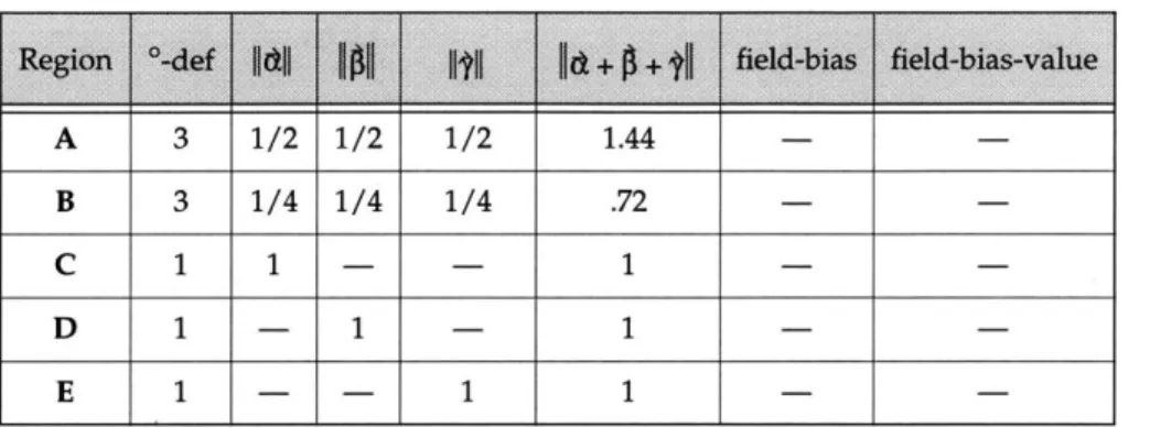
2. Maximal If in region A, hence control is extrinsic. Values are documented in Table 3-1.
AN ARITHMETICAL MODEL OF SPATIAL DEFINITION V
B 3 1/4 1/4 1/4 .72 -
-C 1 1 - - 1
D 1 - 1 - 1
E 1 - - 1 1 -
-Table 3-1: Calculated values for Figure 3-3
Notes:
1. Region A displays the greatest degree of definition and i value. As a
result, it is said to control that territory generated by the concave face. As region A lies outside the extents of the curvilinear form, the control is said to be extrinsic.
2. As the planar approximation to the curvilinear form improves, region A approaches a line in 3-space.
3. Regions C, D, E do not intersect (as told by degree-def = 1). There is no
possibility for field intensification with convex form. Control is strictly intrinsic.
3.5 EXAMPLES
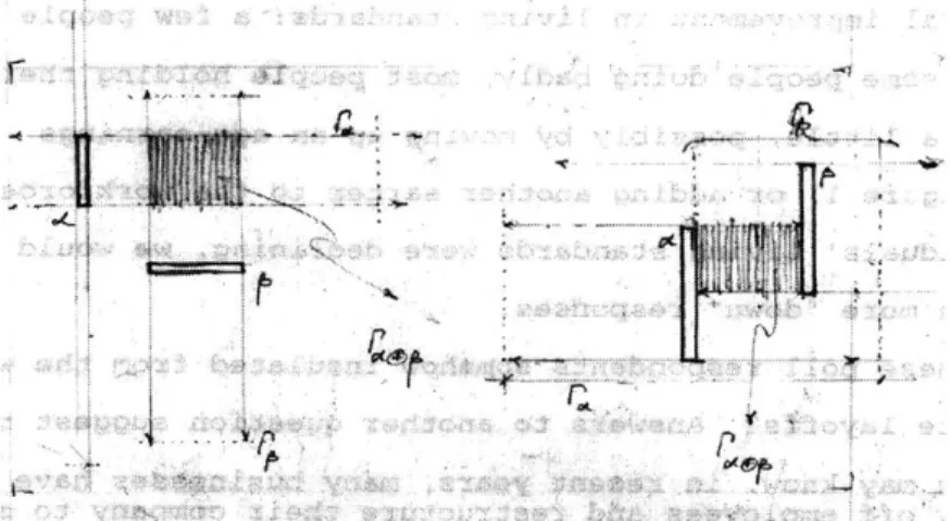
3.5.3 Example 2: Rectilinear extents
P
/
I
Figure 3-4
0 = 60',ha = 16', hp = 8'
1. Ie P is represented by the shaded region.
2. If values vary within
F, e
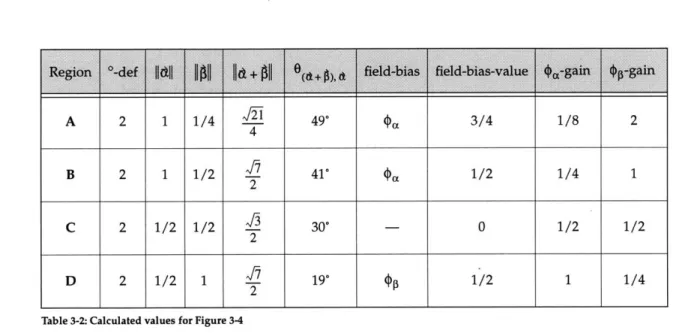
as it varies within IF and V,.3. Regions A, B, C, D denote those areas of [a e p bearing discrete I values.
These and other related values are documented in Table 3-2.
B 2 1 1/2 7 41' 1/2 1/4 1
2
C 2 1/2 1/2 30' - 0 1/2 1/2
2
D 2 1/2 1 19*$p 1/2 1 1/4
Table 3-2: Calculated values for Figure 3-4
Notes:
1. Region C field-bias-value is 0 as both d and
f
are of the same magnitude. 2. $a-gain = $p-gain in Region C as each field reinforces the other equally for reasons given above.1/8
2
2-4 3/4
3.5 EXAMPLES
CHAPTER 4
USE MODEL
Use ascriptions are made As seen in Chapter 2, fields interfere with one another. An arithmetic
to territories on the basis was defined on these fields in Chapter 3. This arithmetic tells either of
of theirfield structure. constructive or reductive interference. As shown below, it also sug-gests an assignment of use to certain field definitions.
Field structure is partitioned in three: go or directional structure, stop
or bi-directional structure and slack. A directional field structure is
termed a go structure as it reinforces direction and movement in that direction. A stop on the other hand is built by reductive field interfer-ence-no or little directional field bias is evident within the compos-ite field. Stops and gos are always relative to one another. A slack structure describes a relaxation in the degree of definition and rein-forces neither go nor stop.
Every elemental action is a go. As a result, designing use territories amounts to orchestrating field definitions; at times reinforcing gos with physical form, at other times building disjunctions in go systems for the purpose of stops or even slack.
This correlation of use and field structure is well defined. With the partition of the class of uses in three-access, relative privacy and col-lective-a mapping may be defined from use to field structure.1
1. The design of buildings as fish or binoculars may frustrate this claim.
4.1 ACCESS/GO DEFINITIONS
4.1 Access/go definitions
Access definitions are built with directional demarcations such that a principal field direction is reinforced. For instance, spatial extents X, P whose territories intersect and whose fields are parallel will strongly build access. Access need always be larger than its relative privacies.
4.1.1 Necessary and sufficient conditions for access/go field
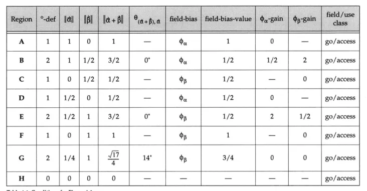
1. ||di + 01| > 1 2. 300 > 600 4.1.2 General conditions 1. See Table 4-1. A D H CF Figure 4-1
A 1 1 0 1 -- $a 1 0 - go/access B 2 1 1/2 3/2 0 $a 1/2 1/2 2 go/access C 1 0 1/2 1/2 - OP 1/2 - 0 go/access D 1 1/2 0 1/2 -a 1/2 0 - go/access E 2 1/2 1 3/2 0' $0 1/2 2 1/2 go/access F 1 0 1 1 - $0 1 - 0 go/access G 2 1/4 1 14' $P 3/4 0 0 go/access 4 H 0 0 0 0 - - - go/access
Table 4-1: Conditions for Figure 4-1
Notes:
1. Regions B and E display mirrored values for ||dl1, ||$||, field-bias, $ -gain
and $p -gain. There are also large field intensification values in
F,
Theseconditions are typical of parallelform. Passingform requires one additional con-dition: $,, , c ($, or $p).
2. Passing form can generate access or slack depending on the placement and
height of a and
P.
In region BE it is access as $ ( is uniformly 3/2i. If a and@
were further from one another or their height were less, then slack mightensue (cf Section 4.3).
4.2 PRIVACY/STOP DEFINITIONS
4.2 Privacy/stop definitions
Privacy definitions are built with directional demarcations such that one of two conditions obtains: there is no dominant field direction for
Va e P, (i.e. fields interfere destructively or are zeroed,) or there is a field reversal within 1a o P
-4.2.1 Necessary and sufficient conditions for privacy/ stop
field
1. Zeros: (field-bias-value Fa op) :) i/4, 600 > 1 >300 2. Reversal: (field-bias Fp) # (field-bias Va
s
4.2.2 General conditions
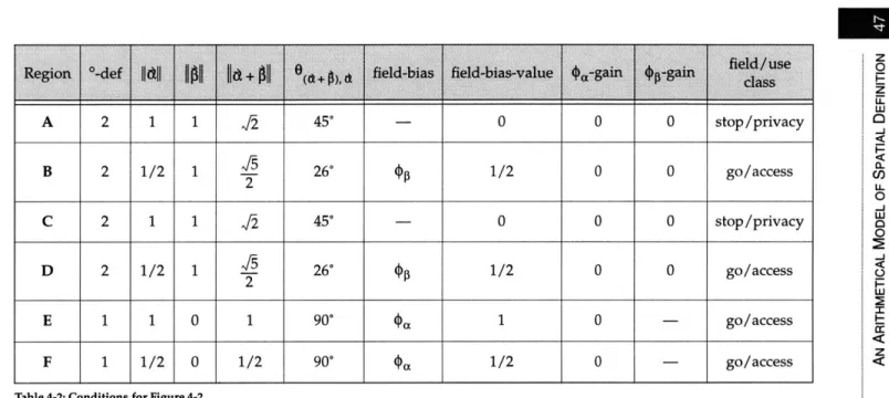
1. See Table 4-2.
E A B F
C D
Figure 4-2
B 2 1/2 1 26'$p 1/2 0 0 go/access 2 C 2 1 1 f2 45* - 0 0 0 stop/privacy D 2 1/2 1 26' 1/2 0 0 go/access 2 E 1 1 0 1 90* 1 0 - go/access F 1 1/2 0 1/2 90' Oa 1/2 0 - go/access
Table 4-2: Conditions for Figure 4-2
Notes:
1. Regions B, D are identical in all respects. This is characteristic of Tform, as
is the field reversal across regions BF, DR (Field reversal occur when field-bias-values change across contiguous territories.) As 0 moves further from
a, the reversal diminishes. As
s
moves closer to a, the reversal may bereplaced by a zeroing, wherein the field-bias is nil. The same reasoning
applies for a with respect to
P.
2. Regions A, C are also identical in all respects as expected of Tform. They
both display a field-bias of 0, and requisite 0 + ) value.
3. All regions exhibit 0 valued field intensifications. This occurs if and only
if $a and $p are normal to one another as in this example.
4.3 COLLECTIVE/SLACK DEFINITIONS
4.3 Collective/slack definitions
Field definitions may vary in their degree of definition. Where there is a relaxation in the degree of definition, one finds slack. Slack regions support collective uses and even the encroachment of neigh-bouring uses without forfeiture of overall organisation.
4.3.1 Necessary and sufficient conditions for collective/ slackfield
1. fields with degree-def > n flank some definition of degree-def = n
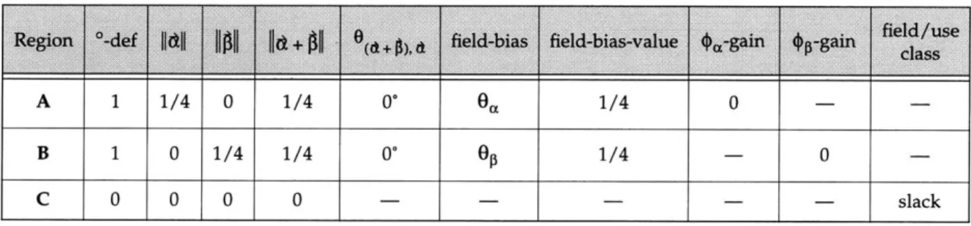
2. size of the slack zone is at least that of its flanking territories. 4.3.2 General Conditions 1. See Table 4-3.
S
A
C) Figure 4-3z
o
UA 1
LI-C0
Redi on + + + field-bias field-bias-value $.-gain $Zgain a
L
A 1 1/4 0 1/4 0 0a 1/4 0
B 1 0 1/4 1/4 0" 0p 1/4 - 0 -a
C 0 0 0 0 - - - slack
_-J
Table 4-3: Conditions for Figure 4-3
i-J
Notes:
1. Figure 4-3 shows F, and IF disjoint and of degree-def = 1. Between them Z
is a zone of degree-def zero-hence an alternation in definitions. This slack
zone is not, strictly speaking, a territory as there is no field definition.2
2. Regions A, B are neither stops nor gos. The field definition is too weak for a
go and 0 is too small for a stop.
3. As slac is
df
a lesser degree of definition it most often belongs to a larger sized territory which a and $ have partially intensified. As a vestige of the larger definition, slack plays an important role; it allows concurrent territorial associations across sizes.2. This is not entirely true. Appendix A shows that cc and 0 induce a territory owing to dimensional stability.
4.4 CASE STUDIES
4.4 Case Studies
4.4.1 Access/Go
4.4.1.1 Bazaar Road: Chitral, Northwest Frontier Province, Pakistan
Figure 4-4
A
Figure 4-5
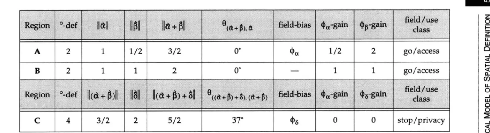
Parallel shop fronts produce a strong directional field occupied by access. This field, $,, is further intensified by a covered walk. The shops themselves reverse $a owing to their great depth. This results in relative privacies or stops. See Table 4-4 for computed values.
A 2 1 1/2 3/2 0' $a 1/2 2 go/access
B 2 1 1 2 - 1 1 go/access
Region *-def
||(d
+
)||01 |1(d
+0)+
+ 8ge
( +
field-bias $a-gain $5-gainfield/use
C 4 3/2 2 5/2 37' $6 0 0 stop/privacy
Table 4-4: Conditions for Figure 4-4 and 4-5
Notes:
1. Very large
Id
+ 0|| suggests access in region B.2. Region A also displays large If and serves pedestrian access.
3. Region C shows a stop. This corresponds with the anteroom of stores. 4. Region D displays a field reversal in $a .This area forms the back rooms for shops.
4.4 CASE STUDIES
4.4.1.2 Gale House: Frank Lloyd Wright
Figure 4-6a/4-6b
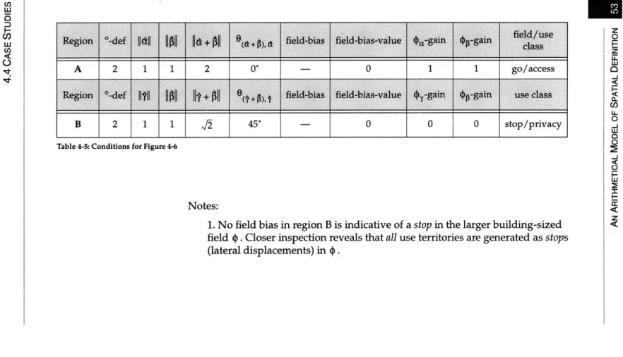
Walls a and p reinforce the building sized field <p and build an access zone I' 6 .Note that
s
passes a, thus simultaneously contributing to the stop definition I0 *See Table 4-5 for computed values.
A 2 1 1 2 0" - 0 1 1 go/accessI
2 1 1 f2 45' 0 0 0 stop/privacy
Table 4-5: Conditions for Figure 4-6
Notes:
1. No field bias in region B is indicative of a stop in the larger building-sized
field $. Closer inspection reveals that all use territories are generated as stops (lateral displacements) in $.
4.4 CASE STUDIES
4.4.2 Privacy/Stop
4.4.2.1 Verandah, Village of Taqma, Salang Mountains, Afghanistan
otx
Figure 4-7
Wall element a induces a strong directional field to which access has been assigned. This direction is reinforced by
P
and sectional access S. The lateral displacement of P weakens *a e p allowing for y to gener-ate a full stop, , 9 (a aP)
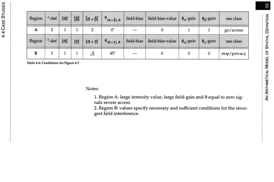
.As expected of field stops, a relative privacy is built-in this case a summer kitchen.See Table 4-6 for computed values.
w
5Z
Region dId
t-def
+ field-bias field-bias-value $a-gain $-gain use classC/) Zk
A 2 1 1 2 '- 0 1 1 go/access
-j
Region 0-def
ll
it|
+|d +| + ), field-bias field-bias-value $a-gain $,-gain use class
a-C')
L-B 3 1 1 f2 45' - 0 0 0 stop/privacy 0
w
Table 4-6: Conditions for Figure 4-7 0
|-w
Notes:
1. Region A: large intensity value, large field-gain and 0 equal to zero sig- Z
nals severe access
2. Region B: values specify necessary and sufficient conditions for the stron-gest field interference.
4.4 CASE STUDIES
4.4.2.2 Gale House: Frank Lloyd Wright
Figure 4-8a/4-8b
Walls a and y, build a go definition
Fa
ey.
Fireplaces
and closure 8 introduceT,
9 8 with $p 9 8 normal to $ae
y .These opposing fieldslead to a zeroing at r(s a ) a (a ) y) -sufficient to build a privacy
which is clearly in evidence by use. Note that slack is built between territories ABCD and I, denoted by EFGH.
See Table 4-7 for computed values.
5/4 5/4 52 B 4 1 5/4 38' 1/4 stop/privacy C 4 5/4 5/4 52 * - 0 stop/privacy D 4 1 5/4 38" 00+8 1/4 stop/privacy E 3 1 1/2 65* $4,9 1/2 go/access F 3 5/4 1/2 68* 3/4 go/access G 3 1 1 1 90' - 0 go/access H 3 5/4 1 51* 1/4 stop/privacy I 4 5/4 0 J5 90' 5/4 go/access
Table 4-7: Conditions for Figure 4-8
Notes:
1. Region EFGH is slack as it is flanked by territories of greater degree-def.
2. Region EFGH is also rendered as access.
stop/privacy CO) w 5 w ...
4.4 CASE STUDIES
4.4.3 Collective/Slack
4.4.3.1 Hysolar Institute, Universitdt Stuttgart: Ginter Behnisch
-0E
Figure 4-9
Between
Fa
and 15 exists a territory of roughly equal size and of degree-def less than bothF,
and F,. As expected, this slack zone accommodates collective use, and allows for association with larger sized definitions (site and landscape).4.4 CASE STUDIES
4.4.3.2 Village of Kolalan, Koh Daman Valley, Afghanistan
Figure 4-10
Slack zones are dearly in evidence at varying sizes. The uses ascribed to these are always public.
4.4.3.3 Fallingwater (ground floor): Frank Lloyd Wright
Figure 4-11
The site's directional field is built by the sectional element a and Bear Run Creek. Wright reinforces this directional field through the regis-tration of elements shown by horizontal bands. Those elements shown by vertical bands build an opposing directional field which forms variable zeros and reversals. The territories exhibiting these zeros and reversals are occupied as relative privacies. Note the slack in zone H, thus reinforcing association at the largest (landscape) size.
AN ARITHMETICAL MODEL OF SPATIAL DEFINITION 4.4 CASE STUDIES
A
A' 2 1.45 20' vertical band go/access
B 2 2.00 0' vertical band go/access
C 3 1.60 38* horizontal band stop/privacy
D 4 1.41 45' - stop/privacy
E 4 1.95 56* horizontal band stop/privacy
F 4 1.95 56' horizontal band stop/privacy
G 4 1.6 39' horizontal band stop/privacy
H 2 1.25 0' - go/access/slack
I 4 4.00 45' - stop/privacy
Table 4-8
Notes:
1. An important component in the generation of the slack zone H is the screen
assembled from two principle columns. Appendix A illustrates the manner in which territorial control assembles these columns into the larger sized defini-tion of a screen.
4.5 SIZE
4.5 Size
Very little mention has been made of particular use sizes. This has been deliberate as go, stop and slack behaviours can be found at all sizes. They operate across sizes as well, though these are limited to interactions with the next larger and smaller size.
The foregoing has been content to describe privacy, access and collec-tive in purely relacollec-tive terms. Of course in the full determination of use, reference must be made to size. Introducing size as an additional condition to those of Sections 4.1, 4.2 and 4.3 is sufficient for this pur-pose.
Table 4-4 ranks the seven major sizes within which architectural form most commonly operates. Each size accommodates access at that size.
material < 3' personal 3-8' room 8-14' collective 14-25' building 25-100' site 100'+ landscape 200'+
access at each of the sizes above Table 4-9
CHAPTER 5
CONCLUDING REMARKS
The arithmetical model sketched in Chapters 2 and 3 found applica-tion in the use model of Chapter 4. Other investigaapplica-tions of architec-tural form lend themselves to the model. Several are suggested below.
5.1 Other applications
5.1.1 Form families and organisations
Some generic form organisations such as the Tform, parallelform and
passingform were identified in terms of their shared territories' field
structure (Tables 4-1, 4-2). Other form families should be as easy to describe. One advantage of describing these in terms of their territory is that the particularities of the physical form (outside of the determi-nation of its spatial extents) need never be addressed. Form is
under-stood as an organisation, not shape.
5.1.2 Containment
Containment can be expressed as a function of degree of definition and field intensity. The greater the number of inducers and intensity of their resulting territories, the greater the containment.
5.1 OTHER APPLICATIONS
5.1.3 Light
Just as territories have been said to be built by physical demarcations, so too is light. The definition of spatial extents, particularly as applied to ensembles, describes the building of light. (See Section 4.4.3.3 and Appendix A.)
5.1.4 Computational model
The spatial model's scope of applicability and mathematical formali-sation invites computational implementation.' Analytical engines might map the territorial commitments of any architectural form. Knowledge-based systems such as that proposed by Koile (1997) may reason with these computed territories.
Alternatively, application programs may allow for user interaction at the level of territory; given a desired territorial definition, the applica-tion informs the user of those physical form properties necessary for its inducement. Note that in this last case the mapping from territory to physical form is not injective; uncountably many instances of physical form can build a particular territory.2
1. Appendix B diagrams a set of Classes and Methods for the arithmeti-cal model of spatial definition presented herein.
2. The interest in building application programs to generate physical form is wrong-headed. At best its results will remain uninteresting as arbitrary rules of shape are introduced to limit that which is
unbounded. The far more interesting and difficult question is: what spatial understanding gives rise to desired properties of physical form, and how does the latter accommodate the former.
5.2 CONCLUDING REMARKS
5.2 Concluding remarks
Spatial definition admits to an infinitude of articulations; material, light, use, dimension, tectonics and sundry combine in rendering ter-ritory. Given the many properties of which it is comprised-and pre-sumably manners in which it is defined-there would appear little hope of saying much more (or less) than has been said by countless others.
In response, this model of spatial definition reduces the aforemen-tioned infinitudes to a modest three: dimension, direction and inten-sity. Those manners by which territory is induced are reduced to one: the projection of physical form's spatial extents. Though the abstrac-tion dispenses with much of the phenomenological, it remains firmly rooted in experience-not as a model of experience, but one informed by the same.
The arithmetical model of spatial definition presented herein makes precise hypotheses of the empirical world. No doubt these will soon shipwreck upon the large and dispassionate world of empirical fact, and take with them these 82 pages. However the method which invited the formalisation-one which Jerome Wiener had once described as 'represent[ing] nothing less than the good manners of
5.2 CONCLUDING REMARKS
the mind'3-will survive the errors of this work; as it will survive the charlatans of Heidelberg; as it will the sophists heralding 'new archi-tectural promenades.'
May architecture, and those whom it is to serve, fare as well.
3. Communicated to the Department of Architecture on February 14, 1963 when serving on the MIT Visiting Committee to the School of Architecture and Planning. (Told the author by M K Smith).
APPENDIX A
E N S E M B L E S
Necessary and sufficient The spatial and arithmetic models of Chapters 2 and 3
accommo-conditions are considered dated ensembles as though they were any other form of like spatial
for the determination of extents.
ensembles.
In experiencing architecture our understanding takes seemingly dis-parate elements and fashions them into coherent assemblies-much as does the mind with discrete notes of music, building harmonic, melodic and contrapuntal assemblies from them. What properties of form are addressed in constructing these architectural assemblies? There are any number, to be sure. One class may be described as physical attributes, which includes material, colour, dimension and tectonic type. Another class of properties may be termed formal, which includes spatial organisation. These are present at all sizes.
Physical attributes build ensembles through association; elements are grouped on the basis of shared properties. Elements in concrete may be deployed in such a way that the material builds associations at the building size. A secondary structure, if made legible, would consti-tute an association at a smaller size than the primary structure. Repeated use of dimension, or material might allow for the assembly of a screen, a structural bay or village and so on. For the most part, a class as this would tie the elements together by virtue of shared intrinsic properties, and cast the ensemble as the extents of those ele-ments.
Spatial organisation performs somewhat differently. The association built is not through a shared physical property, but a spatial organisa-tion in which each element is a necessary part. For instance a set of columns may be read or assembled as a bay by virtue of the columns' spacing and height. Similarly, a piece of landscape may be claimed through a dimensional displacement at a building size. This appen-dix considers only those ensembles built from spatial organisation. It describes necessary and sufficient conditions for an organisationally built ensemble.
Evidence of spatial organisation can be found in the constituent ele-ments' mutual control of shared territory. If Fa e
s
exists for some ele-ments A and B, then A and B control one another as each intensifies the other's territory in IF e p .Spatial organisation can also be found in the consistent dimensional deployment of elements. If an element's dimensions are also recorded in its placement vis-a-vis other ele-ments, then a recognisable association is made, one which is termedself-stability. Each will be treated in turn.
Definition: Consider elements A and B and their respective territories
Fa and
TF
p. An ensemble builtfrom
territorial control is the set ofinduc-ers for a e p such that:
1.T 0p#
2. i ||d|| 2 i/2 in region (A ( B) i 1
|||
1 i/2 in region (A ( B)(min (size a)(size
p))
(size r ) (-(min (size a)(sizeP))1)
4. ||d||= 11 ||
The rationale for the definition is as follows:
Condition
1
ensures that p exists. Recall that a necessary con-dition of an ensemble is that its constituents participate in the control of one-another's territory.Condition 2 ensures that Ia p occurs where
Fa
and Fp are strongly defined. Ifra
e p were elsewhere inF
and I7p, the mutual territorial control would be too weak to register expe-rientially.Condition 3 ensures that Fa D P is not trivially small nor large.
Condition 4 ensures that a and
P are roughly equal in their control
of the other's territory.
In sum, one might claim that our reading of Fa
e
p acknowledges the inducers and joins them in experience. Examples are given in Sections A.0.1 and A.0.2.Definition: An ensemble built from dimensional stability is one in which
for elements A, B the element A is displaced its own dimension from B. An example is given in Section A.0.3.
It is important to note again the manner in which these ensembles generate their territory as ensembles. The territory generated by these ensembles is simply that given by the projection of their extents. The
only quantitative difference between the territory associated with a structural bay element and a wall element, say, is that the bay's pro-jection of extents renders a footprint of usable territory, whilst the
wall yields a footprint occupied by material.
A.0.1 Study: Ensemble built from territorial control: screen definition in
Fallingwater (ground floor)
Figure A-1
Figure A-1 depicts F,,, ]F and Fa e p. The following conditions obtain:
1.
Fae,
is non empty and occurs where I fa and If, are greatest. 2. Region M assumes the maximum If value for ra u Vp. HenceFa e P is extrinsically controlled.
3. M is at least of size a and
p.
4. ||d||
lIll
in region M.
All four conditions obtain for a and
P
to build an ensemble a. In Figure A-2 below, the spatial extents and resulting territories for ap are drawn. Note that these extents partake in slack and stop defini-tions described in Chapter 4, Section 4.4.3.3.Figure A-2
It should be noted that column a and the fireplace do not form an ensemble as condition 3 fails.
A.0.2 Study: Ensemble built from territorial control: the Ha of Hunza
Val-ley, Northern Areas, Pakistan
The ha is the most important room in the domestic architecture of the Hindu Kush and Karakoram of Central Asia. A room of approxi-mately 20' x 17' need accommodate: women's sleeping quarters, men's sleeping quarters, a place for musicians, a kitchen and storage.
Figure A-3
Outside of its four walls, the only physical form present is that of four posts. Because of their height and spacing, an organisation obtains which is akin to that seen in Fallingwater. Applied four times over, the requisite spatial definitions are made. These are illustrated in Figure A-4.
Figure A-4
Regions M, S, T, Y boast the largest If values for their respective col-umns. As conditions for an ensemble are met for each pairing, four ensembles are built. (In point of fact, these very ensembles build a fifth ensemble which is that of the four column bay.) NEW Territories are built with every ensemble.
Note that the columns do not form diagonal pairings. This is a result of their geometry (their spatial extents do not project diagonally) and height and spacing (conditions 2 and 3 above fail).
A.0.3 Study: Ensemble built from dimensional stability: Parliament
Build-ing, Bonn, Deutschland, Gunter Behnisch
Figure A-5
Lines denote dimensions of various elements. Note that the elements responsible for these dimensions are in turn displaced from other physical demarcations by the same dimension. Territory is built with-out resort to a strict, hierarchically arranged plan.
APPENDIx B
CLASSES AND METHODS
wall partition
r
screen column ensemble slots: component-elements 'architectural-element slots: physical-form territory-form 'geometric-form slots: geornetry-object methods: direction centre of gravity size-label 'geometry-object slots points height 'use-form slots: methods: 'field-form slots methods: edesign-obje slots: methods: physical-form slots: t territory-form slots. i material colour ectonics nducers field-form methods: degree-def control territories size-label use-label inducers direction bias bias-value intensity-value architectural-elements use-formsterritory-forms (note: collected from architectural elements)