Assessment of a compact steam generator aided by computational fluid dynamics

Assessment of a Compact Steam Generator Aided

by Computational Fluid Dynamics

by

Brandon Ariel Aranda Ocampo

Submitted to the Department of Nuclear Science and Engineering

in partial fulfillment of the requirements for the degree of

Bachelor of Science in Nuclear Science and Engineering

at the

MASSACHUSETTS INSTITUTE OF TECHNOLOGY

May 2020

© Massachusetts Institute of Technology 2020. All rights reserved.

Author . . . .

Department of Nuclear Science and Engineering

May 08, 2020

Certified by. . . .

Koroush Shirvan

Assistant Professor, Nuclear Science and Engineering

Thesis Supervisor

Accepted by . . . .

Michael Short

Class of ’42 Associate Professor of Nuclear Science and Engineering

Chairman, NSE Committee for Undergraduate Students

Assessment of a Compact Steam Generator Aided by

Computational Fluid Dynamics

by

Brandon Ariel Aranda Ocampo

Submitted to the Department of Nuclear Science and Engineering on May 08, 2020, in partial fulfillment of the

requirements for the degree of

Bachelor of Science in Nuclear Science and Engineering

Abstract

Steam generators are an essential component in nuclear power plants which serve to transfer thermal power from a liquid coolant to steam by boiling water. Even with many advancements in the designs of steam generators, they still require extremely large sizes and have high costs which are major hurdles for the implementation of new reactor designs such as Small Modular Reactors. Using a Printed Circuit Heat Exchanger (PCHE) such as those from the company HeatricTM as a steam genera-tor to boil the liquid in the secondary side has potential to overcome the disadvan-tages of conventional steam generators. Computational Fluid Dynamics was used to aid the assessment of such compact steam generator. The models used were bench marked against a 1-D MATLAB code which simulated a compact steam generator with straight, semi-circular channels. The same conditions were used to simulate a zig-zag, semi-circular PCHE. The zig-zag configuration resulted in a 22 ∘𝐶 increase in superheat over the straight channel configuration at the cost of pressure drops that are over 4 times higher but yet easily accommodated. The PCHE was also simulated in different orientations with respect to gravity and determined there is little advan-tage in using a vertical layout regarding pressure drop for the zig-zag configuration. Plugging of a single channel was also simulated to determine the effect on surrounding channels and potential hot spots.

Thesis Supervisor: Koroush Shirvan

Acknowledgments

First I would like to thank Professor Koroush Shirvan for taking me on to his team and guiding me throughout the entire project. Professor Shirvan provided me with constant support and was always ready to help me when I needed it. Completing this project without any prior knowledge of CFD was a major battle and he was always extremely patient and strived to ensure I always learned from the project. I am thankful to have had him as a mentor through this project and for all the knowledge and advice he has shared with me.

I would like to thank those that gave me guidance on the process of completing this thesis. Thank you to Professor Paola Cappellaro for sharing her wisdom and putting me on the right track to begin and complete my thesis. Thank you to Jared Berezin for all the guidance he has given while writing this thesis and in previous classes.

I would also like to thank the faculty that have helped me throughout my years at MIT and provided me with countless advice as I journeyed through unknown territory. Thank you to Professor George Barbastathis who mentored me and was always there to guide me. Thank you to Professor Michael Short who provided me with my first ever opportunity to perform research and who has given me advice on my path countless times.

Thank you to all my friends whom have supported me and encouraged me every step of the way. I am thankful to have been able to make many amazing friends and join an amazing community since the start of my time in college. Being the first person in my family to go to college was scarier than I could have ever imagined and they have made it an experience to always remember. I am also thankful for the friends from home that have been there since the beginning and that have continued to support me even as I build my life in a new world. A special thank you to my partner that has been extremely supportive, caring and comforting throughout this entire process and more.

this goal I would never have imagined myself completing. My parents have been the biggest supporters I have had and have always done everything they could to ensure my success. Even when I questioned my ability to succeed in college, they encouraged me and cheered me on. They have given up more than I could ever ask for to help me be where I am today. This degree pales in comparison to all they have done to come to the United States and all they have gone through. I hope this degree culminates the journey that they started long ago.

Contents

1 Introduction 13

1.1 Motivation . . . 13

1.2 Previous Work . . . 15

1.3 Objectives and Methods . . . 15

1.4 Outline . . . 16

2 Background 19 2.1 Steam Generators . . . 19

2.1.1 Use in Nuclear Reactors . . . 19

2.1.2 Disadvantages of U-Tube Steam Generators . . . 19

2.2 PCHEs . . . 21

2.2.1 Design and Manufacturing of PCHEs . . . 21

2.2.2 Applications of PCHE . . . 22

2.2.3 Nuclear Applications . . . 23

2.3 Uncertainty in Boiling Correlations . . . 23

3 Benchmarks 25 3.1 Introduction . . . 25

3.2 Friction Factor Simulations . . . 25

3.2.1 Straight Pipe . . . 26

3.2.2 Semi-Circular Wavy Channel . . . 27

3.3 Heat Exchanger Simulations . . . 30

3.3.2 Model and Conditions . . . 30

3.3.3 Results . . . 32

4 PCHE Steam Generator Modeling 35 4.1 Introduction . . . 35

4.2 Straight Channel PCHE Boiling . . . 36

4.2.1 Model and Setup . . . 36

4.2.2 Determining Coefficients for the Rohsenow Correlation . . . . 37

4.2.3 Sensitivity Study . . . 41

4.2.4 Orientation of PCHE With Respect to Gravity . . . 43

4.3 Zig-Zag Channel PCHE Boiling . . . 44

4.3.1 Model and Setup . . . 44

4.3.2 Boiling Results With Single Channel Periodicity . . . 46

4.3.3 Changing Orientation of Gravity . . . 50

4.3.4 Plugging of a Single Channel in Secondary Side . . . 51

5 Conclusion 55

List of Figures

2-1 A steam generator replacement for the Callaway nuclear plant . . . . 20

2-2 Plates of a PCHE from HeatricTM _{. . . . 21}

2-3 A PCHE from HeatricTM _{in cross-flow configuration . . . . 22}

3-1 The mesh generated for the simulation of the pressure drop in a straight pipe. . . 26

3-2 Friction factor in a straight pipe over a range of Reynolds number. . . 27

3-3 Geometry of the semi-circular wavy channels with a diameter of 2 and wavelength-to-width ratio of 7. . . 28

3-4 The friction factor in a semi-circular wavy channel with a diameter of 2 mm and wavelength-to-width ratio of 7. . . 29

3-5 The friction factor in a semi-circular wavy channel with a diameter of 1.2 mm and wavelength-to-width ratio of 30. . . 30

3-6 Cross section of PCHE from TiTech . . . 31

3-7 Mesh of the PCHE from TiTech with CO2 and water . . . 33

4-1 Geometry of the straight channel PCHE steam generator . . . 36

4-2 Mesh of the single set of channels in straight PCHE . . . 38

4-3 Mesh 2 of the single set of channels in straight PCHE . . . 42

4-4 Vapor fraction in the y-z plane of the channel of boiling water in a (a) horizontal configuration and (b) vertical configuration . . . 45

4-5 Geometry of the zig-zag channel . . . 46

4-6 Mesh of the single zig-zag channel . . . 46 4-7 Volume fraction of vapor in the secondary side in the zig-zag PCHE . 47

4-8 Surface average temperature along the z-direction of the heat exchanger of the two fluids . . . 48 4-9 Model of multiple channels with a single channel in the secondary side

filled with air . . . 52

A-1 Polynomial fits of the density of supercritical CO2 at 8 MPa split into

List of Tables

3.1 Geometry of the semi-circular wavy channels for pressure drop simu-lations . . . 28 3.2 Design of the PCHE from TiTech . . . 31 3.3 Inlet conditions for TiTech PCHE Simulation . . . 32 3.4 Simulated versus experimental outlet temperatures and pressure drops 34

4.1 Properties of the semi-circular PCHE boiling model . . . 36 4.2 Outlet temperatures and pressure drops for varying coefficients in the

Rohsenow correlation . . . 39 4.3 Comparison of meshes used in straight channel boiling . . . 41 4.4 Outlet temperatures and pressure drops for mesh sensitivity study . . 42 4.5 Comparison of results from different turbulence models . . . 43 4.6 Outlet temperatures and pressure drops in different orientations . . . 44 4.7 Comparison of outlet temperatures and pressure drops from boiling in

a straight and zig-zag PCHE . . . 47 4.8 Heat transfer coefficients times the heat transfer area of the different

regions in the PCHE . . . 50 4.9 Outlet temperatures and pressure drops from boiling in a vertical PCHE 51 4.10 Outlet temperatures and pressure drops in the channels surrounding

the plugged channel . . . 53 4.11 Temperatures in the plugged channel . . . 53

Chapter 1

Introduction

1.1

Motivation

The construction of nuclear reactors has seen a large decline in recent decades in western countries with most of the current operational reactors having been built between 1970 and 1990 and very few being built ever since [1]. This is due in large part to the high initial costs required to build large nuclear reactors that also satisfy all the safety standards in place today. The fission reactors in use are large systems with multiple components that require years of construction and lots of costly material to be built. One of the largest subsystems of a nuclear reactor that is critical to the operation and dimensions of a fission reactor is the cooling system. The cooling system is composed of large heat exchangers such as the steam generators present in Pressurized Water Reactors (PWR). Some steam generators which use shell designs such as the shells for the Hanford steam generators can be longer than 60 ft and have diameters over 10 ft [2].

Recently, there has been a lot of interest in creating Small Modular Reactors (SMR’s) that would have the advantage of being cheaper to produce with shorter construction timelines. These SMRs are also appealing as they can then be inte-grated together to create larger power plant systems to fulfill power requirements as the infrastructure grows, such as in developing countries [3]. Smaller organizations interested in entering the energy market which is known for its high initial cost would

now be able to do so by acquiring SMRs which would decrease the time to pay off the cost of starting such a power plant. This movement towards SMRs and the interest of expanding the nuclear energy market has sparked a movement to create new reac-tor designs and optimize the components currently in the reacreac-tors with the goal of developing smaller and simpler concepts. Reducing the size of the heat exchangers, one of the largest components in a rector, would be one of the biggest improvements that could be made towards reducing the size of fission reactors and could kickoff the start of the implementation of SMRs.

Heat exchangers are the most commonly used cooling systems for large scale ap-plications and can be found in all types of power plants and even in other industries. Many companies and institutions have dedicated themselves to the research and opti-mization of heat exchanger designs to improve efficiency and heat transfer capacities while also attempting to maintain or decrease the size. The current trend is toward the design of compact heat exchangers (CHE’s) which use smaller channels than con-ventional heat exchangers which increases the heat transfer capabilities. The company HeatricTM _{has been one of the most successful in the area of CHE’s with the printed}

circuit heat exchanger (PCHE) that they have designed. PCHE’s have high promises for delivering the necessary heat transfer capabilities along with the reduced size that are required for SMR’s. Unfortunately, few technical details have been released by the company which limits the ability to accurately model and implement them within reactors, leaving a need for analysis on these PCHE’s, specifically in using them as steam generators.

Steam generators are typically used in nuclear reactors to boil water into steam which can then be used to drive turbines to generate electricity. Much of the focus of the push towards SMRs is on reducing the size of these steam generators. There has been a particular interest in using PCHEs as steam generators since their compact size and high power density is attractive for boiling water. Further research is required to verify the ability to use a PCHE as a steam generator and determine the potential problems that could arise from such use.

1.2

Previous Work

Previous work has attempted to model the PCHE’s from HeatricTM _{and develop}

correlations for others interested in using a PCHE. For example, Von Meter attempted to reverse engineer the geometry of the channels of a PCHE from HeatricTM _and

modeled heat transfer between water and supercritical carbon dioxide in such PCHE using Computational Fluid Dynamics [4]. Computational Fluid Dynamics (CFD) has been used as a simulation tool to predict the performance of these compact heat exchangers when designing them for new applications and has also been widely researched and developed. However, most of this research done for the PCHE’s have only modeled single-phase heat transfer and little work has been done to model two-phase heat transfer. The research that has been done for two-two-phase heat transfer so far has only focused on large channels with diameters larger than 5 mm and microchannels with diameters smaller than 0.5 mm. Channel sizes in between 0.5 and 5 mm have an opportunity to be highly efficient and could lead to further reduction in the size of the steam generators for use in the SMRs. This research project will use CFD simulation tools to aid in the computation of the performance of compact steam generators with channel diameters in the region of 0.5-5 mm for implementation in SMRs.

1.3

Objectives and Methods

The main goal of this research project is to simulate and predict the boiling and creation of steam in the secondary side of a PCHE that would be coupled to the primary side of a nuclear reactor. This involves finding the outlet temperatures of the two fluids, pressure drops, and many other properties. The simulations will be conducted for semi-circular channels with straight and zig-zag geometries to compare the performance of the two configurations. Additional simulations will be performed in which some channels are plugged to evaluate the effect on the performance.

Dy-namics software and the theory behind it. The software used was Star CCM+ from Siemens. After the author gained confidence in using the software, pressure drop simulations done by Gezelius were recreated to test the skills of the author and gain knowledge as similar geometries would be used in the project [5]. Similarly, simula-tions carried out by Von Meter for the use of PCHE to transfer heat from supercritical carbon dioxide to water were recreated to compare the results and validate the abili-ties of the author. Once the skills and results of the simulations were validated, the PCHE model was used to simulate the boiling of the water in the secondary side from the heat transfer of the water in the primary side. This simulation would be an ad-ditional contribution to estimate the performance of the PCHE as a steam generator in addition to the 1D-simulation code from Shirvan used in the paper from Haratyk, Shirvan and Kazimi [6].

Once the simulations are tested and valid results are obtained, changes in design will be made to test the impact on performance. A single channel will be left empty to test the effect on the local temperature around the channel. Multiple channels will also be tested. Pressure drops and other properties will be evaluated to determine whether the changes will benefit the overall performance without inducing any further complications.

1.4

Outline

Chapter 1 gives a brief overview of the research topic along with the goals and benefits of this project.

Chapter 2 provides the background needed to understand the advantages and disadvantages of current steam generators. A description is given on PCHEs and their advantages and their potential for use as steam generators. The uncertainty of boiling models currently used will also be discussed.

Chapter 3 contains the benchmark models and tests that were simulated to be compared to previously obtained results. One important benchmark is that of the 1D-simulation created by Shirvan. The final task is an extension of this model with a

zig-zag configuration which would also be tested under different conditions so agreement with such benchmark was critical for continuing the work.

Chapter 4 presents the final models and results for evaluating the performance of the zig-zag PCHE used as a steam generator in the different conditions. Qualita-tive and quantitaQualita-tive analysis is performed to determine the benefits and potential problems associated with its usage as a steam generator.

Chapter 2

Background

2.1

Steam Generators

2.1.1

Use in Nuclear Reactors

The majority of the nuclear reactors that have been built are Boiling Water Reactors (BWR) and Pressurized Water Reactors (PWR) which use water to cool the core of the reactor where the fuel is held. These reactors have thermal power outputs on the order of thousands of megawatts (MW) such as the Westinghouse 4-loop PWR which has a gross thermal power output of 3400 MW𝑡ℎ[7]. To convert this thermal power to

electric power that can be used, PWRs use a secondary fluid which is usually water that is boiled through u-tube steam generators coupled with the fluid in the primary side [8].

2.1.2

Disadvantages of U-Tube Steam Generators

While u-tube steam generators can be designed to be very efficient, their downside is their large size required to boil the water. The size of a u-tube steam generator can be seen in figure 2-1 which shows the replacement steam generator for the unit 1 Callaway nuclear plant [9]. The steam generator pictured measured 68 feet tall and 17 feet in diameter and weighed 372 tons [9]. The size of the steam generators is a major factor that drives the size and cost of the reactor when it is being built and designed.

Since these steam generators are made of many components with multiple interfaces, there exists many points of failure that need to be considered when designing the reactor. Extra safety features need to be included to account for these potential accidents such as ruptures in the steam generator’s tubes. All those safety features that are ultimately included in the reactors drive up the prices even more.

Figure 2-1: A steam generator replacement for the Callaway nuclear plant [9]

Many of the problems that can arise from steam generators are usually related to the challenges of supporting the thousands of tubes that are wound throughout the steam generators [8]. Maintenance and inspection of these steam generators proves to be a difficult task with such large amounts of tubes. One large concern for these tubes is the degradation of the tubes due to the chemicals used in the water which leads to the thinning of tube walls [10]. Eventually, the damage on these tubes can cause them to fail which can potentially be economically disastrous. For example, the San Onofre was forced to shut down after it was found a new steam generator was defective due to the flow interactions with the tubes and tube sheets [10]. Even if a plant is not forced to shut down, they will likely have to replace the steam generators which can be extremely expensive. The steam generator replacement project for the David-Besse nuclear plant which replaced two steam generators along with some other upgrades cost $600 million [11]. These high maintenance costs and the high risk of

steam generator failures contributes to the deterrence of construction of new nuclear power plants. Particularly, many small reactors encapsulate the steam generator within their reactor vessel, requiring larger and stronger vessels which are a very expensive component of a nuclear reactor. Therefore, identifying more compact and resilient solutions to steam generator design are of importance for the requirements of the next generation reactors.

2.2

PCHEs

2.2.1

Design and Manufacturing of PCHEs

The PCHEs developed by Heatric TM _{are different from normal heat exchangers in}

that they are composed of plates with mini channels which are bonded together. The typical design of a PCHE is of zig-zag channels with a semi-circular cross section having a diameter of 2 𝑚𝑚 [12]. The zig-zag configuration is shown in figure 2-2 which contains two plates that would be bonded together [12]. The PCHEs are usually used in counter-flow configuration but can also be used in cross-flow configuration. Figure 2-3 shows a PCHE that has been assembled for cross-flow configuration with two channels for one side to each channel on the other side.

Figure 2-2: Plates of a PCHE from HeatricTM [12]

The zig-zag design of the PCHE is a feature that is meant to enhance the heat transfer between fluids. Thanks to the zig-zag design and the small size of the

chan-nels, the PCHE is able to reduce the size and weight up to 85% compared to shell and tube heat exchangers [12]. This is extremely beneficial for applications in which the size of the heat exchanger needs to be minimized.

Figure 2-3: A PCHE from HeatricTM in cross-flow configuration [12]

The PCHE’s are composed of multiple sheets of metal with the fluid channels chemically etched into the material. The sheets are joined through a process named diffusion bonding which occurs at high temperatures and causes the grains of the metal to grow between plates [13].The result of this manufacturing process is a heat exchanger with the strength of the parent material as the diffusion bonding process does not produce any interfaces or other potential failure points [12]. These PCHE can operate at temperatures up to 800∘𝐶 and pressures up to 500 𝑏𝑎𝑟 [13]. The small fluid channels result in larger surface areas for heat transfer per volume of the heat exchanger which results in its high power density. This makes them an attractive choice for many applications with single-phase flow.

2.2.2

Applications of PCHE

The PCHE was first commercialized in 1985 with its focus being on industrial re-frigeration systems [13]. Currently, they are most commonly used in the offshore industry and more than 500 PCHEs have been commissioned since 2001 [13]. While the upfront cost of the PCHE may be higher than other heat exchangers such as the Brazed Aluminum Heat Exchangers which is used by some gas producers, their high durability allows them to bring higher returns due to the lower maintenance and

repairs required throughout their lifetime [14]. Research has been conducted for the application of a PCHE for reactors such as heterogeneous catalytic reactors and there is interest in many other industries with a variety of fluids [13].

The manufacturing process of HeatricTM _{presents itself as a suitable process to}

allow flexibility for the needs of different industries. The PCHE can easily accommo-date the power requirements of different applications by customizing the number of plates that are bonded together. If the size required is larger than the manufacturing capabilities, multiple components can be welded together [13]. The configuration can also be easily customized to different types such as counter-flow or cross-flow thanks to the use of plates. The ratio of channels is also easily customized with some PCHEs using 2 plates of the hot fluid for each plate of the cold fluid.

2.2.3

Nuclear Applications

HeatricTM has also been supporting the usage of PCHEs in the nuclear industry with a department dedicated to inquiries for nuclear uses. Were an organization interested in using a PCHE for a nuclear application, the department from HeatricTM would work hand in hand with the organization to design a PCHE specifically for the requirements needed [15]. This would include steady state calculations that would initially be needed at the early concept stage and go all the way up to transient and cycle testing needed at later stages [15]. HeatricTM has also been been working on the design of heat exchangers that could meet the needs of the increasingly popular use of liquid metals for coolants [15]. Thus, HeatricTM is well setup to support and supply the nuclear industry with heat exchangers that can meet the demands needed for future nuclear reactors, especially for SMRs which would greatly benefit from the reduction in size of these heat exchangers.

2.3

Uncertainty in Boiling Correlations

Boiling is a complex process that has proved difficult to model accurately due to the formation of bubbles which occurs at the surfaces. Most of the modeling that has

been done has been for flat plate boiling which can carry uncertainty when applied to different configurations such as that of a small semi-circular channel. One of the most common boiling models that is used for nucleate boiling on a flat plate is the Rohsenow correlation developed by W. M. Rohsenow [16]. The specific version used by Star CCM+ is given as 𝑞𝑏𝑤 = 𝜇𝑙ℎ𝑙𝑎𝑡 √︂ 𝑔(𝜌𝑙− 𝜌𝑣) 𝜎 (︂ 𝐶𝑝𝑙(𝑇𝑤− 𝑇𝑠𝑎𝑡) 𝐶𝑞𝑤ℎ𝑙𝑎𝑡𝑃 𝑟𝑙𝑛 )︂3.03 (2.1)

where 𝐶𝑞𝑤 is the liquid-surface empirical coefficient, 𝑛 is the Prandtl number

expo-nent, 𝑔 is gravity, 𝑇𝑤 is the wall temperature and the rest of the variables describe

properties of the fluid [17]. The coefficient 𝐶𝑞𝑤 depends on the combination of the

liquid and surface used and the Prandtl number exponent 𝑛 depends on the fluid used.

While the Rohsenow correlation may be one of the more widely used correlations available for modeling the boiling process, it can still have large uncertainties. Ac-cording to Mills, the correlation can lead to errors up to 100% in the heat flux [16]. Extreme care needs to be taken when determining the coefficients in equation 2.1 since the factor of 3 in the exponent can lead to large differences if the values are not correct. An experiment was performed by Jabardo, da Silva, Ribatski and de Bar-ros to evaluate the performance of the Rohsenow correlation for boiling of different refrigerants on cylindrical surfaces [18]. Results from these experiments showed that the deviation between the heat transfer coefficients (which are directly obtained from the heat flux) obtained from the Rohsenow correlations had deviations ranging from 6.2% up to 27% [18]. These errors that can result from the Rohsenow correlation can lead to significant errors in evaluating the performance of the boiling in a PCHE.

Chapter 3

Benchmarks

3.1

Introduction

Since the author had not used CFD tools before and because the model to be tested has not been studied much previously, extensive training and validation needed to be done before starting the final model. Models of fluid flow and heat exchangers with previously studied results were simulated by the author in Star CCM+ and the results were verified.

3.2

Friction Factor Simulations

Friction factor simulations were performed for various configurations that had pre-viously been studied either experimentally or numerically. All of these simulations were steady state, 3D, constant density models which used water as the fluid. The models used the k-epsilon turbulence model that is most commonly used for CFD with Reynolds Averaged Navier-Stokes, two-layer all y+ wall treatment, and segre-gated flow. The trimmer mesh was used for the meshing of the fluid. A base size of 0.15 𝑚𝑚 was used with 2 prism layers and 80% prism layer thickness. A range of Reynolds numbers from 3,000-28,000 was chosen as these are the typical Reynolds numbers seen in the applications of the PCHE’s. The velocities for these Reynolds numbers were computed and used as a boundary condition for the inlet along with a

pressure outlet. To obtain the friction factor, the pressure drop was computed from Star CCM+ and the friction factor calculated from the formula

𝑓 = 2∆𝑃 𝐷𝐻

𝜌𝐿𝑣2 (3.1)

where ∆𝑃 is the pressure drop, 𝐷𝐻 is the hydraulic diameter, 𝜌 is the density, 𝐿 is

the flow length, and 𝑣 is the flow velocity.

3.2.1

Straight Pipe

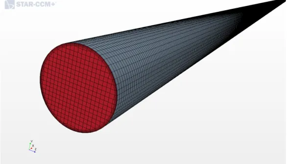
Fluid flow in a straight pipe is the most basic internal flow configuration that is used and has been studied extensively, leading to very well known correlations and results for the friction factor in this flow. Thus, this was the best place to begin learning CFD. A length of 0.5 𝑚 and a diameter of 2 𝑚𝑚 was chosen as this is the geometry to be used in the final model. This geometry had also been simulated by Gezelius along with the semi-circular channels [5]. The mesh for this model can be seen in Figure 3-1.

Figure 3-1: The mesh generated for the simulation of the pressure drop in a straight pipe.

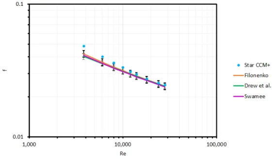
derived by Filonenko, Drew et al., and Swamee-Jain were used as the reference for validation [19][20][21]. The results obtained from Star CCM+ along with the corre-lations and their error bars are plotted in Figure 3-2.

Figure 3-2: Friction factor in a straight pipe over a range of Reynolds number.

Before a Reynolds number of around 8,000, the friction factor values obtained from Star CCM+ do not fall within the error bars of the correlations. This is likely because in this region of Reynolds numbers, the flow may be better modeled by laminar flow or may be in the transition region, in which case the turbulence model would fail to give accurate results. After a Reynolds number of 8,000, the results fall within the error bars of the correlations and follows the same trend, giving confidence to the author for the usage of this model.

3.2.2

Semi-Circular Wavy Channel

The PCHE to be modeled has channels with a semi-circular cross section and a zig-zag configuration. Gezelius modeled the friction factor of a channel with semi-circular cross section and a wavy configuration as shown in Figure 3-3. This configuration was a good reference since it is a channel that has not been studied as extensively as other channels and is similar to that of the semi-circular zig-zag geometry.

Figure 3-3: Geometry of the semi-circular wavy channels with a diameter of 2 and wavelength-to-width ratio of 7.

Two geometries with the diameters, wavelength-to-width ratios and number of wavelengths shown in Table 3.1 were modeled.

Table 3.1: Geometry of the semi-circular wavy channels for pressure drop simulations

Diameter (𝑚𝑚) Wavelength-to-Width Ratio Number of Wavelengths

2 7 12

1.2 30 4

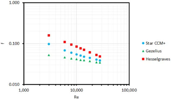
The reference used by Gezelius was a correlation developed by Hesselgraves which was made for the geometry with a diameter of 2 𝑚𝑚 and a wavelength-to-width ratio of 7 [5][22]. The results from Star CCM+ are plotted along with the data obtained by Gezelius and the correlation from Hesselgraves for the first geometry in Figure 3-4. The results from Star CCM+ and from Gezelius for the second geometry are shown in Figure 3-5.

For the first geometry, the results from Star CCM+ can be seen to be in between those of Hesselgraves and Gezelius. This indicates that there may be high uncertainty in the models with this configuration. However, as the Reynolds number increases, the

Figure 3-4: The friction factor in a semi-circular wavy channel with a diameter of 2 mm and wavelength-to-width ratio of 7.

three results seem to converge which presumably means the friction factor is more accurately modeled at higher Reynolds numbers by CFD software. An important consideration for this configuration is that the length from the inlet to the outlet is not the same as that of the total flow length. The data used from Gezelius in these plots used the length from the inlet to outlet while the friction factor computed from Star CCM+ for this configuration used the total fluid flow length which could explain why the data is closer to that of Hesselgraves.

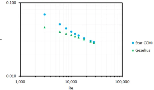
For the second geometry, the friction factor computed from Star CCM+ did not account for the total flow length to allow for a true comparison between the data from Gezelius. Again, the data does not seem to agree for low Reynolds numbers but seems to converge with that of Gezelius as the Reynolds number increases. Similar to Figure 3-4, the data from Star CCM+ is higher than that from Gezelius, indicating that had the data from Gezelius for the first geometry accounted for the total fluid flow, there would still be a disparity between the three studies. While the simulations for the wavy channels did not agree completely with other studies, it was shown that the models followed the general trend and that the differences were likely due to the transition flow and simple turbulence model. The agreement of the study in Section

Figure 3-5: The friction factor in a semi-circular wavy channel with a diameter of 1.2 mm and wavelength-to-width ratio of 30.

3.2.1 along with the general agreement of the wavy channels indicated the author was able to properly model fluid flow through CFD.

3.3

Heat Exchanger Simulations

3.3.1

Configuration of Heat Exchanger

The next component to be verified was the proper integration of heat transfer in the CFD models. This was done by modeling a PCHE from HeatricTM_{which was modeled}

by Van Meter [4]. The design information needed for the model of the PCHE that was modeled was provided by Ishizuka et al. from the Tokyo Institute of Technology (TiTech) and is summarized in table 3.2 [23]. A cross section of the PCHE is shown in figure 3-6.

3.3.2

Model and Conditions

The same models that were used for the friction factor studies in Section 3.2 were used for the fluid flow of this study. To model the heat transfer, the segregated fluid

Table 3.2: Design of the PCHE from TiTech

Primary Side Secondary Side Channel Shape Semi-Circular Semi-Circular

Configuration Straight Straight Diameter (𝑚𝑚) 1.88 1.88 Plate Thickness (𝑚𝑚) 1.63 1.63 Number of Channels 144 66

Length (𝑚𝑚) 896 896

Fluid CO2 Water

Figure 3-6: Cross section of PCHE from TiTech [4]

temperature model was used to specify the inlet temperatures of the fluid at the inlet. Velocity inlets and pressure outlets were used. A trimmer mesh was used for the fluids while a polyhedral mesher was used for the steel plates. The base size used was 0.3 𝑚𝑚 and 2 prism layers with 60% prism layer thickness. Three mass flow rates were tested by Van Meter that recreated the experimental conditions that were conducted which are summarized in Table 3.3.

The two fluids were taken to be at 8 MPa at the inlet. Since the CO2 at these conditions is near the pseudocritical point at 8 MPa, the properties of CO2 had to

be imported to account for the large variations that occur in the thermophysical properties near this point. The density of CO2 and the polynomial fit that was used

Table 3.3: Inlet conditions for TiTech PCHE Simulation

Primary Side Secondary Side Test Pressure (𝑀 𝑃 𝑎) Mass Flow Rate (𝑘𝑔/𝑠) Inlet Temperature (∘𝐶) Mass Flow Rate (𝑘𝑔/𝑠) Inlet Temperature (∘𝐶) 1 8.003 100.53 88.63 701.59 35.63 2 7.972 297.14 89.36 701.80 35.05 3 7.995 500.61 87.93 700.09 31.28

is found in Appendix A along with the other properties that were input into Star CCM+ and taken from NIST [24].

The modeled PCHE was in counterflow configuration with two plates of the hot CO2, each with 12 channels. The cold water plate contained 11 channels. Van meter

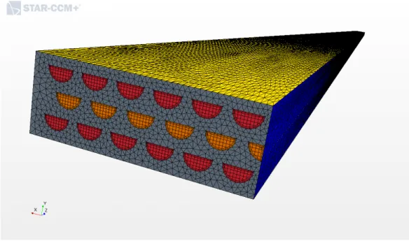
modeled this configuration with CFD by modeling a plate with 5 1/2 cold channels in between two plates with 6 channels each. A symmetry condition was then used on the side which cut halfway through the 6th channel in the cold plate which resulted in the 1/2 channel. This symmetry plane can be see in figure 3-6. A periodic condition was used on the top and bottom face of the configuration and the other side had an adiabatic boundary. This configuration and set of boundary conditions was also used in the Star CCM+ model. The mesh of this configuration can be seen in figure 3-7 with the periodic conditions represented by the yellow surface and the symmetry condition represented by the blue surface.

3.3.3

Results

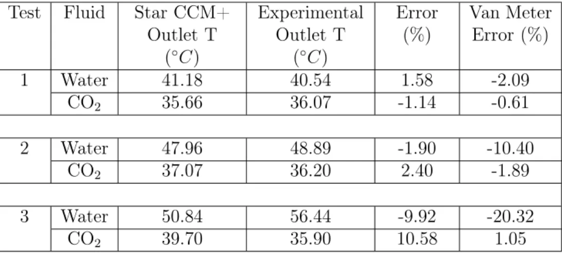
The outlet temperatures served as the basis for comparison between the Star CCM+ model and the experimental results. Surface averages were taken of the outlet tem-peratures of each of the hot channels and then an average was taken among all of them. The same was done for the cold channels. The results from both tests are presented in Table 3.4 along with the error of the Star CCM+ model compared to the experimental results.

Figure 3-7: Mesh of the PCHE from TiTech with CO2 and water

seems to be increasing as the mass flow rate increases (subsequent tests had increasing mass flow rates of the CO2). Even for test 3 with a mass flow rate of 500 𝑘𝑔/𝑠 of CO2,

the error was within Van Meter’s reported error. It should be noted that when the water error was positive, the CO2 error was negative and vice versa which should be

true to maintain an energy balance. While the error from Van Meter for the CO2 was

lower than that from Star CCM+, the error for the water was larger and the errors did not seem to indicate a conservation of energy. Thus, the simulations performed on Star CCM+ seem to show an improvement over those made by Van Meter and were in close agreement to those from the experiment. The results supported by the ability of the author to effectively model PCHE thermal hydraulic performance with CFD.

Table 3.4: Simulated versus experimental outlet temperatures and pressure drops

Test Fluid Star CCM+ Outlet T (∘𝐶) Experimental Outlet T (∘𝐶) Error (%) Van Meter Error (%) 1 Water 41.18 40.54 1.58 -2.09 CO2 35.66 36.07 -1.14 -0.61 2 Water 47.96 48.89 -1.90 -10.40 CO2 37.07 36.20 2.40 -1.89 3 Water 50.84 56.44 -9.92 -20.32 CO2 39.70 35.90 10.58 1.05

Chapter 4

PCHE Steam Generator Modeling

4.1

Introduction

The goal of the project is to evaluate the performance of of a PCHE used as a steam generator in different configurations through the use of CFD software. This would essentially be an extension of the work done by Haratyk et al in which boiling in a straight channel PCHE was simulated through a 1-D MATLAB code. Thus, the configuration that was simulated in such paper served as a natural reference to begin the modeling of the boiling process in a PCHE through CFD.

To model the boiling process, an additional boiling model was needed in addition to those used in section 3.3. The wall boiling model with the Rohsenow correlation discussed in section 2.3 was chosen to model this process within the heat exchanger. The Prandtl number exponent in equation 2.1 is usually taken as either 1 or 1.73 with 1 being typically used for water [3]. The liquid-surface coefficient can generally have a value in the range of 0.0027 to 0.015 depending on the combination of the fluid and the heating surface [25]. In the case of the PCHE from HeatricTM_{, the material}

is chemically etched stainless steel which is combined with water for this project. Jabardo et al. suggested a coefficient of 0.008 and a Prandtl number exponent of 1 for the combination of water and stainless steel [18]. Welty, Wicks, Wilson, and Rorrer recommended a coefficient of 0.0133 for water and chemically etched stainless steel [26]. The range and uncertainty of values used for this correlation required a

study in which multiple values were tested to determine which coefficients should be used when simulating the ultimate models. The best fit coefficients would be determined by bench-marking against the results obtained by Shirvan’s 1-D model which simulated the boiling in a straight configuration PCHE.

4.2

Straight Channel PCHE Boiling

4.2.1

Model and Setup

The geometry of the PCHE that was modeled first is that of a straight channel with semi-circular cross section with a diameter of 2 𝑚𝑚 and a length of 0.5 𝑚. This is the same geometry that was modeled by Shirvan. Channels had a vertical pitch of 1.6 𝑚𝑚 and a horizontal pitch of 2.65 𝑚𝑚. This geometry can be seen in figure 4-1. The inlet conditions that were modeled by Shirvan are summarized in table 4.1.

Figure 4-1: Geometry of the straight channel PCHE steam generator [6]

Table 4.1: Properties of the semi-circular PCHE boiling model [6]

Primary Side Secondary Side Fluid Water Water Number of Channels 147,165 147,165 Inlet Pressure (𝑀 𝑃 𝑎) 15.5 6.0 Mass Flux (𝑘𝑔/𝑚 − 𝑠) 1750 180 Reynolds Number 27,285 1,758 Inlet Temperature (∘𝐶) 325.0 215.6 Outlet Temperature (∘𝐶) 289.8 297.7 Pressure Drop (𝑘𝑃 𝑎) 39 6.6

Since the number of channels is large, one hot and one cold channel could be modeled as being surrounded by infinitely many channels with a periodic condition between the top and bottom and between the left and right walls. Figure 4-2 illus-trates the model being described with the mesh that was generated for the fluids and solid. The two channels were stacked one above the other and were placed within a rectangular piece of stainless steel. On the sides, the thickness of the steel was 0.325 𝑚𝑚 which was half of the horizontal pitch (2.65 𝑚𝑚) minus the diameter of the channel (2 𝑚𝑚). Above the hot channel and below the cold channel, the thickness was 0.3 𝑚𝑚 which was half of the vertical pitch (1.6 𝑚𝑚) minus the diameter (1 𝑚𝑚). This ensured the periodic conditions accurately replicated the arrangement of all the channels in the PCHE. The mesh that was used was stretched by a factor of 4 in the direction of the flow to minimize the size of the mesh and the time required for computation. The total number of cells used for these simulations was 1,319,434. The stopping criteria used was a standard deviation for the surface average outlet temperatures of both channels as well as for the pressure drops. For the pressure drops, a standard deviation of 50 𝑃 𝑎 over 20 steps was used and for the outlet tem-peratures, a standard deviation of 0.5 ∘𝐶. The same stopping criteria is used for all subsequent simulations. All outlet temperatures evaluated are surface averaged temperatures over the outlet.

4.2.2

Determining Coefficients for the Rohsenow Correlation

Using the coefficients recommended in section 4.1, a range of liquid-surface coefficients and Prandtl number exponents were tested. The outlet temperatures and pressure drops in the hot and cold channels were evaluated to be compared to the results from the 1-D code. While this is a good benchmark to use in order to find the proper coefficients for the model, those results were used as a loose comparison since the 1-D model would not be as accurate as the 3-D model used by Star CCM+.

Table 4.2 shows the values that were tested for the liquid-surface coefficient and the Prandtl number exponents along with the outlet temperatures and pressure drops for the hot and cold channels. From the data, it can be seen that as the coefficient

Figure 4-2: Mesh of the single set of channels in straight PCHE

𝐶𝑞𝑤 increases, the secondary side outlet temperature decreases. In contrast, when the

Prandtl number exponent increases, the secondary side outlet temperature increases. The primary side outlet temperature has almost negligible changes with the coefficient and Prandtl number exponent. This makes sense because the boiling correlation describes the amount of heat that flows into the boiling fluid from the wall which would have a large effect on the boiling water and not a large effect on the primary side fluid.

Similar to the temperatures, the pressure drop in the primary side had minimal change due to the change in the coefficients. This is expected since the coefficients affect the boiling of the secondary side. The pressure drop is thus only coupled to the coefficients through the change in properties of the primary side as it increases or decreases in temperature. The variation in outlet temperatures of the primary side is about 1 ∘𝐶 which would not be enough to change the properties enough for large variations in pressure drop. In the secondary side, however, there is a much larger variation in the pressure drop since it is highly dependent on the boiling process. Liquid water will contribute more to the pressure drop due to its higher density so the longer the secondary side fluid stays liquid, the higher the pressure drop will

Table 4.2: Outlet temperatures and pressure drops for varying coefficients in the Rohsenow correlation

Primary Side Secondary Side 𝐶𝑞𝑤 𝑛 Outlet Temperature (∘𝐶) Pressure Drop (𝑘𝑃 𝑎) Outlet Temperature (∘𝐶) Pressure Drop (𝑘𝑃 𝑎) 0.0027 1 288.7 20.28 305.3 4.21 0.01 1 289.1 20.36 301.3 3.96 0.013 1 289.2 20.14 299.5 3.86 0.0133 1 289.2 20.22 299.3 3.85 0.015 1 289.2 20.23 298.1 3.76 0.02 1 289.7 20.29 295.0 3.67 0.08 1 292.4 20.23 278.5 3.06 0.01 1.73 288.9 20.21 301.9 3.97 0.0133 1.73 289.1 20.16 300.1 3.86 0.02 1.73 289.4 20.20 296.3 3.69

become. The length required for water to travel before boiling is directly dependent on the boiling correlation and thus the coefficients.

While the pressure drop in the secondary side had relatively large variations with most of them being much lower than that of the 1-D model, this was not a huge concern as the correlations for the pressure drop of two-phase flow in a semi-circular channel are extremely limited. Thus, the pressure drop of the secondary fluid from the 1-D model could not be used as an accurate benchmark. On the other hand, the much lower pressure drop in the primary side from Star CCM+ compared to the 1-D model was a cause for concern since the correlations for single-phase flow have are much more reliable. This required a hand calculation to validate the pressure drop. The pressure drop in a straight channel can be roughly approximated by that for a straight pipe by replacing the hydraulic diameter. The pressure drop equation is

∆𝑃 = 𝑓2𝜌𝐿𝑣

2

2𝐷𝐻

(4.1)

where 𝑓 is the friction factor which can be obtained from the Moody chart for pipes which will result in an error of around ±15% [27]. The stainless steel was assumed

to be smooth to obtain a friction factor of around 𝑓 = 0.027. Using the semi-circle geometry and the inlet properties, a pressure drop of around 25.38 𝑘𝑃 𝑎 was obtained. This result is much closer to the approximately 20 𝑘𝑃 𝑎 that was obtained from Star CCM+ than the 39 𝑘𝑃 𝑎 which was obtained from the 1-D model. The difference in pressure drop could potentially be explained if the 1-D model included the pressure drop from headers.

One of the tests that were studied used coefficients that were outside of the range of the recommended values to determine how it would affect the results. This value of 𝐶𝑞𝑤 = 0.08 gave a secondary outlet temperature of 278.5∘𝐶 which is about 16∘𝐶

lower than any of the other results. This shows that using values outside of the range could drastically affect the results if values outside the range are used instead.

Determining the appropriate coefficients to use in the final studies required a bal-ance between keeping the outputs reasonably close to those from the 1-D model while also considering the validity of that model. Additionally, values that are considered to be reasonable for these coefficients should be chosen. As mentioned earlier, a liquid-interface coefficient of 𝐶𝑞𝑤 = 0.0133 was recommended for chemically etched stainless

steel and water and the Prandtl exponent number of 1 was recommended for water. This combination proved to give the closest outlet temperatures to those of 1-D model for both the primary and secondary fluids. Testing multiple coefficients gives a good idea on the sensitivity: with the value of 𝐶𝑞𝑤 = 0.013 and 𝑛 = 1, a secondary side

outlet temperature of 299.5∘𝐶 compared to the 299.3∘𝐶 obtained from 𝐶𝑞𝑤 = 0.0133

and 𝑛 = 1. This difference in outlet temperature is small but is important to note. Similarly, if 𝐶𝑞𝑤 = 0.0133 is used and the Prandtl number exponent is changed to

𝑛 = 1.73, the secondary side outlet temperature increases by about 3∘𝐶 to 300.1∘𝐶. Again, this is not a large change in temperature but can still lead to some errors.

After analyzing the results obtained from the different coefficients, the combina-tion of 𝐶𝑞𝑤 = 0.0133 and 𝑛 = 1 were chosen. These values were chosen due to their

nearly equal results from the 1-D model and having been recommended by Welty et al.

4.2.3

Sensitivity Study

When modeling the boiling in these channels in a zig-zag configuration, the mesh could not be scaled in the direction of the flow due to its shape. This would make a finer mesh which would result in larger computational times. Additionally, when modeling the boiling with one channel plugged, a grid of channels was modeled in order to change one of them from having flowing water in the channel to still air. This resulted in a computation that was too large to run, requiring a coarser mesh. Thus, a sensitivity study was done on the straight channel configuration to ensure that the results would not change drastically if a coarser mesh was used for the zig-zag.

Table 4.3: Comparison of meshes used in straight channel boiling

Fluid Mesh Solid Mesh Base Size

(𝑚𝑚)

Number of Prism Layers

Base Size Mesh Scale

Cells Mesh 1 0.15 4 0.15 0.25 1,319,434 Mesh 2 0.15 4 1 1 1,875,795

Since the boiling interaction is extremely important and requires a fine mesh, the fluid mesh was not changed besides the scaling which was no longer used. Thus, only the mesh for the solid body was modified to reduce the size of the file. The differences in the meshes are shown in table 4.3 where mesh 1 is the mesh that was used for all previous cases and mesh 2 is the mesh that was studied and used for the zig-zag configuration with multiple channels modeled. The mesh scale again refers to the scaling factor used in the direction of the flow of the fluid. For this study, the values of 𝐶𝑞𝑤 = 0.0133 and 𝑛 = 1 were used as these were the values chosen to be

used for subsequent models.

The results for the sensitivity study are shown in table 4.4 which compare the outlet temperatures for the two meshes. The only significant difference worth looking at is that of the secondary side outlet temperature since all other outputs are nearly identical. Even for the secondary side outlet temperature, the difference is only 1.87∘ which is not a large deviation. However, it is still important to keep this in mind as

Figure 4-3: Mesh 2 of the single set of channels in straight PCHE

this difference could be larger when other conditions are introduced such as the one plugged channel.

Table 4.4: Outlet temperatures and pressure drops for mesh sensitivity study

Primary Side Secondary Side Mesh Outlet Temperature (∘𝐶) Pressure Drop (𝑘𝑃 𝑎) Outlet Temperature (∘𝐶) Pressure Drop (𝑘𝑃 𝑎) Mesh 1 289.2 20.22 299.3 3.85 Mesh 2 289.0 20.25 298.9 3.85

After running a mesh sensitivity study, a turbulence model sensitivity study was also performed to ensure the results would be reasonably similar with other models. A standard k-epsilon, two-layer all y+ wall turbulence model was simulated as well. The total cells used in the model were 1,939,947. The results from this study are presented in table 4.5

The main difference in results between the two models is that of the primary side pressure drop and the secondary side outlet temperature. The pressure drop in-creased while the outlet temperature dein-creased from the realizable model used

previ-Table 4.5: Comparison of results from different turbulence models

Primary Side Secondary Side Model Outlet Temperature (∘𝐶) Pressure Drop (𝑘𝑃 𝑎) Outlet Temperature (∘𝐶) Pressure Drop (𝑘𝑃 𝑎) Realizable k-epsilon

Two-Layer All y+ Wall 289.2 20.22 299.3 3.85 Standard k-epsilon

Two-Layer All y+ Wall 289.5 21.76 296.9 4.00

ously. However, the differences are still within the error expected from using different turbulence models. The pressure drops and outlet temperatures are all still within the expected range of values and are still reasonably close to the results from the 1-D model. Thus, it is shown that the results are not very sensitive to different turbulence models and meshes, suggesting that the models used give reasonable results.

4.2.4

Orientation of PCHE With Respect to Gravity

One design choice that was not considered by Haratyk et al. was that of the orien-tation of the PCHE with respect to gravity. If the PCHE was setup vertically such that gravity is aligned with the flow of the hot channel, there could be certain im-provements to the performance such as a lower pressure drop over the channel. A quick simulation was run to compare the results from the previous configuration in which gravity was perpendicular to the flows to the vertical layout. The results are compared in table 4.6 in which horizontal refers to the previous layout and vertical refers to the layout with gravity aligned with the primary side flow.

While there was not much change in the outlet temperatures of the two channels, there is a significant change in the pressure drops across the channel. The pressure drop in the primary side is decreased by almost 4 𝑘𝑃 𝑎 whereas the pressure drop of the secondary side is increased by only 1.2 𝑘𝑃 𝑎.

An interesting aspect of boiling to look at is the flow of two-phase fluid through the channel to visualize where the steam and liquid concentrates. Figure 4-4 shows a plane

Table 4.6: Outlet temperatures and pressure drops in different orientations

Primary Side Secondary Side Layout Outlet Temperature (∘𝐶) Pressure Drop (𝑘𝑃 𝑎) Outlet Temperature (∘𝐶) Pressure Drop (𝑘𝑃 𝑎) Horizontal 289.2 20.22 299.3 3.85 Vertical 289.3 16.61 298.2 5.06

that cuts through the center of the channel in both the (a) horizontal configuration and (b) vertical configuration. The models in this figure have been scaled by a factor of 1/10 to make it easier to visualize. In the horizontal configuration, the liquid that has not boiled off at the beginning which is represented by the blue stream concentrates at the bottom of the channel since the gravity points in the negative y direction. In the vertical configuration, the liquid is more symmetrically distributed through the channel. This may be preferable to keep any particles within the fluid away from the walls to prevent buildup.

4.3

Zig-Zag Channel PCHE Boiling

4.3.1

Model and Setup

The final goal of the project was to extend the boiling study in a PCHE to the zig-zag geometry to evaluate the enhancement of the performance compared to the straight channel. The geometry of zig-zag configuration is shown in figure 4-5. The idea behind the zig-zag shape is that it will enhance the heat transfer in the channel which results in better performance as a heat exchanger.

A single channel was modeled with periodic conditions between the top and bot-tom and between the left and right walls similar to that of the straight channel. To have a fair comparison between between the two configurations, the same configura-tion used for the straight channel was used. This meant that the actual flow length should be made equal to that of the straight channel which was 0.5 𝑚. An integer

(a)

(b)

Figure 4-4: Vapor fraction in the y-z plane of the channel of boiling water in a (a) horizontal configuration and (b) vertical configuration

number of the "zigs" had to be used to keep the inlets the same between the primary and secondary side. A total of 64 "zigs" were used for a total flow length of 0.498 𝑚. This small difference in the total fluid length was assumed to have a negligible effect on the performance so that the two geometries could be compared. Additionally, the thickness of the steel surrounding the channels were kept the same throughout the entire channel. Figure 4-6 shows this configuration with the mesh used. The mesh

Figure 4-5: Geometry of the zig-zag channel

used is the same as mesh 2 described in section 4.2.3. The same realizable k-epsilon, two-layer all y+ wall turbulence model was used as in the other simulations.

Figure 4-6: Mesh of the single zig-zag channel

4.3.2

Boiling Results With Single Channel Periodicity

The results from the zig-zag boiling simulation are shown in table 4.7 along with those from the straight configuration for comparison. Immediately it can be seen that the outlet temperature of the secondary side is much higher than that of the straight channel PCHE. The outlet temperature corresponds to a super heat of around 45∘𝐶 compared to the super heat of around 22 ∘𝐶 of the straight channel. This is highly desirable as it can lead to a higher thermal efficiency of the power cycle.

A major disadvantage of using a zig-zag PCHE compared to a straight PCHE is that the pressure drop increases significantly due to the increased disturbances to

Table 4.7: Comparison of outlet temperatures and pressure drops from boiling in a straight and zig-zag PCHE

Primary Side Secondary Side Outlet Temperature (∘𝐶) Pressure Drop (𝑘𝑃 𝑎) Outlet Temperature (∘𝐶) Pressure Drop (𝑘𝑃 𝑎) Straight 289.9 20.22 297.0 3.86 Zig-Zag 286.2 92.52 319.7 15.74

the flow. The primary side pressure drop is nearly 4.5 times greater than that of the straight PCHE while the secondary side has a pressure drop slightly more than 4 times greater. This will lead to higher pumping power required to drive the flow of the fluid. This increased pumping power could even offset any increase in power from the increased outlet temperature of the secondary side. Calculations would need to be performed to determine whether the advantages from the zig-zag configuration offset the disadvantages, though calculated pressure drops are of reasonable range.

Figure 4-7: Volume fraction of vapor in the secondary side in the zig-zag PCHE

PCHE as a steam generator is the possibility of plugging. To see how this could affect the performance, it is important to see the flow path of the fluid and two-phase mixture. Figure 4-7 shows the volume fraction of vapor in the secondary side in the region where boiling begins to occur. A streamline with colors representing lower volume fraction of vapor can be seen flowing near the center of the channel. This is the most favorable path of the fluid as it travels through the zig-zag configuration, especially for the fluid with smaller volume fractions of vapor. If debris were to accumulate near the sharp inner corners, this could greatly obstruct the flow of the fluid and lead to problems in the boiling process. On the other hand, were debris to accumulate near the outer sharp corners, a smaller effect on the flow would likely be result. This should be an important consideration for the future design of the PCHE.

Figure 4-8: Surface average temperature along the z-direction of the heat exchanger of the two fluids

Figure 4-8 shows the surface average temperatures of the two fluids along the z-direction. The total length of the heat exchanger and thus the length the fluid travels in the z-direction is 448 𝑚𝑚. The primary side inlet is at z = 0 𝑚𝑚 and the

secondary side inlet is at z = 448 𝑚𝑚. By superheating the steam in the secondary side, the pinch point which otherwise would have occurred at the location of the onset of boiling in the secondary side instead occurs at the outlet. This pinch point is much lower at around 5∘𝐶.

The overall heat transfer coefficient of the heat exchanger can be derived by using the logarithmic mean temperature difference method. To do so, the heat exchanger is divided into three sections based on the secondary fluid: 1) the subcooled region 2) the saturated region and 3) the superheated region. The heat flow rate is obtained in each of the sections using the equation

𝑄 = ˙𝑚𝑐𝑝∆𝑇 (4.2)

where the specific heat 𝑐𝑝 can be averaged over the temperature range. The primary

side would be used for this equation since in the section of saturated water in the secondary side, ∆𝑇 = 0. This heat flow rate would then be equated to that obtained in each section from the equation using the LMTD. This equation is

𝑄 = 𝑈 × 𝐴 × 𝐿𝑀 𝑇 𝐷 (4.3)

where 𝑈 is the overall heat transfer coefficient, 𝐴 is the heat flow area and the 𝐿𝑀 𝑇 𝐷 is defined as

𝐿𝑀 𝑇 𝐷 = (𝑇𝑝,𝑖− 𝑇𝑠,𝑜) − (𝑇𝑝,𝑜− 𝑇𝑠,𝑖) 𝑙𝑛(𝑇𝑝,𝑖− 𝑇𝑠,𝑜) − 𝑙𝑛(𝑇𝑝,𝑜− 𝑇𝑠,𝑖)

(4.4)

where 𝑇𝑝,𝑖 is the primary side inlet temperature, 𝑇𝑝,𝑜 is the primary side outlet

tem-perature, 𝑇𝑠,𝑖 is the secondary side inlet temperature and 𝑇𝑠,𝑜 is the secondary side

outlet temperature. The heat transfer coefficients times the heat transfer areas are presented in table 4.8 for both the zig-zag PCHE and the straight PCHE for compar-ison.

The heat transfer coefficient is largest in the saturated region and lowest in the superheated region for both configurations. This was expected since boiling is an effective method to transfer heat and should thus have a large heat transfer coefficient.

Table 4.8: Heat transfer coefficients times the heat transfer area of the different regions in the PCHE

U (𝑊/𝑚−2· 𝐾) Region Straight Zig-Zag Subcooled Liquid 4934.3 6627.2

Saturated 8420.1 12096.6 Superheated Vapor 3127.2 5260.4

Likewise, the superheated vapor region would have a lower heat transfer coefficient due to its lower thermal conductivity and other properties that lend it to be a poor choice for transferring heat. According to Mills, typical overall heat transfer coefficients for water to water heat exchangers is on the order of 800-2500 while that of water to gas is around 10-50 and that of steam boilers is about 10-40 [16]. The overall heat transfer coefficients obtained here are much larger than these typical heat transfer coefficients and thus shows great performance of the PCHE. It is also noted that the heat transfer coefficients are larger for the zig-zag configuration for the three regions by factors of around 1.3, 1.4 and 1.7 respectively. Thus, it is clear that the zig-zag configuration provides better heat transfer from the primary side to the secondary side compared to the straight PCHE.

4.3.3

Changing Orientation of Gravity

Similar to the case of the straight channel in section 4.2.4, a study was done to deter-mine the effect of changing the orientation of the PCHE from horizontal to vertical. Again, the vertical orientation had the primary side fluid flowing in the direction of gravity to take advantage of natural circulation. The model is the same as that used in the horizontal orientation. The results from the simulation are summarized in 4.9. There is a negligible difference in the outlet temperatures of the two orientations. The difference in pressure drop when the zig-zag PCHE is used in the vertical ori-entation compared to the horizontal configuration is smaller than that of a straight PCHE. The primary side pressure drop is only about 3.3 𝑘𝑃 𝑎 less which is small

Table 4.9: Outlet temperatures and pressure drops from boiling in a vertical PCHE

Primary Side Secondary Side Outlet Temperature (∘𝐶) Pressure Drop (𝑘𝑃 𝑎) Outlet Temperature (∘𝐶) Pressure Drop (𝑘𝑃 𝑎) 286.0 89.23 319.6 16.38

relative to the total pressure drop. A similar situation occurs on the secondary side with only about 0.7 𝑘𝑃 𝑎 increase. If a zig-zag PCHE is used, which is the standard design from HeatricTM, the orientation of the PCHE would not have a large affect on the pressure drop and pumping power required. Thus, if there are other more important aspects to consider when determining the orientation, the pressure drop should not be a large concern.

4.3.4

Plugging of a Single Channel in Secondary Side

The small size of the channels in a PCHE makes it likely to have blockage that would plug a channel due to the debris that could be present in the water. Boiling the water could increase the likelihood of this plugging phenomenon to occur. Since there is a large amount of channels in the PCHEs, a relatively large number of plugged channels can be tolerated before a reduction in performance is seen. However, if channels are plugged, problems could arise within the channels surrounding the plugged channels. Specifically, if a secondary side channel is plugged and is filled with still air instead of the flowing water, local hot spots can occur. This phenomenon is important to study to ensure the integrity of the PCHE is not compromised and to determine the effect on neighboring channels. Studying the effect of a single plugged channel on the performance can also be used to determine how many plugged channels can be tolerated before a significant change in the performance occurs.

To model plugging of a single channel, 2 sets of the vertically stacked primary and secondary side plates were modeled with 3 channels horizontally. A single secondary side channel in the middle of a singe plate was filled with still air instead of flowing

Figure 4-9: Model of multiple channels with a single channel in the secondary side filled with air

water throughout the entire channel. Periodicity conditions were set between the top and bottom and between the left and right and it was assumed that the disturbances created by the periodic air channels were negligible to those channels surrounding it. A diagram of the model with the mesh used and labels for each of the channels is shown in figure 4-9. The mesh used had a total of 10,592,197 cells and the simulation used a stopping criteria of a standard deviation of 0.1∘𝐶 and 10 𝑃 𝑎 over 20 steps for the outlet temperatures and pressure drops respectively.

The outlet temperatures and pressure drops of all the channels besides the plugged are summarized in table 4.10 while certain values from the plugged channel are pre-sented in table 4.11. It can be seen that in the channels surrounding the plugged channel, the outlet temperatures are higher than without a plugged channel. This is expected since there is one channel less to remove heat from the hot channels above and below it. The hot channels above and below the plugged channel are around 3-4 ∘𝐶 higher than the other hot channels. The cold channels next to the plugged channel are less than 1 ∘𝐶 higher than the rest of the cold channels. This indicates that the main effect of the plugged channel is on the hot channels directly above and

Table 4.10: Outlet temperatures and pressure drops in the channels surrounding the plugged channel

Channel Outlet Temperature (∘𝐶) Pressure Drop Cold 1 323.6 16.57 Cold 2 323.7 17.54 Cold 3 323.5 16.86 Cold 4 324.0 17.88 Cold 6 323.9 17.94 Hot 1 287.4 95.04 Hot 2 291.2 95.37 Hot 3 287.5 95.32 Hot 4 287.1 95.44 Hot 5 290.7 95.44 Hot 6 287.1 95.53

below it. It is interesting to note that the pressure drops and outlet temperatures are higher in all of the channels than was obtained from the single channel model. This may indicate that the other plugged channels that are being modeled as a result of the periodic boundary conditions may have a non-negligible effect on the channels in the mode. A larger set of channels would need to be modeled to verify this, though this computation would require more resources.

Table 4.11: Temperatures in the plugged channel

Temperature at z = 0 (∘𝐶) Temperature at z = 448 (∘𝐶) Max Temperature (∘𝐶) 279.1 324.92 324.96

Chapter 5

Conclusion

The aim of this work was to study the design and performance of a compact steam generator using CFD for the purpose of using it in a nuclear power plant. By using a 1-D MATLAB code which simulated the boiling process of water on the secondary side of a semi-circular, straight channel PCHE, the coefficients of the Rohsenow corre-lation used to model boiling were determined. Specifically, a liquid-surface coefficient of 𝐶𝑞𝑤 = 0.0133 and a Prandtl number exponent of 𝑛 = 1 was chosen for the

cor-relation as they gave good agreement and were recommended for the configuration by previous studies. The agreement obtained between the 1-D MATLAB code and the simulations ran using the CFD program Star CCM+ were within 2 ∘𝐶 for both outlet temperatures, well within the errors expected between a 1-D code and a 3-D simulation.

Once the models used were properly setup, the configuration of the PCHE was extended to the more common design of a zig-zag PCHE from HeatricTM_{. Comparing}

the results of the two designs, there is a notable improvement in the heat transfer capabilities arising from the zig-zag shape. While the straight channel design led to around 22 ∘𝐶 of superheat, the zig-zag channels led to a superheat of around 44

∘_{𝐶. On the other hand, there is a significant increase in the pressure drop across}

the two sides of the heat exchanger. The primary side pressure drop increased from around 20 𝑘𝑃 𝑎 up to around 92 𝑘𝑃 𝑎 and likewise the secondary side pressure drop increased from around 4 𝑘𝑃 𝑎 to around 15 𝑘𝑃 𝑎. The increase in superheat which can