Bayesian Policy Search with Policy Priors

Bayesian Policy Search with Policy Priors

The MIT Faculty has made this article openly available.

Please share

how this access benefits you. Your story matters.

Citation

Wingate, David, Noah D. Goodman, Daniel M. Roy, Leslie P.

Kaelbling, and Joshua B. Tenenbaum. "Bayesian Policy Search with

Policy Priors." Proceedings of the Twenty-Second International Joint

Conference on Artificial Intelligence, July 16-22, 2011, Barcelona,

Spain.

As Published

http://dx.doi.org/10.5591/978-1-57735-516-8/IJCAI11-263

Publisher

International Joint Conference on Artificial Intelligence (IJCAI)

Version

Author's final manuscript

Citable link

http://hdl.handle.net/1721.1/87054

Terms of Use

Creative Commons Attribution-Noncommercial-Share Alike

Bayesian Policy Search with Policy Priors

David Wingate

, Noah D. Goodman

, Daniel M. Roy

, Leslie P. Kaelbling

and Joshua B. Tenenbaum

1

_{BCS / CSAIL}

Massachusetts Institute of Technology

{

wingated,droy,lpk,jbt

}

@mit.edu

2

_{Department of Psychology}

Stanford University

ngoodman@stanford.edu

Abstract

We consider the problem of learning to act in partially observable, continuous-state-and-action worlds where we have abstract prior knowledge about the structure of the optimal policy in the form of a distribution over policies. Using ideas from planning-as-inference reductions and Bayesian un-supervised learning, we cast Markov Chain Monte Carlo as a stochastic, hill-climbing policy search al-gorithm. Importantly, this algorithm’s search bias is directly tied to the prior and its MCMC pro-posal kernels, which means we can draw on the full Bayesian toolbox to express the search bias, includ-ing nonparametric priors and structured, recursive processes like grammars over action sequences. Furthermore, we can reason about uncertainty in

the search bias itself by constructing a

hierarchi-cal prior and reasoning about latent variables that determine the abstract structure of the policy. This yields an adaptive search algorithm—our algorithm

learns to learn a structured policy efficiently. We

show how inference over the latent variables in these policy priors enables intra- and intertask transfer of abstract knowledge. We demonstrate the flexibility of this approach by learning meta search biases, by constructing a nonparametric finite state controller to model memory, by discovering motor primitives using a simple grammar over primitive actions, and by combining all three.

1

Introduction

We consider the problem of learning to act in partially ob-servable, continuous-state-and-action worlds where we have abstract prior knowledge about the structure of the optimal policy. We take as our running example domain a mobile robot attempting to navigate a maze. Here, we may have sig-nificant prior knowledge about the form of the optimal policy: we might believe, for example, that there are motor primitives (but we don’t know how many, or what sequence of actions each should be composed of) and these primitives can be used by some sort of state controller to navigate the maze (but we don’t know how many states it has, or what the state

transi-tions look like). How can we leverage this knowledge to aid us in searching for a good control policy?

The representation of abstract, vague prior knowledge for learning has been studied extensively, and usefully, within the literature on hierarchical Bayesian models. Using hierarchi-cal Bayesian models, we can express prior knowledge that, e.g., there are reusable components, salient features, etc., as well as other types of structured beliefs about the form of op-timal policies in complex worlds. In this work, we use non-parametric priors whose inductive biases capture the intuition that options, states and state transitions useful in the past are likely to be useful in the future. The use of nonparametric distributions also allows us to infer the relevant dimensions both of motor primitives and state controllers.

We can take advantage of the abstract knowledge encoded in the policy prior by recasting the policy optimization prob-lem as an inference probprob-lem through a transformation loosely related to planning-as-inference reductions [Toussaint et al., 2006; Botvinick and An, 2008]. By combining this reduction with a policy prior, probabilistic inference finds good policies by simultaneously considering the value of individual policies and the abstract knowledge about the likely form of optimal policies encoded in the policy prior.

In particular, if we use MCMC to perform inference, then we can interpret the resulting algorithm as performing a type of stochastic search. Importantly, the way MCMC traverses the policy space is tied to the prior and its proposal kernels. If we use a hierarchical prior, and reason about the prior over priors at the same time as the policy, then we are effectively reasoning about the uncertainty in the search bias itself. The prior allows us to apply what we learn about the policy in one region to the search in other regions, making the overall search more efficient—the algorithm learns to learn struc-tured policies. To see this, consider a simple maze. If expe-rience suggests that going north is a good strategy, and if the idea of a dominant direction is captured as part of a hierar-chical policy prior, then when we encounter a new state, the policy search algorithm will naturally try north first. In simple domains, the use of abstract knowledge results in faster learn-ing. In more complex domains, the identification of reusable structure is absolutely essential to finding good policies.

We explain our setup in Section 2, define our algorithm in Section 3, and show examples of the kinds of policy priors we use in Section 4. We conclude in Section 5.

2

Background and Related Work

Each environment we consider can be modeled as a standard (PO)MDP. LetM be a POMDP with state space S, actions A, observations O, reward function R : S → R.

In the first experiment, we assume the state is fully-observable and so a policy π is a mapping from states to dis-tributions over actions. In the latter two experiments, the state is partially-observable and we restrict our policy search to the space of finite state controllers whose internal state transitions depend on the current internal state and external observation generated by the world. In both cases, the value V(π) of a policy π ∈ Π in the space of policies Π under consideration is defined to be the expectation of the total reward received while executing the policy:

V(π) = Eπ "_t=∞ X t=0 rt #

In this work, we assume we can evaluate the value V(π) of each policy π; in practice we approximate the value using roll-out to form a Monte Carlo estimator. We refer the reader to [Kaelbling et al., 1998] for more details on the (PO)MDP setting.

We use the policy estimation function V(π) to guide a pol-icy search. In model-based reinforcement learning, polpol-icy search methods (such as policy iteration [Howard, 1960] or policy gradient [Williams, 1992]) explicitly search for an op-timal policy within some hypothesis space.

A central problem in model-based policy search methods is guiding the search process. If gradient information is avail-able, it can be used, but for structured policy classes involving many discrete choices, gradient information is typically un-available, and a more general search bias must be used. This search bias usually takes the form of a heuristic which is typ-ically fixed, or a cost-to-go estimate based on value function approximation; while not a policy search algorithm, recent success in the game of Go is a striking example of the power of properly guided forward search [Gelly and Silver, 2008].

Recent work by [Lazaric et al., 2007] presents an actor-critic method that bears some resemblance to our approach. They use a particle filter to represent a stochastic policy (we consider a distribution over policies, each of which may be stochastic), and search with sequential Monte-Carlo methods. The focus of the work is learning policies with continuous actions, as opposed to structured actions; in addition, there is no notion of reasoning about the search process itself.

[Toussaint et al., 2008] describe a method for learning the structure of a hierarchical finite state POMDP controller of fixed depth using maximum likelihood techniques. They transform the planning problem into a DBN that exposes the conditional independence structure if the POMDP is factored. In contrast, we make the stronger assumption that we can evaluate the policy value (although in practice we estimate it from several roll outs). Toussaint et al. give complexity bounds for the inner loop of an EM algorithm in terms of the size of the state, action and observation spaces. In contrast, we explore policy search with policy priors in the continuous state space and action space. However, both methods are

us-ing a local search (coordinate-wise ascent and stochastic hill climbing, respectively) to search the space of policies.

3

A Bayesian Policy Search Algorithm

In this section we describe the reduction of policy optimiza-tion to approximate sampling. We begin by describing a sim-ple graphical model in which maximum likelihood (ML) es-timation is equivalent to policy optimization, and then incor-porate our policy prior by considering maximum a posteri-ori (MAP) estimation of the policy parameters. Inference in this model is our policy search algorithm. Given the compo-sitional nature of MCMC algorithms and the wide range of probabilistic models for which we have MCMC algorithms, we can easily construct a variety of policy priors by combin-ing smaller models into complex, structured distributions.

Let V(π) be the value of a policy π ∈ Π, where Π is the space of policies we are considering. We assume that we can evaluate V and that our goal is to find the optimal policy π∗

satisfying π∗= arg max π∈ΠV(π) (1) or, equivalently, π∗= arg max π∈ΠΛ(π),

where Λ(π) = exp{V (π)}. Following [Toussaint et al., 2006; Botvinick and An, 2008], we re-express the optimiza-tion as probabilistic inference, but take a sampling perspec-tive. We begin by introducing an auxiliary binary random variable R whose conditional distribution given the policy π is

p(R = 1|π) = Z−1Λ(π) = Z−1exp{V (π)},

where Z = R

π∈ΠΛ(π)dπ. One can easily verify that the

maximum likelihood policy is π∗_{. In contrast with typical}

reductions of planning to inference, we now introduce a prior distribution p(π) > 0 and consider the posterior distribution

Q(π) ≡ p(π|R = 1) ∝ p(π) Λ(π). (2)

Note that with a uniform prior, the MAP policy is also π∗. Eq. 2 defines our graphical model. Our policy search algo-rithm is to perform MCMC based inference in this model. The resulting Monte Carlo simulation is a local search al-gorithm, which performs a stochastic hill-climbing search through policy space. As with any MCMC method, the search is parameterized by proposal kernels, which depend on the state of the policy and the state of any auxiliary variables, and which will be biased by the policy prior. At the end, the highest value policy is extracted from the sequence.

The policy prior approach is arbitrarily flexible, which has important consequences. In particular, if there are parameters which govern part of the policy prior—e.g., we have an agent who takes steps with an a priori Gaussian stepsize parameter-ized by its mean—we can easily construct a hierarchical prior which places a distribution over those parameters with its own hyperparameters. In general, the prior distribution will be a marginal of a joint distribution p(π, θ) over the policy and latent variables used in the specification of the hierarchical Bayesian model. The MCMC kernels make proposals to both

Algorithm 1 Policy Search with Policy Priors

1: Input: a prior p(π) =R

Θp(π, θ)dθ, policy value

func-tion V, Markov kernels Kπ andKθ, and stopping time

(or condition) T

2: Variables: policy π and auxiliary variables θ.

3: Initialize:(π0, θ0) ∼ p(π, θ).

4: for t= 1, 2, . . . , T do

5: Randomly choose to...

6: propose a new policy: πt+1∼ Kπ(πt, θt)

7: propose a new latent representation: θt+1 ∼

Kθ(πt, θt)

8: If the policy πt+1 changes, recompute V(πt+1) ∝

log p(R = 1|πt+1) (policy evaluation).

9: Accept or reject according to the standard Metropolis-Hastings rule.

10: end for

the policy π as well as the auxiliary variables θ. The process of inferring these latent variables in the policy prior gives us the effect of learning to learn, as we shall see.

The final policy search algorithm is outlined as Alg. 1. In the case of a non-uniform policy prior, the policy which achieves the optimum of Eq. 1 will not in general be equal to the policy which achieves the optimum of Eq. 2 because of the regularizing effect of the prior. For most models, this is not a problem, but can be mitigated if desired by tempering away the prior using a replica exchange algorithm.

4

Experiments

We now present three experiments involving increasingly structured, hierarchical policy priors.

4.1

Compound Dirichlet Multinomial Priors

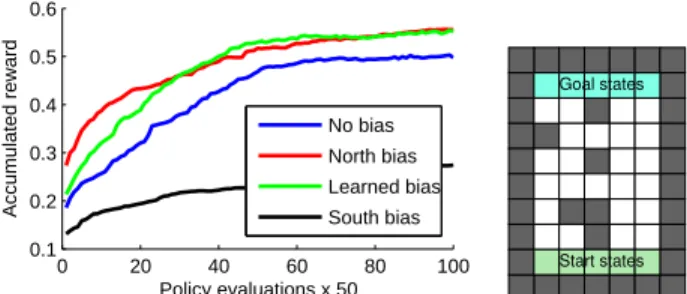
Our first experiment illustrates how a simple hierarchical pol-icy prior can guide the search for an optimal polpol-icy. Consider the maze in Fig. 1. A simple policy prior is generated by randomly sampling actions for each state:

p(π|θ) = Y s∈S p(πs|θ) = Y s∈S Multinomial(θ) (3)

whereMultinomial(θ) is a multinomial distribution over ac-tions. This policy prior states that each state’s action is chosen independently, but all are chosen in a biased way depending on θ. Figure 1, blue line (“No bias”) shows the performance of our algorithm using this policy prior with a uniform θ.

What if θ is not uniform? If θ favors moving north, for example, then the local proposal kernels will tend to propose policies with more north moves first. Figure 1, red line, shows the performance improvement resulting from using such a θ. Encoding the wrong bias – say, favoring southward moves – is disastrous, as shown in Fig. 1, black line.

Clearly, the right bias helps and the wrong bias hurts. What if we don’t know the bias? We can learn the bias at the same time as the optimal policy by introducing a hierarchical prior. Consider the following policy: we draw each action from a

0 20 40 60 80 100 0.1 0.2 0.3 0.4 0.5 0.6 Policy evaluations x 50 Accumulated reward No bias North bias Learned bias South bias

Figure 1: Results on a simple maze. No search bias is the baseline; hand-tuned biases–“North” and “South”—gives the best and worst performance, respectively. The hierarchical bias asymptotically approaches the optimal bias.

multinomial parameterized by θ, and draw θ itself from a symmetric Dirichlet: π(s)|θ ∼ Multinomial(θ) θ|α ∼ Dirichlet(α) p(π) =R θ Q s∈Sp(π(s)|θ)p(θ|α)dθ

Integrating out θ results in a standard compound Dirichlet Multinomial distribution. The algorithm will still bias its search according to θ, but some MCMC moves will propose changes to θ itself, adapting it according to standard rules for likelihood. If high-value policies show a systematic bias to-wards some action, θ will adapt to that pattern and the kernels will propose new policies which strengthen that tendency. So, for example, learning that north in one part of a maze is good will bias the search towards north in other parts of the maze.

Figure 1, green line, shows the performance of policy search with this hierarchical prior. There are two key points to the graph to note. First, the hierarchical prior starts off with performance comparable to that of the unbiased prior. How-ever, it quickly adapts itself, demonstrating that performance is almost as good as if the best hand-crafted bias was known a priori. This phenomenon is well known in the hierarchical Bayesian literature, and is known as the “blessing of abstrac-tion” in cognitive science [Goodman et al., 2009].

4.2

Nonparametric Finite State Controllers

We now move to a more complex maze: a deterministic, par-tially observable maze with large, open rooms and a single start and end state. This experiment combines learning at two levels of abstraction: we will show that we can learn both an internal representation of state (necessary to over-come aliased observations) as well as motor primitives which take advantage of the open nature of the maze floorplan.

This experiment also marks an important conceptual shift. The previous experiment involved a Markov decision process, where the agent knows the true world state. This domain is partially observable, meaning that the agent must learn a rep-resentation of state at the same time that it learns a control policy. Our framework handles this because a state variable can be viewed as a mental, internal action—an action which remembers something. Thus, learning an external control policy (about how to behave) and an internal control policy (about what to remember) are closely related.

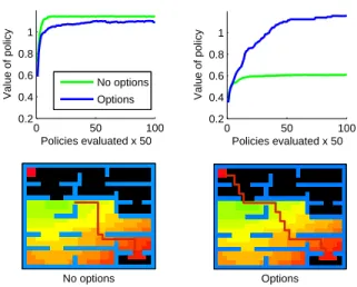
0 50 100 0.2 0.4 0.6 0.8 1 Policies evaluated x 50 Value of policy No options Options 0 50 100 0.2 0.4 0.6 0.8 1 Policies evaluated x 50 Value of policy No options Options

Figure 2: Results on the memory maze. Top left: with a shap-ing reward throughout the entire maze, usshap-ing options slightly degrades performance. Top right: when the shaping reward is turned off halfway through the maze, using options improves performance. The explanation is shown on the bottom row. Bottom left: path learned without using options (starting in the lower-right corner; the goal is in the upper-left corner). It consistently stops at the edge of the shaping reward without finding the goal. Bottom-right: options learned in the first half of the maze enable the agent to reliably find the goal.

In this domain, the agent has external, physical actions (denoted by ae ∈ AE) which move north, south, east and

west (here “AE” denotes “external action.”). Observations

are severely aliased, reflecting only the presence or absence of walls in the four cardinal directions (resulting in 16 possible observations, denoted oe∈ OE, for “external observation”).

To simultaneously capture state and a policy, we use a finite state controller (FSC). To allow for a potentially unbounded number of internal states, but to favor a small number a priori, we use a hierarchical Dirichlet Process prior. For every com-bination of internal state si ∈ SI and external observation

si, oe we choose a successor internal state from a Dirichlet

process. For ease of exposition, we will consider these to be internal, mental actions (denoted ai ∈ AI). The state of the

agent is therefore the joint state of the external observation and mental internal state.

The policy is a mapping from this joint state to both an internal action and an external action: π: SI× OE → AE×

AI. The prior for the internal mental states and actions is

θsi,oe ∼ GEM(α)

ae(si, oe) ∼ distribution over external actions

ai(si, oe) ∼ Multinomial(θsi,oe)

π(si, oe) = (ai(si, oe), ae(si, oe))

where GEM is the standard stick breaking construction of a DP over the integers [Pitman, 2002]. Note that we have ef-fectively created an HDP-HMM [Teh et al., 2006] with deter-ministic state transitions to model the FSC.

We now turn to the external actions. For each combination of internal state and external observation si, oe, we must

se-Figure 3: The snake robot (left), a learned policy for wiggling forward (middle), and the maze (right).

lect an action ae(si, oe). We take this opportunity to encode

more prior knowledge into our policy search. Because the maze is largely open, it is likely that there are repeated se-quences of external actions which could be useful—go north four steps and west two steps, for example. We term these

motor primitives, which are a simplified version of options

[Precup et al., 1998]. However, we do not know how long the motor primitives should be, or how many there are, or which sequence of actions each should be composed of.

Our distribution over motor primitives is given by the fol-lowing generative process: to sample a motor primitive k, we sample its length nk ∼ Poisson(λ), then sample nkexternal

actions from a compound Dirichlet-Multinomial.

Given the size of the search space, for our first experiment, we add a shaping reward which guides the algorithm from lower-right to upper-left. Figure 2 (upper left) compares the results of using motor primitives vs. not using motor primi-tives. The version with primitives does slightly worse.

The story changes significantly if we turn off the shaping reward halfway through the maze. The results are shown in the upper-right pane, where the option-based policy reliably achieves a higher return. The explanation is shown in the bottom two panes. Policies without options successfully learn a one-step north-west bias, but MCMC simply cannot search deeply enough to find the goal hidden in the upper-left.

In contrast, policies equipped with motor primitives consis-tently reach the goal. This is by virtue of the options learned as MCMC discovered good policies for the first half of the maze, which involved options moving north and west in large steps. These primitives changed the search landscape for the second half of the problem, making it easier to consistently find the goal. This can be viewed as a form of intra-task trans-fer; a similar story could be told about two similar domains, one with a shaping reward and one without.

4.3

Snakes in a (Planar) Maze: Adding

Continuous Actions

We now turn to our final experiment: controlling a simu-lated snake robot in a maze. This domain combines elements from our previous experiments: we will use a nonparamet-ric finite state controller to overcome partial observability, and attempt to discover motor primitives which are useful for navigation—except that low-level actions are now continu-ous and nine-dimensional. We will demonstrate the utility of

each part of our policy prior by constructing a series of in-creasingly complex priors.

The snake robot is shown schematically in Fig. 3. The snake has ten spherical segments which are connected by joints that move laterally, but not vertically. The snake is ac-tuated by flexing the joints: for each joint, a desired joint angle is specified and a low-level PD controller attempts to servo to that angle (the action space thus consists of a nine-dimensional vector of real numbers; joint angles are limited to ±45 degrees). As in a real snake, the friction on the segments is anisotropic, with twice as much friction perpendicular to the body (direction µ2 in Fig. 3) as along the body

(direc-tion µ1in Fig. 3). This is essential, allowing lateral flexing to

result in forward (or backward) motion.

The underlying state space is continuous, consisting of the positions, rotations, and velocities of the segments. This is all hidden; like the previous maze, observations only reflect the presence or absence of walls. Like the previous maze, there is a shaping reward.

4.4

Increasingly Complex Priors

Four priors were tested, with increasing levels of sophistica-tion. The first is a baseline “Flat, Uniform” model which at-tempts to directly sample a good external sequence of actions (ie, motor primitive) at every time t. There is no sharing of any sort here:

Model 1 (Flat Uniform):

π(t) ∼ distribution over smooth primitives

The second model attempts to learn reasonable motor primitives, which can be shared across different timesteps. We accomplish this with a Dirichlet Process prior that has a the smooth primitive distribution as its base measure. Thus, at every timestep t, the agent will sample an action sequence from the DP; with some probability, this will result in exe-cuting a previously-used motor primitive. Our policy search algorithm must now learn both the set of primitives and which one should be used at each timestep:

Model 2 (Flat w/DP):

θ ∼ DP(α, distribution over smoothprimitive)

π(t) ∼ θ

Neither of the first two models have an explicit notion of internal state. We now re-introduce the finite state con-troller, with a uniform distribution over motor primitives at each state:

Model 3 (FSC Uniform):

θe(si, oe) ∼ GEM(α)

ae(si, oe) ∼ distribution over external actions

ai(si, oe) ∼ Multinomial(θsi,oe)

π(si, oe) = (ai(si, oe), ae(si, oe))

Our final prior introduces sharing of the motor primitives among internal states, again by placing a Dirichlet Process prior over the motor primitives:

Model 4 (FSC w/DP):

θe(si, oe) ∼ GEM(α)

θi ∼ DP(α, distribution over smoothprimitive)

ae(si, oe) ∼ θi

ai(si, oe) ∼ Multinomial(θsi,oe)

π(si, oe) = (ai(si, oe), ae(si, oe))

The distribution over smooth primitives should encode our belief that some sequence of flexing will result in forward motion or motion around a corner, but we do not know the details. (In fact, no human attempting to interact with the simulator was able to move the snake at all!) We also believe that actions might be smoothly varying in time. To sample the sequence of actions for each primitive, we sample the first ac-tion uniformly from a nine-dimensional hypercube, and suc-cessive actions in the primitive are sampled recursively as a Gaussian drift around the previous action.

4.5

Results

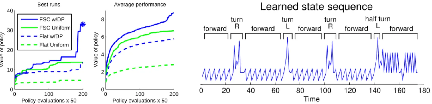
These four priors represent increasingly complex distribu-tions with complicated sharing of statistical strength among different policy elements. The results of executing our pol-icy search algorithm with each of the four priors is shown in Fig. 4 (middle). The figure plots average performance of using each prior, and is the key result of the paper: over time (horizontal axis), the quality of the policies increases (vertical axis). More complex policies yield better policies faster.

Importantly, our results show that as we add more layers to the hierarchy, the algorithm learns better and better poli-cies more quickly: FSCs perform better than non-FSC ver-sions, and priors with motor primitives perform better than non-motor-primitive versions. Why might this be so? Even though the models are increasingly complex, this complex-ity actually decreases the complexcomplex-ity of the overall search by allowing more and more opportunities to share statisti-cal strength. Thus, the flat models (i.e., with no sharing of motor primitives) must continually rediscover useful action sequences—a useful “wiggle forward” policy learned in the first part of the maze, must be re-learned in the second half. In contrast, the models with the Dirichlet Processes are able to globally reuse motor primitives whenever it is beneficial.

In Fig. 4 (left), we also plot the best runs of each of the four priors. In the 10,000 steps of inference allotted, only the FSC with primitives was able to navigate the entire maze (shown by reaching a reward of 33, highlighted with an as-terisk). Note in particular the striking “elbow” where the per-formance of our algorithm using Model 4 as a prior explodes: it is at this point where the algorithm has “figured out” all of the abstract structure in the domain, making it very easy to determine a complete optimal policy.

4.6

Examining what was learned.

In Fig. 4 (right) we examine the learned controller for one par-ticular run (this run made it about halfway through the maze). On the right is the learned sequence of states, which shows se-quences for wiggling forward, turning left, turning right, and executing a half turn when transitioning from the horizontal corridors to the vertical corridors.

0 100 200 0 10 20 30 40 Policy evaluations x 50 Value of policy Best runs 0 100 200 0 2 4 6 8 Policy evaluations x 50 Value of policy Average performance FSC w/DP FSC Uniform Flat w/DP Flat Uniform

Figure 4: Left: performance of different priors on the snake maze. Right: the learned state sequence.

12 different states were used in the FSC, but of those, the first four were used far more often than any others. These four allowed the snake to wiggle forward, and are shown in the middle of Fig. 3. Each state has a smooth primitive associated with it, of length 3, 3, 2 and 2, respectively (interestingly, the overall policy always used primitives of length 2, 3 or 6— never singleton primitives). Each external action is a nine-dimensional desired pose, which is plotted graphically and which demonstrates a smooth serpentine motion.

A video showing the learned policy is available at http://www.mit.edu/∼wingated/ijcai policy prior/

5

Conclusions

As planning problems become more complex, we believe that it will become increasingly important to be able to reliably and flexibly encode abstract prior knowledge about the form of optimal policies into search algorithms. Encoding such knowledge in a policy prior has allowed us to combine unsu-pervised, hierarchical Bayesian techniques with policy search algorithms. This combination accomplished three things: first, we have shown how we can express abstract knowl-edge about the form of a policy using nonparametric, struc-tured, and compositional distributions (in addition, the pol-icy prior implicitly expresses a preference ordering over poli-cies). Second, we have shown how to incorporate this abstract prior knowledge into a policy search algorithm based on a re-duction from planning to MCMC-based sampling. Third, we have shown how hierarchical priors can adaptively direct the search for policies, resulting in accelerated learning. Future work will address computational issues and push the algo-rithm to solve more challenging planning problems. We cur-rently use a generic probabilistic modeling language and in-ference algorithm; this genericity is a virtue of our approach, but special purpose engines could accelerate learning.

Acknowledgments

The authors gratefully acknowledge the financial support of AFOSR FA9550-07-1-0075 and ONR N00014-07-1-0937.

References

[Botvinick and An, 2008] Matthew Botvinick and James An. Goal-directed decision making in prefrontal cortex: a computational

framework. In Advances in Neural Information Processing

Sys-tems (NIPS), 2008.

[Gelly and Silver, 2008] Sylvain Gelly and David Silver. Achiev-ing Master Level in 9x9 Go. In National Conference on Articial

Intelligence (AAAI), 2008.

[Goodman et al., 2009] Noah D. Goodman, Tomer Ullman, and Joshua B. Tenenbaum. Learning a theory of causality. In

Pro-ceedings of the Thirty-First Annual Conference of the Cognitive Science Society, 2009.

[Howard, 1960] Ronald A. Howard. Dynamic Programming and

Markov Processes. The MIT Press, Cambridge, Massachusetts,

1960.

[Kaelbling et al., 1998] Leslie P. Kaelbling, Michael L. Littman, and Anthony R. Cassandra. Planning and acting in partially ob-servable stochastic domains. Artificial Intelligence, 101:99–134, 1998.

[Lazaric et al., 2007] Alessandro Lazaric, Marcello Restelli, and Andrea Bonarini. Reinforcement Learning in Continuous Action Spaces through Sequential Monte Carlo Methods. In Advances

in Neural Information Processing Systems (NIPS), 2007.

[Pitman, 2002] Jim Pitman. Poisson-Dirichlet and GEM invari-ant distributions for split-and-merge transformations of an in-terval partition. Combinatorics, Probability and Computing,

11:501514, 2002.

[Precup et al., 1998] Doina Precup, Richard S. Sutton, and Satinder Singh. Theoretical results on reinforcement learning with tem-porally abstract options. In European Conference on Machine

Learning (ECML), pages 382–393, 1998.

[Teh et al., 2006] Yee Whye Teh, Michael I. Jordan, Matthew J. Beal, and David M. Blei. Hierarchical Dirichlet processes.

Journal of the American Statistical Association, 101:1566–1581,

2006.

[Toussaint et al., 2006] Marc Toussaint, Stefan Harmeling, and Amos Storkey. Probabilistic inference for solving (PO)MDPs. Technical Report EDI-INF-RR-0934, University of Edinburgh, 2006.

[Toussaint et al., 2008] Marc Toussaint, Laurent Charlin, and Pas-cal Poupart. HierarchiPas-cal POMDP Controller Optimization by Likelihood Maximization. In Uncertainty in Artificial

Intelli-gence, 2008.

[Williams, 1992] R. Williams. Simple statistical gradient-following algorithms for connectionist reinforcement learning. Machine