The Bayesian validation metric : a framework for probabilistic model calibration and validation

(1)

The Bayesian Validation Metric: A Framework for

Probabilistic Model Calibration and Validation

by

Tony Tohme

Submitted to the Center for Computational Science and Engineering

in partial fulfillment of the requirements for the degree of

Master of Science in Computation for Design and Optimization

at the

MASSACHUSETTS INSTITUTE OF TECHNOLOGY

May 2020

c

○ Massachusetts Institute of Technology 2020. All rights reserved.

Author . . . .

Center for Computational Science and Engineering

May 20, 2020

Certified by . . . .

Kamal Youcef-Toumi

Professor of Mechanical Engineering

Thesis Supervisor

Accepted by . . . .

Youssef Marzouk

Associate Professor of Aeronautics and Astronautics

Co-Director, Center for Computational Science and Engineering

(2)

(3)

The Bayesian Validation Metric: A Framework for

Probabilistic Model Calibration and Validation

by

Tony Tohme

Submitted to the Center for Computational Science and Engineering on May 20, 2020, in partial fulfillment of the

requirements for the degree of

Master of Science in Computation for Design and Optimization

Abstract

In model development, model calibration and validation play complementary roles toward learning reliable models. In this thesis, we propose and develop the “Bayesian Validation Metric” (BVM) as a general model validation and testing tool. We show that the BVM can represent all the standard validation metrics – square error, reliability, probability of agreement, frequentist, area, probability density comparison, statistical hypothesis testing, and Bayesian model testing – as special cases while improving, generalizing and further quantifying their uncertainties. In addition, the BVM assists users and analysts in designing and selecting their models by allowing them to specify their own validation conditions and requirements. Further, we expand the BVM framework to a general calibration and validation framework by inverting the validation mathematics into a method for generalized Bayesian regression and model learning. We perform Bayesian regression based on a user’s definition of model-data agreement. This allows for model selection on any type of data distribution, unlike Bayesian and standard regression techniques, that “fail” in some cases. We show that our tool is capable of representing and combining Bayesian regression, standard regression, and likelihood-based calibration techniques in a single framework while being able to generalize aspects of these methods. This tool also offers new insights into the interpretation of the predictive envelopes in Bayesian regression, standard regression, and likelihood-based methods while giving the analyst more control over these envelopes.

Thesis Supervisor: Kamal Youcef-Toumi Title: Professor of Mechanical Engineering

(4)

(5)

(6)

(7)

Acknowledgments

This research was performed collaboratively with Dr. Kevin Vanslette under the supervision of Professor Kamal Youcef-Toumi, and it was generously supported by the Center for Complex Engineering Systems (CCES) at King Abdulaziz City for Science and Technology (KACST) and the Massachusetts Institute of Technology (MIT).

I would like to express my sincere gratitude and deep appreciation to Kamal for believing in me and inspiring me. His guidance and support have been invaluable throughout this research.

Much credit for the work in this thesis goes to my fantastic friend, collaborator, and mentor Kevin. His motivation and encouragement have been the driving force behind this research. I honestly owe him tremendously.

I am highly indebted to Associate Provost Philip Khoury whose inspiration and support made my journey at MIT superb and fruitful.

I was very fortunate to take a course with Professor Gilbert Strang. I am genuinely blessed to have worked with him.

Many thanks to Professor Youssef Marzouk, Professor Nicolas Hadjiconstantinou, and Kate Nelson for being behind the success of the Center for Computational Science and Engineering (CCSE).

I am profoundly grateful to Tariq, Kathy, and my friends for being there for me and celebrating with me every success.

Finally, words will never be enough to express my gratitude and love to my parents, Mike and Nicole, my girlfriend Maria, my uncles, Georges and Ziad, my aunts, Simone, Mona and Arlette, my granduncle Emile, and my grandparents, Salma, Yvette and Pierre, for their endless support, encouragement, sacrifices and love; this thesis is dedicated to them. Lastly, yet most importantly, I would like to thank God who has given me the insight, strength, and perseverance to complete this work.

(8)

(9)

A Note on the Content

This thesis contains material which I authored or co-authored [58, 62]. Chapter 2 of this thesis is based on the following previous publication:

[62] Kevin Vanslette, Tony Tohme, and Kamal Youcef-Toumi. A general model validation and testing tool. Reliability Engineering & System Safety, 195, March 2020.

Chapter 3 of this thesis is based on the following manuscript:

[58] Tony Tohme, Kevin Vanslette, and Kamal Youcef-Toumi. Generalized bayesian regression and model learning. arXiv preprint arXiv:1911.11715, 2019.

(10)

(11)

List of Figures

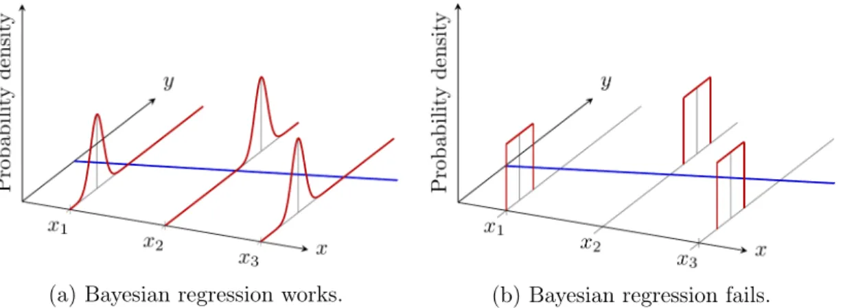
1-1 Illustrative example of theoretical success and failure cases of Bayesian regression. In blue is a deterministic linear model (𝑦 = 𝑎𝑥 + 𝑏) and in red are the data probability distributions that may come from epistemic and/or aleatoric uncertainty. . . 26 2-1 A common model validation scenario. The model line is trained on

noisy data (not depicted in the figure) and is to be compared to a set of validation data. As both the model line and the data are uncertain in general, any quantitative measure (i.e. the comparison function) between these comparison values inherits this uncertainty. Thus, any accept/reject rule on the basis of these uncertain comparison function values is uncertain as well. A visual inspection of this graph seems to indicate, up to statistical fluctuation, that the comparison values of the model and data more or less (or probably) agree, but this intuitive measure has yet to be quantified. Graphic adapted from [44]. . . 30

(16)

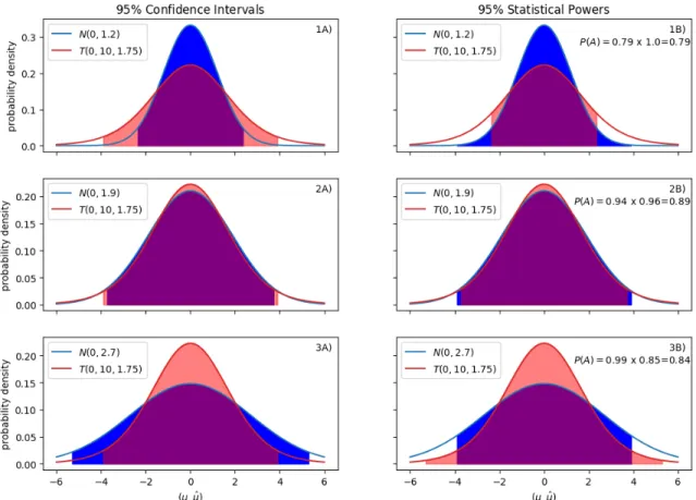
2-2 Comparison between statistical hypothesis testing and statistical power BVM. (a) The shaded regions in Column A depict the 95% confidence interval of each distribution, respectively. Because the data distribution is the same in each figure and because the statistical hypothesis test is independent of the proposed model due to assuming the hypothesis 𝑀 = 𝐷, each model is equally valid by that test when it is clear that the model in row 2 is preferable. (b) The shaded regions in Column B depict the statistical power of the distributions – the 95% confidence intervals from each distribution is shaded (integrated) in the other’s pdf. The statistical power BVM (denoted 𝑃 (𝐴) in column B) is calculated for each model and indeed the model in row 2 is found to be preferable as it has the highest probability of agreement. . 47 2-3 Validating a deterministic model and an uncertain model

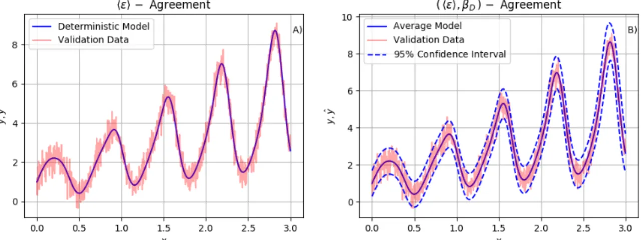
accord-ing to two Boolean agreement functions. (a) The deterministic model satisfies the ⟨𝜖⟩ Boolean but fails to pass the(︀⟨𝜖⟩, 𝛽𝐷)︀ requirement given that

its 95% confidence interval has a width of zero. (b) The uncertain model satisfies both the ⟨𝜖⟩ and(︀⟨𝜖⟩, 𝛽𝐷)︀ agreement requirements given that its 95%

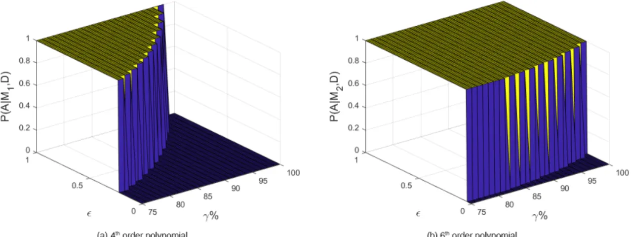
confidence region has a nonzero width and represents better the uncertain data. . . 49 2-4 Completely Certain Case: The BVM probability of agreement

be-tween each of the models and data plotted in the (𝛾, 𝜖) space. Be-cause here the models are deterministic, the BVM probability of agreement for each (𝛾, 𝜖) pair is either zero or one. (a) The results for model 1 (4th

order polynomial). (b) The results for model 2 (6th _{order polynomial). As}

expected, model 2 better fits the data in the (𝛾, 𝜖) space as it has more BVM values equal to one than model 1, since it is overall closer to the cosine function being the next nonzero order polynomial in the Taylor series expansion. Neither model fits the data exactly as the BVM for both models at (𝛾 = 100%, 𝜖 = 0) is zero. . . 53

(17)

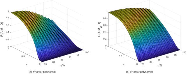
2-5 Uncertain Case: The BVM probability of agreement between each of the models and the data plotted in the (𝛾, 𝜖) space. Because the model paths are uncertain, the BVM probability of agreement for each (𝛾, 𝜖) pair may take any value from zero to one. (a) The results for model 1 (4th

order polynomial). (b) The results for model 2 (6th _{order polynomial). As}

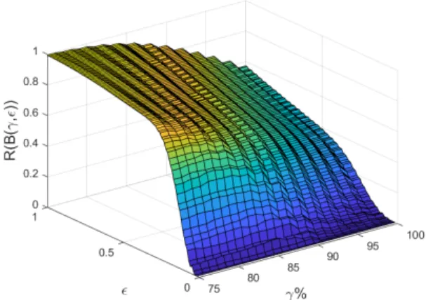
expected, model 2 better fits the data in the (𝛾, 𝜖) space as it has generally larger BVM values than model 1; however, the BVM values are about equal in cases of large values of 𝜖 and low values of 𝛾 (since the definition of agreement is less stringent and they both “agree”) and in the case of demanding absolute equality (𝜖 = 0) as neither model fits the data exactly. . . 54 2-6 The BVM ratios for the uncertain models plotted in the (𝛾, 𝜖) space.

Model 2 is generally favored over model 1 as there exist no values greater than one on the plot. The amount the BVM ratio favors model 2 over model 1 decreases (i.e. the ratio increases and tends to one) as the metric becomes less and less stringent (i.e. as 𝛾 decreases and 𝜖 increases). The 𝜖 = 0 line was removed because neither model agrees with the data exactly. . . 55 3-1 Truncated tail data distributions solution. Using BVM regression

re-sults in a nonzero probability of finding a model given the observed truncated data. . . 68 3-2 Predictive envelopes of the model in the absence of data

uncer-tainty using the BVM. As tabulated in Table 3.3, Bayesian regression fails to produce a candidate model solution as the data is completely certain and standard regression produces a single deterministic solution with no model uncertainty. . . 72

(18)

3-3 Illustration of BVM Learning for the Monod model for decreasing values of 𝜖. In the first row is the prior/posterior parameter distribution in (𝛼1, 𝛼2) space. The data points are shown by a blue circle in the second

row. The first column corresponds to the situation before any data point is observed and shows a plot of the prior distribution in (𝛼1, 𝛼2) space together

with six samples of the model response 𝑀 (𝑥; ⃗𝛼) (red lines) in which the values of 𝛼1 and 𝛼2 are randomly drawn from the prior. In the second, third

and fourth columns, we see the situation after running our BVM learning using MCMC, with a tolerance 𝜖 = 0.03, 𝜖 = 0.025 and 𝜖 = 0.02, respectively. The posterior has now been influenced by the agreement tolerance 𝜖, this gives a relatively compact posterior distribution. Samples from this posterior distribution lead to the functions shown in red in the second row. . . 73 3-4 Comparison between Bayesian regression and BVM regression. (a)

Bayesian regression under infinite tail data distribution. Note that the 95% confidence interval is very narrow and standard regression method produces a nearly identical result. (b) BVM regression using the compound Boolean. In this case, the 95% confidence region is much wider and represents the data more accurately. Note that this probabilistic model passes both agreement conditions imposed by the compound Boolean 𝐵( ^𝑌 , 𝑌, ⟨𝜖⟩, ^𝛼). Starting with a very small ⟨𝜖⟩ in the MCMC simulation, we tune ⟨𝜖⟩ by gradually increasing its value until both elements of the compound Boolean are naturally satisfied. 76

(19)

List of Tables

2.1 Specification of the four BVM inputs that give the other validation metrics as special cases. The column headings are the four BVM input values: Comparison Values (^𝑧, 𝑧), Probabilities (𝜌(^^ 𝑧|𝑀, 𝐷), 𝜌(𝑧|𝐷)), Comparison Function 𝑓 = 𝑓 (^𝑧, 𝑧), and the Boolean Agreement Function 𝐵(𝑓 ). The row headings read: Reliability, Improved Reliability, Frequentist, Area, Pdf Comparison Metrics, Statistical Hypothesis Testing, and Bayesian Model Testing. The denoted data probability for the average in the frequentist metric, Stud. 𝑡, is the Student’s 𝑡-distribution. . . 40 2.2 BVM representation of the other validation metrics as special cases using

the comparison functions (the 𝑓 ’s) specified in Table 2.1. . . 41 3.1 Some examples of agreement Boolean functions. . . 67 3.2 The observations we aim to fit. . . 70 3.3 High probability of the model producing posterior parameter distributions and

predictive envelopes for different types of data distributions using the three approaches. BVM regression is capable of producing posterior distributions of the model parameters for any type of data distributions. . . 71

(20)

(21)

Chapter 1 Introduction

1.1 Introduction and Overview

Engineering systems are often represented and described by computational models in order to make predictions about the behavior of the system. Often, models possess parameters that cannot be directly measured, and instead they are inferred based on experimental data of relevant inputs and outputs, in a process known as model calibration [22,36,60,65]. Model calibration is the process of estimating and adjusting model parameters to obtain a model representation of the system (or data) of interest while satisfying a specific criterion (objective function). Once the parameters are inferred, the designed model is tested with respect to real data-generating process, in a task known as model validation [39, 55,60].

In model development, model calibration comes in the stage prior to the validation stage [52], and it usually consists of estimating model parameters given a set of observed input-output data. Then, validation is performed on a different independent data set called the validation data set. In what follows, we will use the terms “model calibration”, “model learning” and “regression” interchangeably.

We are interested in studying the calibration and validation of multivariate com-putational models that represent uncertain situations and observations (or data). It is understood that complete certainty is a special case of uncertainty as both may be represented with probability distributions.

(22)

The uncertainty in a model or data set may originate from stochasticity, model parameter and input data uncertainty, measurement uncertainty, or other possible aleatoric or epistemic sources of uncertainty. Each of the following data modeling schemes may include quantifiable amounts of uncertainty (or certainty) that we would like to calibrate and then validate on the basis of a set of calibration and validation data: neural networks and AI models, machine learning models, Gaussian Process Regression models [18], polynomial chaos and other surrogate models [1, 7,15, 21], spatial and time series stochastic models, physics based models (usually solutions to differential equations), engineering based models (which are sufficiently abstracted physics based models), Monte Carlo simulation models [16,35], and more. Model output uncertainties may be quantified through uncertainty propagation techniques (that may or may not include verification, calibration, and validation) [1,7,15,18,25,31,41,49,50,52,56].

1.2 Related Work

Model calibration techniques have been widely studied in the literature. Least squares (or standard regression) [64], likelihood-based [9,43], and Bayesian regression methods [23, 24, 32, 40,63] are often used for model parameter estimation. Nonprobabilistic methods, such as parametric model regression, nonparametric neural networks, and support vector machines (SVM) [4] are able to tackle these types of problems efficiently. In Bayesian probability theory [29, 30, 53], Bayesian model testing and maximum likelihood methods provide probabilistic features (i.e. mean, covariance, distribution) for the parameters we aim to estimate, based on prior knowledge (i.e. prior distribution) and the uncertainty of the data. Bayesian model testing, which uses Bayesian parameter regression, was shown to be successful for signal detection, light sensor characterization [20], exoplanet detection [46], extra-solar planet detection [45], laser peening process [40], time series [59], astronomical data analyses [10], and cosmology and particle physics [11].

Model validation techniques have also been extensively studied in the literature. There exist several validation metrics. Each metric is designed to compare features of

(23)

a model-data pair to quantify validation: square error compares the difference in the data and model values in a point to point or interval fashion [63], the reliability metric [47] and the probability of agreement [57] compare continuous model outputs and data expectation values (the model reliability metric was extended past expectation values in [51]), the frequentist validation metric [38] and statistical hypothesis testing compare data and model test statistics, the area metric compares the cumulative distribution of the model to the estimated cumulative distribution of the data [12,26,27,49,65,67], probability density function (pdf) comparison metrics (such as the KL Divergence) measure and represent “closeness” between pdfs, and Bayesian model testing compares the posterior probability that each model would correctly output the observed data [13, 14, 31, 45, 50, 53, 66]. A detailed review of the majority of these metrics may be found in [22, 28,34, 36] and the references therein. In particular, [34] is an up to date review that considers many validation metrics in the cases of data and model certainty, data uncertainty and model certainty, and data and model uncertainty.

To assist the comparison of the positive and negative aspects of the above validation metrics, reference [28] outlines six “desirable validation criteria” that a validation metric might have (they extend [12, 38]). One conclusion from [28] is that none of the available metrics simultaneously satisfy all six desirable validation criteria. We summarize the most important features of the desirable validation criteria with the following validation criterion:

1. A validation metric should be a statistically quantified quantitative measure (as opposed to a qualitative measure) of the agreement between (general) model predictions and data pairs, in the presence or absence of uncertainty.

The desire for objectivity, “that a metric will produce the same assessment for every analyst independent of their individual preferences” [28], is difficult to satisfy because there are no rules in place to guide a modeler toward selecting one validation metric over another. For this reason, the individual might simply choose a metric based on their preferences, or worse, be tempted to base their decision on which validation metric gives them the most favorable evaluation. Given individuals may choose

(24)

different validation metrics for the same model-data pair, it is possible for individuals to impose accuracy requirements that are incompatible with one another and arrive at different conclusions regarding the validity of the same model-data pair. As the final goal is objectivity, when possible, a map between the accuracy requirements should be constructed such that the validation metrics yield consistent evaluations of the model-data validity when applicable.

Further, Liu et al. [28] suggest that there is no agreed upon unified model-data comparison function. Even including the results of this thesis, we expect this statement to hold as it is extremely difficult to guess the prior information about the utility of a model an analyst may be required to include in the validation of a model-data pair. For instance, given arbitrary data, “What features of the data are relevant to capture with a model?”, “Of these features, are some more relevant than others?”, and “What accuracy is required for the model to be valid?”. Agreement and validation are ultimately human-made concepts designed for the purpose of expressing that “in general, not every feature or statistic between a model-data pair need to be equal to conserve the utility of the model”. For some model-data pairs, all that may be required is that the model and data averages closely match within uncertainty, while for others, one may require that the model can accurately reproduce the probability distribution of a data set as a whole (as one would do to physically model a noisy measurement device). Given the wide variety of data and the large number of different inferences (and thus models and hypotheses) that one may be interested in drawing from a given data source (i.e. the context of the model-data pair), we do not expect any single set of comparison functions, statistics, or values to be equally relevant and maximally useful for all possible model-data contexts. This, however, does not stop us from quantifying the validity of a model-data pair given any arbitrary comparison function and with any arbitrary definition of agreement.

(25)

1.3 Objectives and Contributions

In this thesis, we propose and construct the “Bayesian Validation Metric” (BVM) as a general model validation and testing tool. We design the BVM to adhere to the desired validation criterion (1.) by using “four BVM inputs”: the model and data comparison values, the model output and data pdfs, the comparison value function, and the agreement function. The comparison value function is a function of model output and data comparison values that provides the desired quantitative comparison measure, e.g. square difference. Using the model output pdf and the data pdf, the value of the comparison value function is statistically quantified. In turn, the agreement function provides an accept/reject rule and effectively wraps the previous three BVM inputs together to give the BVM. From this, the BVM outputs “the probability the model and data agree”, where agreement is a user-defined Boolean function that meets, or does not meet, accuracy requirements between model and data comparison values. Thus, the BVM meets the desired validation criterion (1.) for arbitrary comparison value functions, arbitrary definitions of agreement, and in principle for arbitrary data types such as integers, vectors, tensors, strings, pictures, or others.

The BVM can be used to represent all of the aforementioned validation metrics as special cases. We find the conditions under which several of the current validation metrics are effectively equal to one another, which improves the objectivity of the current validation procedure. In brief we find that the frequentist metric (using natural definitions of agreement) is equal to the reliability metric and the probabilities from Bayesian model testing are equal to the probabilities of the improved model reliability metric [51] when one demands exact equality of the (uncertain) model-data comparison values. Because probability can represent both certain and uncertain situations, so can the BVM. Thus, these “special case” metrics can be generalized to quantify certain or uncertain cases, and even be combined into more complex validation requirements using the BVM framework. Thus, the BVM provides a standardized framework to improve, generalize, or further quantify these validation metrics.

(26)

frame-work [53], in which one constructs the Bayes ratio to rank models according to the ratio of their posterior probabilities given the data. We show that these posterior probabilities are equal to a special case of the BVM under the definition of agreement that requires these uncertain model outputs and data to match exactly. Thus, nothing prevents us from extending the logic used in the Bayesian model testing framework to our framework and we construct the BVM ratio for the purpose of model selection under arbitrary definitions of agreement, i.e. for arbitrary validation scenarios.

Moving to Bayesian calibration techniques, we believe that the efficacy of para-metric Bayesian regression, likelihood-based methods, and standard regression can be improved. Bayesian regression calculates the Bayesian evidence, which is the proba-bility the model could have produced the observed, usually over noisy or uncertain, data. If this probability is nonzero, one can proceed to calculate posterior model parameter probabilities using Bayes’ Theorem. In practice, there are models and parameters that may be of interest to the user that Bayesian regression fails to regress and produce posterior parameter distributions – Figure 1-1. For some of the instances that Bayesian regression fails to provide a solution, standard regression may actually succeed, but usually with some measure of expected error. How this error can translate into parameter and model uncertainty in the presence of certain or uncertain data is a problem that is largely omitted in the literature except for a few analytic cases.

(a) Bayesian regression works. (b) Bayesian regression fails.

Figure 1-1: Illustrative example of theoretical success and failure cases of Bayesian regression. In blue is a deterministic linear model (𝑦 = 𝑎𝑥 + 𝑏) and in red are the data probability distributions that may come from epistemic and/or aleatoric uncertainty.

(27)

Figure 1-1a shows normally distributed data (infinite tails data distribution). In this case, parametric Bayesian regression finds a linear model that sits in low probability regions of the data. Figure 1-1b shows uniformly distributed data (truncated data distribution). In this case, Bayesian regression cannot find a linear model solution because no linear model can pass through each data distribution simultaneously – the model given the data is regarded as impossible. Standard regression methods can provide linear model solutions here despite the model lying in a zero probability region of the data. Although this solution may be considered “wrong” because it is not supported by the data, it successfully provides useful information to the modeler (an increasing trend). The fact that, for the same model, the solution given by the calibration method can differ from method to method supports the search for a framework for their joint representation so they may be compared more concretely.

In this thesis, we represent least squares, likelihood-based, and Bayesian regression (or calibration) methods by expanding the general validation framework (BVM) into a general calibration and validation framework. Our method uses the BVM to guide the regression of a model in a flexible way. Several of our examples use generalizations of the improved reliability metric and thus reliability is automatically regressed into our model solutions. Our method gives us better control over the predictive envelopes of the model under question, which can be used to improve model reliability and safety. By learning model parameters with the BVM, we are able to estimate and construct model parameters distributions for any type of data distribution (Gaussian, Uniform, Completely Certain), which addresses the concerns raised in Figure 1-1. This construction gives us additional insight into the meaning of the predictive envelopes of Bayesian regression methods.

We have found that a subset of our method shares mathematical features with Ap-proximate Bayesian Computation (ABC) methods, which are also known as likelihood-free techniques [2, 33]. ABC methods are used strictly as an approximation method for nearly computationally intractable likelihoods in Bayesian regression. While our method gains this feature in some cases, our method’s intention is not to approximate Bayesian regression, but instead to generalize it for the purpose of robust and flexible

(28)

model calibration.

Our method is able to regress models over a multitude of different data distributions by using likelihoods that are modified by user’s choice of a useful definition of agreement between the data and the model – leaning on the BVM formalism. This “choice” allows the user to program safety requirements into the model learning process if they desire. The nature of the BVM formalism forces one to express the model and data assumptions explicitly and thus our method leads to improved model transparency and safety. In our examples we show how such a procedure leads to a model that better represents the uncertain data at hand than Bayesian and standard regression techniques. This naturally improves the model’s reliability and safety in the presence of uncertain data.

1.4 Thesis Outline

The remainder of the thesis is organized as follows. In Chapter 2, we derive and construct the BVM by following our validation criterion. Through some edge cases, we show that the BVM satisfies both the six desirable validation criteria from [28] as well as our validation criterion (1.). We also summarize the results derived in Appendix A, where we incorporate all of the above standard validation metrics as special cases of the BVM, draw relationships between several of the validation metrics, provide improvements and generalizations to these metrics as is suggested by the functional form of the BVM, and construct the BVM ratio. We end the chapter by representing three novel validation metrics using the BVM and comparing them to similar metrics from the literature. We then move to Chapter 3, where we employ the BVM framework to generalize Bayesian regression. This generalized Bayesian regression method, namely the BVM model learning technique, works for different types of data distributions and for arbitrary definitions of model-data agreement. We then present a simulation application using the BVM model learning technique on a nonlinear heuristic model, along with a compound Boolean agreement function example. Chapter 4 is left for conclusions and recommendations.

(29)

Chapter 2 The Bayesian Validation Metric

2.1 Introduction

In this chapter, we introduce and develop the Bayesian Validation Metric (BVM) which is a general model validation and testing tool [62]. We find the BVM to be capable of representing all of the well-known validation metrics as special cases, while improving, generalizing and further quantifying their uncertainties. The BVM has the capacity to allow users to invent and select models according to novel validation requirements. We formulate and test a few novel compound validation metrics that improve upon other validation metrics in the literature. In addition, we propose and construct the BVM Ratio for the purpose of quantifying model selection under user-specified definitions of model-data agreement in the presence or absence of uncertainty. This construction generalizes the Bayesian model testing framework.

2.2 Notation and Overview

For the remainder of the thesis, we will use the following notation and language. We will let ^𝑦 denote the output of a model, ^𝑌 = {^𝑦1, ..., ^𝑦𝑛} a set of 𝑛 model outputs, 𝑦 a data

point (or observed data), and 𝑌 = {𝑦1, ..., 𝑦𝑛} a set of 𝑛 data points. The proposition

𝑀 essentially stands for “the model” or “coming from the model”, i.e. ^𝑦 = 𝑀 (𝑥; ⃗𝛼), where 𝑥 is the input and ⃗𝛼 = (𝛼1, . . . , 𝛼𝑚) represents a vector of 𝑚 model parameters.

(30)

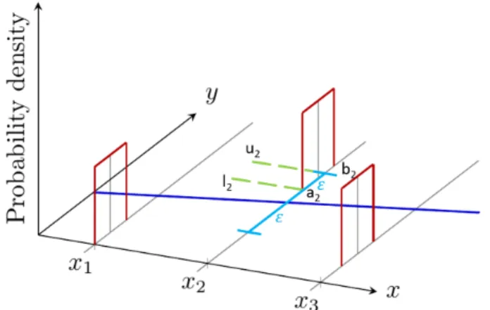
The proposition 𝐷 stands for “the experiment” or “coming from the experiment”. We let ^𝑧 and 𝑧 represent the comparison quantities of interest, which pertain to the model and the data respectively. Further, we let the comparison quantities take general forms, such as multidimensional vectors, functions, or functionals (e.g. output values, expectation values, pdfs, ...), so we can represent any such pair of quantities we may wish to compare between the model and the data. When we refer to “the four BVM inputs” we mean: the comparison values (^𝑧, 𝑧), the model output and data pdf 𝜌(^𝑧, 𝑧|𝑀, 𝐷), the comparison value function 𝑓 (^𝑧, 𝑧), and the agreement function 𝐵 = 𝐵(𝑓 (^𝑧, 𝑧)). The (denoted) integrals may be integrals or sums depending on the nature of the variable being summed or integrated over, which is to be understood from the discrete or continuous context of the inference at hand. The dot “ · ” represents standard multiplication, which is mainly used to improve aesthetics. Finally, we let 𝐴 denote the agreement between the model output and the observed data.

Figure 2-1: A common model validation scenario. The model line is trained on noisy data (not depicted in the figure) and is to be compared to a set of validation data. As both the model line and the data are uncertain in general, any quantitative measure (i.e. the comparison function) between these comparison values inherits this uncertainty. Thus, any accept/reject rule on the basis of these uncertain comparison function values is uncertain as well. A visual inspection of this graph seems to indicate, up to statistical fluctuation, that the comparison values of the model and data more or less (or probably) agree, but this intuitive measure has yet to be quantified. Graphic adapted from [44].

(31)

Performing uncertainty propagation through a model results in a model output probability (density) distribution 𝜌(^𝑦|𝑀, 𝐷) that ultimately we would like to validate by comparing it to an uncertain validation data source 𝜌(𝑦|𝐷), to see if they agree (as depicted in Figure 2-1). The immediate question is, however, “What values do we want to compare and what do we mean by agree?”. Given the wide variety of data and the large number of different inferences (and thus models and hypotheses) that one may be interested in drawing from a given data source (i.e. the context of the model-data pair), we do not expect any single set of comparison functions to be equally relevant and maximally useful for all possible model-data contexts. In light of this, we instead quantify the validity of a model-data pair given any arbitrary comparison value function and according to any arbitrary definition of agreement.

2.3 Formulation of the BVM

In this section, we construct the Bayesian Validation Metric (BVM), we show its different representations, and we discuss its importance and statistical responsibility.

2.3.1 Derivation

Here we start constructing the Bayesian Validation Metric (BVM). To capture the concept of what we might mean by agree, we define ^𝑧 and 𝑧 to agree, 𝐴, when the Boolean expression, 𝐵, is true. Both 𝐴 and 𝐵 are defined by the modeler and their prior knowledge of the context of the model-data pair. Naturally then, the agreement function 𝐵 = 𝐵(︀𝑓 (^𝑧, 𝑧))︀ = 𝐵(^𝑧, 𝑧) is some function or functional of a comparison value function 𝑓 (^𝑧, 𝑧).

Given the values of ^𝑧 and 𝑧 are known, i.e. certain, we quantify agreement using a probability distribution that assigns certainty,

𝑝(𝐴|^𝑧, 𝑀, 𝑧, 𝐷) = Θ(︀𝐵(^𝑧, 𝑧))︀. (2.1)

(32)

“agreeing”) and equal to zero otherwise. Thus, in the completely certain case, we are certain as to whether the model and data comparison values agree or do not agree, as defined by 𝐵 and the deterministic evaluation of 𝑓 (^𝑧, 𝑧).1 _{We will call 𝑝(𝐴|^}_{𝑧, 𝑀, 𝑧, 𝐷)}

the “agreement kernel”.

Given that in general the comparison values are uncertain, and quantified by 𝜌(^𝑧, 𝑧|𝑀, 𝐷), the probability the comparison values agree, as defined by 𝐵 and 𝑓 (^𝑧, 𝑧), is equal to, 𝑝(𝐴|𝑀, 𝐷) = ∫︁ ^ 𝑧,𝑧 𝑝(𝐴|^𝑧, 𝑀, 𝑧, 𝐷) · 𝜌(^𝑧, 𝑧|𝑀, 𝐷) 𝑑^𝑧 𝑑𝑧, (2.2) 𝑖𝑛𝑑. −→ ∫︁ ^ 𝑧,𝑧 𝜌(^𝑧|𝑀, 𝐷) · Θ(︀𝐵(^𝑧, 𝑧))︀ · 𝜌(𝑧|𝐷) 𝑑^𝑧 𝑑𝑧, (2.3)

which is a marginalization over the spaces of (^𝑧, 𝑧).2 _{Equation (2.2) is the general}

form of the Bayesian Validation Metric (BVM). Because 𝐴 is discrete, the BVM is a probability rather than a probability density and it therefore falls in the range 0 ≤ 𝑝(𝐴|𝑀, 𝐷) ≤ 1. Equation (2.3) explicitly assumes that the uncertainty in the data is independent of the model, i.e. 𝜌(𝑧|𝑀, ^𝑧, 𝐷) = 𝜌(𝑧|𝐷), that the data 𝐷 does not take ^𝑧 or the model 𝑀 (that it is currently being compared to) as inputs.3 This is a relatively common scenario so it is stated explicitly. The BVM may be computed using any of the well-known computational integration methods.

1_{This binary yet probabilistic definition of agreement turns out to be completely satisfactory for} our current purposes. As is briefly discussed later, the sharp boundaries of the indicator function can be smoothed out without employing fuzzy logic by allowing parameters in the Boolean function to themselves be uncertain and marginalized over.

2_{Recall that the propositions in the probability distributions 𝜌(𝑧|𝐷) and 𝜌(^}_{𝑧|𝑀, 𝐷) are completely} arbitrary (in some cases requiring propagation from 𝜌(𝑦|𝐷) and 𝜌(^𝑦|𝑀, 𝐷)), they could be both continuous, discrete (with order), categorical variables (no well defined order, e.g. strings, pictures,...), or a mix.

3_{In a controls system this may not be the case, as the model may interact with the system of} interest. In such a case this constraint may be lifted and one should use (2.2) instead. The joint probability 𝜌(^𝑧, 𝑧|𝑀, 𝐷) can be used to account for the correlations between the model (the controller or reference) and the data (the measured response of the system being controlled) in a controls setting in principle.

(33)

2.3.2 An Identical Representation

In some cases, it is useful to work directly with the probability density 𝜌(𝑓 |𝑀, 𝐷), which quantifies the probability the comparison value function 𝑓 (^𝑧, 𝑧) takes the value 𝑓 due to uncertainty in its inputs. This pdf is independent of any user-defined accuracy requirement. We will call this pdf the comparison value probability density, which is equal to, 𝜌(𝑓 |𝑀, 𝐷) = ∫︁ ^ 𝑧,𝑧 𝛿(𝑓 − 𝑓 (^𝑧, 𝑧)) · 𝜌(^𝑧, 𝑧|𝑀, 𝐷) 𝑑^𝑧 𝑑𝑧. (2.4)

This is the net uncertainty propagated through the comparison value function 𝑓 (^𝑧, 𝑧) from the uncertain model and data comparison values. All of the expectation values that are associated with 𝑓 may be generated from this pdf.

If one imposes an accuracy requirement with a Boolean expression 𝐵 = 𝐵(𝑓 ) (i.e. defining agreement according to the value of 𝑓 ), the resulting accumulated prob-ability is the BVM. That is, the BVM, i.e. Equation (2.2), may equally be expressed as,

𝑝(𝐴|𝑀, 𝐷) = ∫︁

𝑓

𝜌(𝑓 |𝑀, 𝐷) · Θ(︀𝐵(𝑓 ))︀ 𝑑𝑓, (2.5)

which is proven through substitution and marginalization over 𝑓 ,

𝑝(𝐴|𝑀, 𝐷) = ∫︁ 𝑓 (︁∫︁ ^ 𝑧,𝑧 𝛿(𝑓 − 𝑓 (^𝑧, 𝑧)) · 𝜌(^𝑧, 𝑧|𝑀, 𝐷) 𝑑^𝑧 𝑑𝑧)︁· Θ(𝐵(𝑓 )) 𝑑𝑓 = ∫︁ ^ 𝑧,𝑧 Θ(𝐵(^𝑧, 𝑧)) · 𝜌(^𝑧, 𝑧|𝑀, 𝐷) 𝑑^𝑧 𝑑𝑧. (2.6)

2.3.3 Importance and Statistical Responsibility

The BVM allows the user to, in principle, quantify the probability the model and the data agree with one another under arbitrary comparison value functions and with arbitrary definitions of agreement. The BVM can therefore be used to fully quantify the probability of agreement between arbitrary model and data types using novel or existing comparison value functions and definitions of agreement. Thus, the problem of model-data validation may be reduced to the problem of finding the four BVM inputs in any model validation scenario.

(34)

When using the BVM framework, one should practice statistical responsibility by explicitly stating the definition of agreement that is implemented in the validation procedure. Although the flexibility of the BVM framework is a feature, different validation metrics often have different amounts of tolerance as what constitutes “agreement”. Agreement according to one metric does not in general imply agreement according to another. Overly tolerant definitions of agreement have little resolution power and can only be used responsibly if a large degree of non-exactness between the model and data is permissible. In principle, the definition of agreement should be just as strict or stricter than it needs to be. By explicitly stating the definition of agreement alongside the BVM value, 𝑝(𝐴|𝑀, 𝐷) ≡ 𝑝(𝐴|𝑀, 𝐷, 𝐵), one avoids statistical misrepresentation by not hiding their definition of agreement.

2.4 Meeting the Desirable Validation Criterion

First we will describe how the BVM, Equations (2.2) and (2.5), precisely match our validation criterion (1.). As can be seen by Equation (2.4), incorporated into the BVM is a statistically quantified quantitative measure that compares data and model outputs, 𝜌(𝑓 |𝑀, 𝐷). However, this pdf is in some sense lacking a context pertaining to the model-data pair. Not until an accept/reject rule is imparted on 𝜌(𝑓 |𝑀, 𝐷) does one define what is meant by agreement in the model-data context. Thus, the BVM only becomes the probability of agreement between the data and the model when the agreement function is also incorporated. The four BVM inputs are therefore adequate to satisfy (1.) as the BVM is a “statistically quantified quantitative measure (𝑓 ) of agreement 𝑝(𝐴|𝑀, 𝐷) between model predictions and data pairs (^𝑧, 𝑧), in the presence or absence of uncertainty 𝜌(^𝑧, 𝑧|𝑀, 𝐷)”.

There are a few more BVM concepts worth discussing before moving forward. We will show that the BVM is capable of handling general multidimensional model-data comparisons and that there are no conceptual issues when agreement is exact, i.e. 𝐵 is true iff ^𝑧 = 𝑧, in the certain and uncertain cases. We will then make comments on the sense in which the BVM adheres to the full set of six desirable validation criteria

(35)

given in [28] by discussing the criteria that are underrepresented in (1.).

2.4.1 Compound Booleans

Because Boolean operations between Boolean functions result in a Boolean function itself, the BVM is capable of handling multidimensional model-data comparisons. We will call a Boolean function with this property a “compound Boolean”. A compound Boolean function results from and, ∧, conjunctions and or, ∨, disjunctions between a set of Boolean functions, e.g.,

𝐵({𝐵𝑖}) = (︁ 𝐵1(^𝑧, 𝑧) ∨ 𝐵2(^𝑧, 𝑧) )︁ ∧(︁𝐵3(^𝑧, 𝑧) ∨ 𝐵4(^𝑧, 𝑧) )︁ · · · (2.7)

where each 𝐵𝑖(^𝑧, 𝑧) = 𝐵𝑖(𝑓𝑖(^𝑧, 𝑧)) may use a different comparison function 𝑓𝑖(^𝑧, 𝑧).

Compound Booleans using conjunctions quantify the validity of entire model functions (random fields and/or multidimensional vectors) by assessing agreement between each of the model-data comparison field points simultaneously, i.e over the comparison points 1 and points 2 and so on. The compound Booleans may be factored into their constituting Boolean functions using the standard product and sum rules of probability theory after being mapped to probabilities with the agreement kernel. One should be careful when defining an and Boolean; if one of the Booleans is false, then the entire Boolean is false. If this strict “all or nothing” validation requirement is not needed then other more flexible definitions of agreement may be instantiated instead (see the BVM examples in Section 2.6).

2.4.2 The BVM Under the Conditions of Exact Agreement

We can calculate the BVM under the conditions of exact agreement in the com-pletely certain and uncertain cases. Because the BVM is a probability rather than a probability density, the agreement kernel falls in the range [0, 1]. Under the con-ditions of exact agreement, 𝐵 is only true when ^𝑧 = 𝑧, and the agreement kernel is Θ(𝐵) = Θ(^𝑧 = 𝑧) = 𝛿^𝑧,𝑧, which is the Kronecker delta (i.e. it is 0 or 1) but with

(36)

labels under integration, we will show that the BVM gives reasonable results under the condition of exact agreement in the complete certainty as well as in the general uncertain case.

Complete certainty and exact agreement

Complete certainty is represented using Dirac delta pdf functions over the model and data comparison values. This gives the BVM,

𝑝(𝐴|𝑀, 𝐷) = ∫︁ ^ 𝑧,𝑧 𝜌(^𝑧|𝑀, 𝐷) · Θ(^𝑧 = 𝑧) · 𝜌(𝑧|𝐷) 𝑑^𝑧 𝑑𝑧 = ∫︁ ^ 𝑧,𝑧 𝛿(^𝑧 − ^𝑧′) · 𝛿𝑧,𝑧^ · 𝛿(𝑧 − 𝑧′) 𝑑^𝑧 𝑑𝑧, (2.8)

where we are considering the model-data pair to agree iff the comparison values are exactly equal. Using the sifting property of the Dirac delta function, we find the reasonable result that,

𝑝(𝐴|𝑀, 𝐷) = 𝛿𝑧^′_,𝑧′, (2.9)

which is equal to unity iff ^𝑧′ and 𝑧′, the definite values of ^𝑧 and 𝑧, are equal. Uncertainty and exact agreement

In the uncertain case under the condition of exact agreement, the BVM is

𝑝(𝐴|𝑀, 𝐷) = ∫︁

^ 𝑧,𝑧

𝜌(^𝑧|𝑀, 𝐷) · 𝛿𝑧,𝑧^ · 𝜌(𝑧|𝐷) 𝑑^𝑧 𝑑𝑧. (2.10)

We will do the following trick to correctly interpret this integral. We will first let 𝐵(𝜖) be true if 𝑧 − 𝜖 ≤ ^𝑧 ≤ 𝑧 + 𝜖 and then take the limit as 𝜖 → 0+ _{such that}

lim_𝜖→0+𝐵(𝜖) → 𝐵 when appropriate. With this Boolean expression, the BVM is,

In the limit 𝜖 → 0+_{, the term} ∫︀𝑧+𝜖

𝑧−𝜖 𝜌(^𝑧|𝑀, 𝐷)𝑑^𝑧 → 𝑝(^𝑧 = 𝑧|𝑀, 𝐷) = 𝜌(^𝑧 = 𝑧|𝑀, 𝐷)𝑑^𝑧

(37)

which is understood to be the sum of the model and the data probabilities that jointly output exactly the same values. We see that the BVM in this case is proportional to 𝑑^𝑧, 𝑝(𝐴|𝑀, 𝐷) → 𝜌(^𝑧 ≡ 𝑧|𝑀, 𝐷)𝑑^𝑧, in the general case of exact agreement, and therefore the BVM goes to zero unless the pdf 𝜌(^𝑧 ≡ 𝑧|𝑀, 𝐷) ∝ 𝛿(. . .). Thus, we recover the standard logical result for probability densities 𝑝(𝑥) = 𝜌(𝑥)𝑑𝑥 → 0 unless it is offset by 𝜌(𝑥) ∝ 𝛿(𝑥). This result is easily generalized to the dependent case using 𝜌(^𝑧, 𝑧|𝑀, 𝐷) = 𝜌(𝑧|𝑀, 𝐷)𝜌(^𝑧|𝑧, 𝑀, 𝐷). The result, Equation (2.12), is no more surprising than (2.9) in principle.

Due to the vast number of possibilities for continuous valued variables, having a pathological definition of exact agreement between continuous variables does not occur in practice. In a computational setting, 𝑑𝑥 → Δ𝑥 becomes a finite difference and these infinitely improbable agreement conceptual issues are avoided. The Bayesian model testing framework avoids these issues by evaluating posterior odds ratios, in which case the measures, 𝑑^𝑧, drop out.

2.4.3 Meeting Underrepresented Validation Criteria

Here we will discuss how the BVM also meets the validation criteria found in [28]. This is done by using the derived general and special cases of the BVM for each of the criteria which are underrepresented in (1.).

Perhaps the primary underrepresented criterion from [28] is their second. It states that “the criteria used for determining whether a model is acceptable or not should not be a part of the metric which is expected to provide a quantitative measurement only.” We argue that the functional form of the BVM presented in Equation (2.5) clearly demonstrates this feature as it factors into 𝜌(𝑓 |𝑀, 𝐷) and Θ(𝐵(𝑓 )). The

(38)

comparison function 𝑓 (^𝑧, 𝑧) represents the “objective quantitative measure” from their first criterion that is separate from the accept/reject rule, which is our agreement function 𝐵(𝑓 ) – both of which require definition to ultimately evaluate the validity of a model. We see it as advantageous to quantify the probability the model is accepted or rejected through 𝐵(𝑓 ) due to the uncertainty in the value of 𝑓 , which is the general case, and which gives the BVM as the result. As all of the validation metrics presented in [28] (and more) will be shown to be representable with the BVM, and thus placed on the same footing, we find our language of “comparison function” and “agreement function” to ultimately be more useful than a language that only considers comparison functions (without accept/reject rules) to be the validation metrics.

The third criteria in [28] is that ideally the metric should “degenerate to the value from a deterministic comparison between scalar values when uncertainty is absent”. This is indeed the case as can be seen in Equation (2.1) or in Equations (2.2) and (2.5) by utilizing Dirac delta pdfs similar to their application in Equation (2.8).

The fifth desirable validation criteria in [28] states that artificially widening proba-bility distributions should not lead to higher rates of validation. They find all but the frequentist metric to have this undesired feature; however, we later see that the frequentist metric may be considered a special case of the reliability metric (when reasonable accuracy requirements are imposed), meaning artificial widening can lead to higher rates of validation for more general instances of the frequentist metric.

Further, we argue that artificially introducing uncertainty for the express purpose of passing a validation test is indistinguishable from scientific misconduct. If there is objective reason to include more uncertainty into the analysis or if the circumstance for what constitutes validation has changed due to a change of context – and it happens to improve the rate of validation – so be it. This is a different context, model, or state of uncertainty than was originally proposed so different rates of acceptance should be expected. Reducing the uncertainty of either the data or the model (the inputs) through additional measurements or changing the model may later prove the model valid or invalid when it may have been initially accepted. Thus, to meet this validation criteria, we simply assume the user is not engaging in scientific misconduct.

(39)

Finally, due to the results of the Compound Booleans in Section 2.4.1, their sixth criterion is met. Because the BVM (2.2) can be used to assess single or multidimensional controllable settings (see footnote number 3) we can perform global function validity (in or out of a controls setting). As they note, “This last feature is critical from the

viewpoint of engineering design”.

Thus, the BVM satisfies both our validation criterion and the six desirable validation criteria outlined in [28]. This was accomplished by representing model-data validation as an inference problem using the four BVM inputs.

2.5 Representing and Generalizing the Known

Vali-dation Metrics with the BVM

This section is a review of the material found in Appendix A. The following validation metrics will be represented with the BVM, which are then improved, generalized, and/or commented on: reliability/probability of agreement, improved reliability metric, frequentist, area metric, pdf comparison metrics, statistical hypothesis testing, and Bayesian model testing.

2.5.1 Representing the Known Validation Metrics

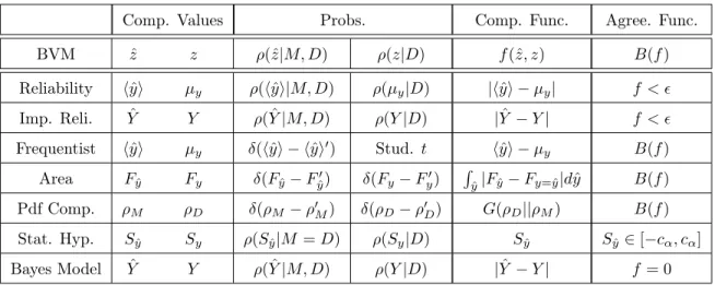
Table 2.1 shows the values of the four BVM inputs that result in the BVM representing the well-known validation metrics as special cases. The following notation is used for the comparison values (^𝑧, 𝑧). The brackets ⟨. . .⟩ denote expectation values, 𝜇’s denote averaged values, ^𝑦, 𝑦 denote single values, ^𝑌 , 𝑌 denote multidimensional values, 𝐹𝑦^, 𝐹𝑦

denote cumulative distribution functions (︀𝐹𝑦 =

∫︀𝑦^

−∞𝜌(^𝑦|𝑀, 𝐷) 𝑑𝑦)︀, 𝑆^𝑦, 𝑆𝑦 denote test

statistics, and [−𝑐𝛼, 𝑐𝛼] denotes the 1 − 𝛼 confidence interval of the data. In the

agreement function column, an element listed as 𝐵(𝑓 ) means the creators of the metric intentionally left the definition of agreement unspecified; however, it is natural to assume it is a function of the comparison function 𝑓 .

(40)

validation metrics as special cases. It also summarizes some of the similarities and difference between the known validation metrics. In particular, by looking at the validation metrics with the same type of comparison values, i.e. the reliability and frequentist or the improved reliability and Bayesian model testing, we can compare them directly. We see that if one lets the frequentist metric allow for more general input probability distributions and the use of a reasonable agreement function (i.e., 𝐵(𝑓 ) is true if |𝑓 | < 𝜖), then the frequentist metric is the reliability metric. Further, in Bayesian model testing, if the agreement function 𝐵(𝑓 ) is loosened to accept 𝑓 < 𝜖, then the pdfs that appear in the Bayesian model testing framework are equal to the improved reliability metric. This information improves the objectivity of the current validation procedure because we now have a map between validation metrics that were originally thought to be different.

Comp. Values Probs. Comp. Func. Agree. Func.

BVM 𝑧^ 𝑧 𝜌(^𝑧|𝑀, 𝐷) 𝜌(𝑧|𝐷) 𝑓 (^𝑧, 𝑧) 𝐵(𝑓 ) Reliability ⟨^𝑦⟩ 𝜇𝑦 𝜌(⟨^𝑦⟩|𝑀, 𝐷) 𝜌(𝜇𝑦|𝐷) |⟨^𝑦⟩ − 𝜇𝑦| 𝑓 < 𝜖 Imp. Reli. 𝑌^ 𝑌 𝜌( ^𝑌 |𝑀, 𝐷) 𝜌(𝑌 |𝐷) | ^𝑌 − 𝑌 | 𝑓 < 𝜖 Frequentist ⟨^𝑦⟩ 𝜇𝑦 𝛿(⟨^𝑦⟩ − ⟨^𝑦⟩′) Stud. 𝑡 ⟨^𝑦⟩ − 𝜇𝑦 𝐵(𝑓 ) Area 𝐹𝑦^ 𝐹𝑦 𝛿(𝐹𝑦^− 𝐹𝑦^′) 𝛿(𝐹𝑦− 𝐹𝑦′) ∫︀ ^ 𝑦|𝐹𝑦^− 𝐹𝑦=^𝑦|𝑑^𝑦 𝐵(𝑓 ) Pdf Comp. 𝜌𝑀 𝜌𝐷 𝛿(𝜌𝑀 − 𝜌′𝑀) 𝛿(𝜌𝐷− 𝜌′𝐷) 𝐺(𝜌𝐷||𝜌𝑀) 𝐵(𝑓 ) Stat. Hyp. 𝑆𝑦^ 𝑆𝑦 𝜌(𝑆𝑦^|𝑀 = 𝐷) 𝜌(𝑆𝑦|𝐷) 𝑆𝑦^ 𝑆𝑦^∈ [−𝑐𝛼, 𝑐𝛼] Bayes Model 𝑌^ 𝑌 𝜌( ^𝑌 |𝑀, 𝐷) 𝜌(𝑌 |𝐷) | ^𝑌 − 𝑌 | 𝑓 = 0

Table 2.1: Specification of the four BVM inputs that give the other validation metrics as special cases. The column headings are the four BVM input val-ues: Comparison Values (^𝑧, 𝑧), Probabilities (𝜌(^^ 𝑧|𝑀, 𝐷), 𝜌(𝑧|𝐷)), Comparison Function 𝑓 = 𝑓 (^𝑧, 𝑧), and the Boolean Agreement Function 𝐵(𝑓 ). The row headings read: Reliability, Improved Reliability, Frequentist, Area, Pdf Compari-son Metrics, Statistical Hypothesis Testing, and Bayesian Model Testing. The denoted data probability for the average in the frequentist metric, Stud. 𝑡, is the Student’s 𝑡-distribution.

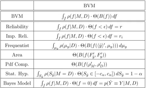
Table 2.2 shows the resulting BVM using the specifications listed in Table 2.1. The value 𝑟 is the standard notation for the reliability metric [47] and we use 𝑟𝑖

(41)

validation metrics as a probability of agreement between the model and the data from Equation (2.2). As no agreement function is specified directly for the frequentist and area metric, the problem is under constrained so the agreement functions are left as general functions over the comparison function 𝐵(𝑓 ). Thus, for any chosen agreement function, the BVM quantifies their probability of agreement. The remaining metrics all do specify (or indicate) an agreement function, and thus, have specified all of the information required to compute the BVM.

BVM BVM ∫︀ 𝑓𝜌(𝑓 |𝑀, 𝐷) · Θ(𝐵(𝑓 )) 𝑑𝑓 Reliability ∫︀_𝑓𝜌(𝑓 |𝑀, 𝐷) · Θ(𝑓 < 𝜖) 𝑑𝑓 = 𝑟 Imp. Reli. ∫︀ 𝑓𝜌(𝑓 |𝑀, 𝐷) · Θ(𝑓 < 𝜖) 𝑑𝑓 = 𝑟𝑖 Frequentist ∫︀ 𝜇𝑦𝜌(𝜇𝑦|𝐷) · Θ(𝐵(𝑓 (⟨^𝑦⟩ ′_{, 𝜇} 𝑦))) 𝑑𝜇𝑦 Area Θ(𝐵(𝑓 (𝐹_^_𝑦′, 𝐹_𝑦′)) Pdf Comp. Θ(𝐵(𝑓 (𝜌′_𝑀, 𝜌′_𝐷)) Stat. Hyp. ∫︀ 𝑆𝑦^𝜌(𝑆𝑦^|𝑀 = 𝐷) · Θ(𝑆𝑦^∈ [−𝑐𝛼, 𝑐𝛼]) 𝑑𝑆𝑦^= 1 − 𝛼 Bayes Model ∫︀_𝑓𝜌(𝑓 |𝑀, 𝐷) · Θ(𝑓 = 0) 𝑑𝑓 = 𝑝( ^𝑌 ≡ 𝑌 |𝑀, 𝐷)

Table 2.2: BVM representation of the other validation metrics as special cases using the comparison functions (the 𝑓 ’s) specified in Table 2.1.

Statistical hypothesis testing is perhaps a bit out of place among the validation metrics. First, note that the comparison function for statistical hypothesis testing is not a function of both the data and the model. Further, note that the model pdf used for statistical hypothesis testing assumes the null hypothesis is true, which in our language is the assumption that 𝜌(𝑆𝑦^|𝑀, 𝐷) = 𝜌(𝑆𝑦^|𝑀 = 𝐷), i.e. that the pdf

of the model is equal to the pdf of the data. This shows how statistical hypothesis testing is a bit out of place here among the validation metrics because here we are attempting to validate a model, usually with its own quantified pdf, rather than, perhaps irresponsibly, assuming it is equal to the data pdf before validating that to be the case. This causes standard statistical hypothesis pitfalls, such as type I (rejecting the null hypothesis when it is true) and type II errors (accepting the null

(42)

hypothesis when it is false), to be carried over into the BVM, which is unwanted. Several comments are made in Appendix A.5 on this issue.

A perhaps surprising result is the proposed functional form of the BVM that rep-resents Bayesian model testing 𝑝(𝐴|𝑀, 𝐷) = 𝑝( ^𝑌 ≡ 𝑌 |𝑀, 𝐷), which is the Bayesian evidence. This is the probability that the uncertain model and data output exactly the same values. Usually what is discussed when reviewing Bayesian model testing is the Bayes posterior odds ratio, i.e. the “Bayes Ratio”,

𝑅 = 𝑝(𝑀 |𝑌 ) 𝑝(𝑀′_{|𝑌 )} ∝

𝑝(𝑌 |𝑀 ) 𝑝(𝑌 |𝑀′₎,

which tests one model 𝑀 (i.e. for validation) against another model 𝑀′. However, in validation metric problems, we are first interested in considering the validation of a single model – the ratio is an extra bit of inference. In Appendix A.6, we show that the BVM result of 𝑝( ^𝑌 ≡ 𝑌 |𝑀, 𝐷) is exactly what we mean by 𝑝(𝑌 |𝑀 ) in the numerator of the Bayes factor,4 which effectively quantifies the validation of a single model against the data 𝑌 , all quantified under uncertainty.

2.5.2 Generalizing the Known Validation Metrics

The BVM offers several avenues to either generalize or improve many of the metrics. The types of generalizations the BVM offer pertain to generalizing the comparison values, comparison functions, definitions of agreement, and/or generalizing deter-ministic comparison values and metrics to the uncertain case. These generalizations are only useful if quantitative statements can be made on their behalf – in such a case, these generalizations are improvements. We will give a brief review of the improvements we found below, but the full discussion is located in Appendix A. By making generalizations or improvements to each of the known validation metrics as implied by the BVM, each metric can be made to satisfy our validation criterion as well as the six desirable validation criteria in [28], due to the results of Section 2.4.

4_{It should be noted that our notation for 𝐷 differs from the notation typically used in Bayesian} model testing. Their 𝐷 is equal to our data 𝑌 , while our 𝐷 refers to context “as having come from the data or experiment rather than the model”.

(43)

Appendix A.1 uses the BVM to show that the reliability metric and the improved reliability metric can be generalized to compare values without a unique order, such as strings, in principle. This involves creating an agreement function over sets of values (such as synonymous sets of strings), rather than continuous intervals, that may be

considered to “agree”.

Appendix A.2 derives the frequentist validation metric and generalizes it to the case where both the model and data expectation values are uncertain. The frequentist metric assumes that the model outputs are known with certainty, which may or may not be true. If a model is stochastic, the model pdfs may be estimated with Monte Carlo or other uncertainty propagation methods that quantify the pdf directly.

Appendix A.3 shows that the area metric may be cast as a special case of the BVM. The area metric involves quantifying the difference between model and data cumulative distributions on a point to point basis; thus, the comparison values (^𝑧, 𝑧) are cumulative distributions themselves. The comparison values are assumed to be known with complete certainty, which in the case of cumulative distributions of data is often difficult to argue. Any quantifiable uncertainty in the cumulative distributions may be integrated over, which generalizes the area metric to situations when the model and/or the data cumulative distributions are uncertain. A drawback is that the BVM in these cases may be very computationally intensive and would likely need to be approximated using a random sampling or discretization scheme. A binned pdf metric is put forward to potentially reduce the computational complexity toward quantifying this generalized area validation metric. This applies similarly to the pdf comparison metrics in Appendix A.4.

In Appendix A.5, we invent an improved statistical hypothesis test using the BVM, called the “statistical power BVM”, that takes into account both model and data pdfs. Because in principle we have a model output pdf 𝜌(^𝑦|𝑀, 𝐷) in model validation problems, we can use it (in place of assuming the null hypothesis is true) to avoid both type I and type II errors.

In the statistical power BVM, the model and the data are defined to agree if both their test statistics lie within one another’s confidence intervals (or “confidence sets” as

(44)

explained in Appendix A.5). The statistical power BVM becomes the product of the statistical powers of the model and data, denoted 𝑝(𝐴|𝑀, 𝐷) =(︀1−𝛽𝑀(𝛼))︀·(︀1−𝛽𝐷( ^𝛼)

)︀ in Equation (A.18). Further comments are made about how systematic error (defined as when a test statistic lies outside of its own confidence interval) may be removed.

It is concluded that the statistical power BVM has a relatively low resolving power compared to other BVMs. This is because large confidence intervals imply large tolerance intervals for acceptance. For this reason, statistical hypothesis testing should only be used for validation in situations where a high degree of nonexactness between model and data test statistics is permissible and the pdfs have very thin tails. This BVM does, however, have a greater resolution than the classical hypothesis test as was proved in Appendix A.5 and will be demonstrated in Section 2.6.

Appendix A.6 finds that Bayesian model testing has the highest possible resolving power because the model and the data are defined to agree only if their values are exactly equal. This is the reverse of what was concluded about statistical hypothesis testing.

Further in Appendix A.6, we argue that, analogous to the Bayesian model testing framework, nothing prevents us from constructing what we call the BVM factor. The BVM factor is,

𝐾(𝐵) = 𝑝(𝐴|𝑀, 𝐷, 𝐵)

𝑝(𝐴|𝑀′_{, 𝐷, 𝐵)}, (2.13)

which is a ratio of the BVMs of two models under arbitrary definitions of agreement 𝐵. Using Bayes’ Theorem, 𝑝(𝑀 |𝐴, 𝐷, 𝐵) = 𝑝(𝐴|𝑀, 𝐷, 𝐵)𝑝(𝑀 |𝐷, 𝐵)/𝑝(𝐴|𝐷, 𝐵), we may further construct the BVM ratio,

𝑅(𝐵) = 𝑝(𝑀 |𝐴, 𝐷, 𝐵) 𝑝(𝑀′_{|𝐴, 𝐷, 𝐵)} = 𝑝(𝐴|𝑀, 𝐷, 𝐵) 𝑝(𝑀 |𝐷, 𝐵) 𝑝(𝐴|𝑀′_{, 𝐷, 𝐵) 𝑝(𝑀}′_{|𝐷, 𝐵)} = 𝐾(𝐵) 𝑝(𝑀 |𝐷, 𝐵) 𝑝(𝑀′_{|𝐷, 𝐵)}, (2.14)

for the purpose of comparative model selection under a general definition of agreement 𝐵. The ratio 𝑝(𝑀 |𝐷, 𝐵)/𝑝(𝑀′|𝐷, 𝐵) is the ratio of prior probabilities of 𝑀 and 𝑀′_.

Analogous to Bayesian model testing, if there is no reason to suspect that one model is a priori more probable than another, one may let 𝑝(𝑀 |𝐷, 𝐵)/𝑝(𝑀′|𝐷, 𝐵) = 1, and

(45)

then 𝑅(𝐵) → 𝐾(𝐵) in value.

Thus, using the BVM ratio, we can perform general model validation testing under arbitrary definitions of agreement and with any reasonable set of comparison functions. The BVM ratio therefore generalizes the Bayesian model testing framework. This will be utilized in Section 2.6.

Finally we wanted to add a note about how one may mitigate the sharpness of the indicator function without using fuzzy logic while also allowing close models to be some-what accepted. As we have seen, it is natural to use a threshold Boolean parameter 𝜖 to help define the boundary of agreement through 𝐵(𝑓 ≤ 𝜖). Such a BVM takes the form,

𝑝(𝐴|𝑀, 𝐷, 𝜖) = ∫︁

𝑓

𝜌(𝑓 |𝑀, 𝐷) · Θ(𝐵(𝑓 ≤ 𝜖)) 𝑑𝑓, (2.15)

where Θ(. . .) instantaneously drops to zero for 𝑓 > 𝜖. One may soften the boundary by allowing 𝜖 itself to be an uncertain quantity, which means one allows their definition of agreement to be somewhat uncertain (which can often be reasonably claimed). As an example, let this uncertainty be 𝜌(𝜖) = 𝜆 exp(−𝜆(𝜖 − 𝜖′)) for 𝜖′ > 𝜖 and zero otherwise, where 𝜆 is positive. Marginalizing over 𝜖 then gives,

𝑝(𝐴|𝑀, 𝐷) = ∫︁ 𝜖 𝑝(𝐴|𝑀, 𝐷, 𝜖) · 𝜌(𝜖) 𝑑𝜖 = ∫︁ 𝑓 𝜌(𝑓 |𝑀, 𝐷) ·(︁Θ(︀𝐵(𝑓 ≤ 𝜖′_{))︀ + Θ(︀𝐵(𝑓 > 𝜖}′_))︀𝑒−𝜆(𝑓 −𝜖′₎)︁ 𝑑𝑓, (2.16) which allows some 𝑓 ’s to be accepted outside the agreement region defined by 𝑓 ≤ 𝜖′, but with an exponentially decaying probability. Other potentially useful 𝜖 pdfs include, but are not limited to: negative slope linear, Gaussian, or decaying sigmoid functions. None of these 𝜖 type distributions were needed to obtain the results of the previous sections explicitly; however, these types of assumptions may have been part of the decision process made implicitly by a practitioner while performing model validation.

(46)

2.6 BVM Examples

In this section, we invent and quantify three novel validation metrics using the BVM to highlight the conceptual clarity, flexibility, and capacity of our framework.

2.6.1 The Statistical Power BVM

Here we consider the statistical power BVM proposed in Appendix A.5 and reviewed in the previous section. This metric defines agreement as occurring when both the model and data comparison values are within one another’s confidence intervals, simultaneously. The BVM for this metric is the product of the statistical powers of the model and the data 𝑝(𝐴|𝑀, 𝐷) =(︀1 − 𝛽𝑀(𝛼))︀ · (︀1 − 𝛽𝐷( ^𝛼))︀, which is calculated in

Equation (A.18). We contrast this with the standard statistical hypothesis test that, after assuming the model is correct, 𝑀 = 𝐷, finds the probability that the model lies within the data’s confidence interval equal to 1 − 𝛼. In statistical hypothesis testing, one then proceeds to check the actual model output and speculates about type I and type II errors. As discussed in Appendix A.5, we do not assume 𝑀 = 𝐷 before validation and therefore type I and type II errors are avoided. Rather, we let the statistical power BVM decide whether or not the model is valid. This provides a more informative validation procedure.

Figure 2-2 depicts a typical statistical hypothesis test scenario that is designed to check the validity of an uncertain model average prediction ^𝜇 (in blue) against an uncertain data average prediction 𝜇 (in red). The data’s 𝜇 is 𝑡-distributed (the same distribution in each subfigure) according to 𝑇 (𝑦, 𝑛 − 1, 𝑠) = 𝑇 (0, 10, 1.75) where (𝑦, 𝑛, 𝑠) are the sample mean, the number of collected data points, and the sample standard deviation, respectively. Each row depicts a normally distributed model centered at 0, but with increasing model variance per row.

The Bayesian validation metric : a framework for probabilistic model calibration and validation

The Bayesian Validation Metric: A Framework for

Probabilistic Model Calibration and Validation

by

Tony Tohme

Submitted to the Center for Computational Science and Engineering

in partial fulfillment of the requirements for the degree of

Master of Science in Computation for Design and Optimization

at the

MASSACHUSETTS INSTITUTE OF TECHNOLOGY

May 2020

c

○ Massachusetts Institute of Technology 2020. All rights reserved.

Author . . . .

Center for Computational Science and Engineering

May 20, 2020

Certified by . . . .

Kamal Youcef-Toumi

Professor of Mechanical Engineering

Thesis Supervisor

Accepted by . . . .

Youssef Marzouk

Associate Professor of Aeronautics and Astronautics

Co-Director, Center for Computational Science and Engineering

The Bayesian Validation Metric: A Framework for

Probabilistic Model Calibration and Validation

by

Tony Tohme

Abstract

Acknowledgments

A Note on the Content

Contents

List of Figures

List of Tables

Chapter 1

Introduction

1.1

Introduction and Overview

1.2

Related Work

1.3

Objectives and Contributions

1.4

Thesis Outline

Chapter 2

The Bayesian Validation Metric

2.1

Introduction

2.2

Notation and Overview

2.3

Formulation of the BVM

2.3.1

Derivation

2.3.2

An Identical Representation

2.3.3

Importance and Statistical Responsibility

2.4

Meeting the Desirable Validation Criterion

2.4.1

Compound Booleans

2.4.2

The BVM Under the Conditions of Exact Agreement

2.4.3

Meeting Underrepresented Validation Criteria

2.5

Representing and Generalizing the Known

Vali-dation Metrics with the BVM

2.5.1

Representing the Known Validation Metrics

2.5.2

Generalizing the Known Validation Metrics

2.6

BVM Examples

2.6.1

The Statistical Power BVM