An arbitrarily high-order, unstructured, free-wake panel solver

An Arbitrarily High-Order, Unstructured,

Free-Wake Panel Solver

by

John Pease Moore IV

OF TECHNOLOGY

NJOV 12 NJ13

UBRARIES

Submitted to the Department of Aeronautics and Astronautics

in partial fulfillment of the requirements for the degree of

Master of Science in Aeronautics and Astronautics

at the

MASSACHUSETTS INSTITUTE OF TECHNOLOGY

September 2013

©

Massachusetts Institute of Technology 2013. All rights reserved.

Author ...

.

..

Iepartment

Certified by ...

H.N. Slater

/

of Aeronautics and Astronautics

August 22, 2013

V 'i

Jaime Peraire

Professor and Department Head

Thesis Supervisor

t

A ccepted by ...

...

Eytan H. Modiano

Profes/or of Aeronautics and Astronautics

An Arbitrarily High-Order, Unstructured, Free-Wake Panel

Solver

by

John Pease Moore IV

Submitted to the Department of Aeronautics and Astronautics on August 22, 2013, in partial fulfillment of the

requirements for the degree of

Master of Science in Aeronautics and Astronautics

Abstract

A high-order panel code capable of solving the potential flow equation about arbitrary

curved geometries is presented. A new method for integrating curved, high-order panels using adaptive Gaussian quadrature is detailed. Furthermore, automated wake handling is addressed and a method to robustly solve for the steady-state free-wake rollup is proposed. Finally, a Fast Multipole Method with a complexity that scales as O(N) is also presented so that large problems can be handled using only a linear mesh. Results are presented to demonstrate high order accuracy and agreement with other inviscid solvers for a variety of test cases.

Thesis Supervisor: Jaime Peraire

Acknowledgments

The author would like to thank the numerous individuals that have made this work possible and have been with me along this journey. First and foremost, I'd like to start by thanking my wife for always being there for me, no matter what. You are so fun to be around, and are always able to put a smile on my face.

I would also like to thank all the students in the ACDL for their support and

company. I have learned a lot from you guys. I would like to thank David Moro for his numerous fruitful conversations about aerodynamics and life in general. Many thanks to Xevi Roca for always being there to answer all my coding inquiries (and, of course, teaching me to surf). I would also like to thank Hemant Chaurasia for always being there to provide advice and encouragement. I would like to thank Ferran Vidal for putting up with me in the office, and for always being there to talk about projects

and have a good laugh.

Additionally, I would like to thank Professor Mark Drela for his numerous advice on boundary element methods and potential flow. It would have been impossible to get to this point without your expertise.

Last, but not least, I would like to thank my advisor Professor Jaime Peraire for his patience, expertise, and wisdom. Even though you are busy with being Department Head, you always make time for your students, and remind us that it is just as important to relax and have a good time as it is to do cool research. All your support and advice is greatly appreciated.

Contents

1 Introduction 13

1.1 Operation Count and Memory Requirements . . . . 14

1.1.1 Mitigation Strategy 1: High-Order Curved Elements . . . . . 14

1.1.2 Mitigation Strategy 2: The Fast Multipole Method . . . . 15

1.2 Approaches to Automated Wake Treatment . . . . 15

1.3 Thesis Contributions . . . . 16

2 Incompressible Potential Flow 19 2.1 Scalar and Vector Potentials . . . . 19

2.2 Boundary Conditions . . . . 20

2.3 Unsteady Bernoulli Equation. . . . . 21

2.4 K utta Condition . . . . 21

3 Discretization ₂₃ 3.1 Boundary Integral Equations. . . . . 23

3.2 Surface Discretization . . . . 26

3.3 Discretization in Time . . . . 27

4 High-Order Element Integration 29 5 Steady-State Solver 33 5.1 The Residual Vector . . . . 33

5.2 T he Jacobian . . . . 34

6 The Fast Multipole Method 37

6.1 Octree Decomposition ... ... 37

6.2 Upward Pass ... ... 38

6.3 Downward Pass . . . . 39

7 Implementation Details and Results 41 7.1 Im plem entation . . . . 41

7.2 High Order Solver . . . . 42

7.3 Steady Solver . . . . 46

7.3.1 Planar Initial Wake and Exact Jacobian . . . . 47

7.3.2 Time-stepped Wake and Approximate Jacobian . . . . 48

7.4 FMM Accelerated BEM . . . . 52

7.4.1 Sphere Convergence Study . . . . 52

7.4.2 Non-lifting Four-Engine Jet . . . . 53

7.4.3 Lifting Business Jet . . . . 54

8 Conclusions and Future Work 59

A Steady-State Jacobian Derivation 61

List of Figures

3-1 Potential shed into the wake in a direction that bisects the trailing edge with a strength equal to the jump in potential between the upper and lower trailing edge surfaces. The wake doublet potential is then converted into discrete vortons which are propagated in time . . . . . 24

4-1 Subdivision of two neighboring elements of order k = 2 showing the subdivided master element (L) and the subdivided source and target elem ents (R ). . . . . 29

6-1 All childless boxes in an octree decomposition about a business jet mesh. 38 6-2 Diagram of FMM translations and interaction lists between two levels

of a 2D grid. Note that the grids on the right and left are identical, and are duplicated for the purpose of visualizing the upward and downward p asses. . . . . 40

7-1 Code fragment taken from the steady-state solver routine. . . . . 42 7-2 Coefficient of pressure for an AR=8 wing with 1652 elements at e = 0

compared to XFOIL using 900 panels. k = 1 solution (L) and k = 3 solution (R ). . . . . 43 7-3 Top view of the Cp distribution at a = 5' computed with the current

BEM solver for k = 3 and the corresponding mesh. . . . . 44 7-4 Coefficient of pressure distribution on an AR = 4 rectangular wing at

a = 5 at the root (L) and 3/4 semispan (R) comparison with FUN3D com puted using k = 1. . . . . 44

7-5 Coefficient of pressure distribution on an AR = 4 rectangular wing at

a = 5 at the root (L) and 3/4 semispan (R) comparison with FUN3D computed using k = 3. . . . . 45

7-6 Lift polar (L) and drag polar (R) for several values of polynomial

ap-proximation k compared to the incompressible Euler solution computed w ith FU N 3D . . . . 46 7-7 Newton solver residual convergence history (L). The unsteady lift

so-lution compared to the steady-state value (R). . . . . 47 7-8 Potential distribution and wake rollup about an AR = 4 swept wing

at a = 5' computed using the nonlinear steady-state code. Front view (L) and top view(R) . . . . 48

7-9 Steady-state Cp distribution and wake roll-up about two second-order wings in tandem computed after 60 time steps . . . . 49

7-10 Steady-state Cp distribution and wake roll-up about a second order

wing and sphere computed after 40 time steps. . . . . 50 7-11 Steady-state Cp distribution and wake roll-up about two Falcon

busi-ness jets flying in tandem computed after 50 time steps . . . . 51 7-12 Potential over a sphere for p = 2 and V, = [1, 0, 0] (L) and error

between the FMM and direct BEM (R). . . . . 53 7-13 Potential solution about four-engine jet (L) and corresponding pressure

distribution (R). Solution time is 240s using multipole expansion order

p= 2 . . . . . . . .. . . 54

7-14 Interpolated pressure coefficient for a business jet operating at a = 5'. 55 7-15 Comparison of the interpolated and non-interpolated pressure

coeffi-cient at a slice plain of Y = 2.5. The distribution on the left is the Cp over the wing, and the distribution on the right is the tail Cp. .... 56

List of Tables

7.1 Convergence of L2 _{norm forr}

Chapter 1

Introduction

Panel methods are currently capable of rapidly solving the potential flow equation on rather complex geometries using only a workstation. These methods, which originated in the early 1960's and are a special case of the Boundary Element Method or BEM, continue to be attractive since the governing equations only need to be solved at the boundary [13, 17, 15, 8]. This eliminates the need for a volume mesh, as is needed when using Finite Difference, Finite Volume, or Finite Element methods, and results in a system which is of comparatively lower dimension. However, there are still two primary open issues in aerodynamic panel methods that this work seeks to address.

The first is that panel methods result in a system of equations that is dense, and memory requirements and matrix assembly complexity grows as the square of the number of degrees of freedom. Additionally, the quantity of interest is usually pressure, which for panel methods is generally obtained by differentiating a piecewise-linear potential field, resulting in only a first-order convergence in pressure compared to the second-order convergence usually obtained with standard CFD solvers. For example, a well-resolved Euler mesh in three dimensions will typically consist of over

100,000 surface elements. If this same mesh and approximation order was used in a

potential flow solver the required memory would be at least 40GB and the pressure would converge at a rate one order lower than the corresponding Euler solution.

The second open issue is treatment of the wake. Vorticity must be shed into the wake in order to produce circulation (and hence, lift) about a lifting body. In practice,

this is usually accomplished by shedding a planar wake extending to infinity from the trailing edge of all lifting surfaces. However, this approach is not physically accurate since the wake should be force-free and convect with the local velocity. Approaches to address these two obstacles are discussed below.

1.1

Operation Count and Memory Requirements

Two methods are proposed for dealing with the dense system of equations that results from the BEM discretization of the potential flow equation. The first is to use high-order curved elements to represent the geometry of interest [25, 26, 29, 6, 161, and the second is to implement the Fast Multipole Method (FMM) and therefore never store the system in memory [12]. These two methods can be used together if desired.

1.1.1

Mitigation Strategy 1: High-Order Curved Elements

Various methods have been proposed to integrate single and double-layer potentials over curved elements including polynomial fitting [26, 29], element subdivision [6], and integrand desingularization through Taylor series expansions [16]. Polynomial fitting approaches are expensive and have only been demonstrated up to second or-der for doublet distributions [26]. Element subdivision approaches have not been capable of accurately computing self-term influences [6]. The integrand desingular-ization approach relies on a B-Spline surface parametrdesingular-ization while also using adaptive quadrature for near-field influences [16]. The integral desingularization approach pre-sented in [16] is difficult to implement and is not extendible to the more general case of NURBS. These high order curved element approaches are particularly attractive for the simulation of rigid geometries since the influence matrix can be computed once and stored in memory for the remainder of the computation.

1.1.2

Mitigation Strategy 2: The Fast Multipole Method

The FMM was developed by Greengard et al. [12] and reduced the computational complexity of performing matrix-vector products in particle simulations from O(N 2₎ to 0(N), with a memory requirement that scales as 0(N log N). In the early 1990's, the FMM was coupled with a Boundary Element Method in order to rapidly simulate circuits [18]. In the late 1990's, this same approach was applied to aerodynamic cases with a computational complexity of O(N log N) [2, 23, 3]. The FMM is attractive for aeroelastic problems where the geometry is deformable since computing a single matrix-vector product with FMM is significantly faster than assembling a new influ-ence matrix at each iteration. The FMM is also useful for large meshes where the system of equations resulting from the BEM discretization is too large to be stored in memory.

1.2

Approaches to Automated Wake Treatment

One of the primary advantages of the BEM is that it has the potential to require minimal pre-processing by the user, in contrast to volumetric methods which may require an experienced user to generate an acceptable volume mesh. However, it is not clear how automatic wake handling for lifting bodies should be treated. There are four popular approaches: (1) fixed-wake, (2) free-wake with panels, (3) free-wake with particles, and (4) vorticity transport. The fixed-wake approach is the simplest and least expensive since it does not involve time marching, but also the least accurate since the fixed wake geometry is somewhat arbitrarily chosen by the user and will vio-late the force-free wake requirement. The second and third approaches are free-wake, meaning that the wake elements or particles travel with the local velocity, satisfying the force-free wake requirement. They are computationally expensive since the only way to robustly obtain the wake position is through time marching. The primary issue with using panels in the wake is that they are singular at their surface. This is problematic if the wake is self-intersecting or intersects the geometry, although an approach using discontinuous basis functions has been proposed to remedy this [27].

Alternatively, vorticity in the wake can be represented with de-singularized vortons at the cost of decreased accuracy. The last approach involves converting the shed vorticity sheet into volumetric vorticity and solving the vorticity transport equation using any of the standard volumetric PDE approaches [4]. However, this requires a well-resolved geometry-conforming volume grid and may be nearly as expensive and require the same amount of pre-processing as solving the full incompressible Euler equations.

1.3

Thesis Contributions

This thesis proposes three approaches to deal with to the aforementioned aerodynamic panel method obstacles:

1. A new algorithm for the integration of arbitrarily high-order single and

double-layer potentials on curved elements using an adaptive quadrature scheme.

2. A new method for solving for the steady-state potential solution and wake roll-up about lifting bodies by casting the BEM and wake evolution equations into

a fully coupled nonlinear system.

3. A Fast Multipole-accelerated BEM with a cost that scales as O(N) compared

to previous potential flow solvers using a similar technique which scaled as

0(N log N) [3, 2] .

The remainder of this thesis is organized as follows. Chapter two will introduce the equations governing incompressible potential flow and the required boundary conditions. Chapter three will detail the discretization in both space and time of the potential flow equation using the BEM. Chapter four will then introduce a new method for integrating the Green's function for Laplace's equation over high-order curved elements. This will be followed by a description of the nonlinear steady-state free-wake solver. Results will then be presented to demonstrate high order convergence, steady-state wake treatment, and application of the solver to complex

geometries. Lastly, conclusions will be drawn and suggestions for further research will be proposed.

Chapter 2

Incompressible Potential Flow

This chapter details the equations governing incompressible potential flow and the necessary boundary conditions. The pressure-velocity relationship governed by Bernoulli's equation and the Kutta condition will also be introduced.

2.1

Scalar and Vector Potentials

Incompressible potential flow can be decomposed into two types of potential: A vector

potential T and a scalar potential

#

can be represented as the superposition of the gradient of the scalar potential, curl of the vector potential, and the freestream velocity:

U=VO+V x X+VOO (2.1)

The continuity equation for an incompressible fluid is

V -U = 0 (2.2)

Equation 2.1 can be substituted into Equation 2.2 to yield Laplace's equation which governs inviscid, incompressible, and irrotational flow

since V - V = 0 and V - (V x IF) 0. The vorticity field, w, is simply the curl of the velocity field:

V x U (2.4)

The evolution of vorticity in time can be derived from the incompressible Euler equa-tion below:

aV U = VpU (2.5)

at p

where p is the pressure and p is the fluid density. The vorticity equation is obtained

by taking the curl of Equation 2.5 and rearranging:

aw

D

= = (W - V) U _(2.6)

at Dt

where 2 denotes the substantial derivative. The right hand side of Equation 2.6_Dt represents vorticity stretching due to the presence of a velocity component in the vorticity direction. Note that this term will vanish in the 2D case since the vorticity vector and stream velocity will always be orthogonal.

2.2

Boundary Conditions

For the case of incompressible potential flow, the correct boundary condition is a no-penetration condition requiring that U -f = 0 on the boundary

U -h = (V#+ V x I + V0) -h = 0 (2.7)

where f is the unit normal vector to the aerodynamic surface. The no-penetration condition can either be enforced explicitly with a Neumann boundary condition on the velocity or implicitly with a Dirichlet boundary condition on the potential inside the body, as will be discussed later.

2.3

Unsteady Bernoulli Equation

Pressure and velocity in an incompressible flow are related through the unsteady Bernoulli equation:

0+ -|IIU112 =|V#+ _{V X Xp+ Vc12_ =-}

(2.8)

at

at

The coefficient of pressure, Cp, is defined as:

CP = (2.9)

Poo

where p,, = !V2 is the freestream dynamic pressure. The coefficient of pressure can be re-written in terms of Equation 2.8 as

a#

1

+- |VO+V x X+Vco0| 2

C2 t 2 2 -1 (2.10)

2.4

Kutta Condition

Inviscid lifting flows require invoking the Kutta condition to enforce pressure conti-nuity at the trailing edge [25]. This work imposes a linearised Kutta condition which requires that the strength of the wake sheet potential 0, must equal the jump in potential from the upper trailing edge surface to the lower trailing edge surface [14]:

0. - 01 =

#W

Note that a nonlinear Kutta condition could be imposed instead, where the pressure at the upper surface of the trailing edge is forced to equal the pressure at the lower surface using a Newton method. A nonlinear Kutta condition is necessary to capture highly unsteady effects, but since this work is primarily concerned with steady-state solutions, it has not yet been implemented.

Chapter 3

Discretization

The potential flow equation is discretized in space using the Boundary Element Method and in time using an explicit Runge-Kutta method. The spatial and temporal discretization schemes implemented in this work are detailed below.

3.1

Boundary Integral Equations

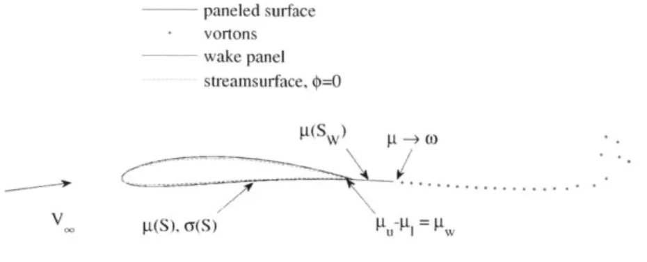
Laplace's equation is discretized using the BEM based on the Morino formulation [17]. Morino's formulation ensures that the perturbation potential is equal to zero inside the aerodynamic body, forcing the surface to become a streamsurface. In practice, this is accomplished by imposing a Dirichlet boundary condition on the perturbation potential an infinitesimal distance inside the surface. A diagram of the surfaces, potentials, and vorton representation used in this work is shown below.

paneled surface - vortons wake panel streamsurface, 0=0 P(S W) t-*o

...

Figure 3-1: Potential shed into the wake in a direction that bisects the trailing edge with a strength equal to the jump in potential between the upper and lower trailing edge surfaces. The wake doublet potential is then converted into discrete vortons which are propagated in time.

The perturbation potential at some point r just inside the aerodynamic body, due to double-layer (doublet) densities distributed over the aerodynamic surface S and wake surface Sw, and the single-layer (source) densities distributed over the aerodynamic surface, is the superposition of the two potentials and must equal zero inside the surface.

q$(r) j (Ga(p, r) + G,(u8(r), r)) + Gd (P, r) = 0 (3.1)

JS JSw

Here Gd is the Green's function for the double-layer potential satisfying Laplace's equation and G, is the corresponding kernel for the single-layer potential. r is the scalar distance between r and a point r, on surface S. The wake surface Sw is required to accurately enforce the Kutta condition. The Green's function for

single-layer potential due to a source of strength a is:

G,(a(r), r) = 1 (r) (3.2)

4-r r

surface normal h, is:

Gd(,ur) 1 & (3.3)

47r Ohs r

The source strength o-, in Equation 3.1 is chosen to equal the component of the wake and freestream velocity influences in Equation 2.1 in the direction normal to the surface:

as(r) (Vo + V(r)) s (3.4)

where the second term is the vector potential velocity contribution from the wake vortons:

Vq,(r) = V x x'(w, r) (3.5)

Here D denotes the entire domain. The vector potential is defined as 1wo

I (w, r) = I + (3.6)

where e is a parameter that removes the vorton singularity and mimics a viscous core. The volume vorticity term o is a function of the shed doublet strength P prescribed by the Kutta condition. Therefore, the only independent variable in Equation 3.1 is the doublet strength p. The conversion of the wake vorticity sheet to volume vorticity is thoroughly detailed in Willis, et al. [7]. Finally, the velocity at any point r given in Equation 2.1 can be written in terms of Equations 3.1, and 3.5 as:

U(r) V(G(P, r)+Gs(u(r),r))+ VGd(P, r)+ jV x (w r)+Voc (3.7)

One of the advantages of the Morino formulation is that the surface doublet den-sity distribution is equal to potential distribution, and surface velocities can be ob-tained by simply differentiating the surface doublet density. Note that the Morino formulation allows the Kutta condition to simply be written as ptu - i = p,.

3.2

Surface Discretization

A Galerkin method is implemented to discretize the Boundary Integral Equations in

space, in a similar approach to the standard Finite Element Method. A Galerkin method was chosen over collocation due to increased accuracy [25]. Let Q be a boundary in 3 composed of S and Th be a collection of elements representing the triangulation of Q. Furthermore, let Q- be the limit of Q as approached from the the interior of the surface S. The Dirichlet boundary condition on the perturbation potential given in Equation 3.1 can now be written in terms of this new notation as:

O(p) = 0 in Q- x (0, T] (3.8)

The following approximation spaces are introduced, which reside in each element K in 7h, and are used to represent the potential solution p and the test function w:

Wh = {w E C0(Q-): W E Pk(K),VK E Th} (3.9)

where Pk(K) is the space of polynomials of degree k which reside in K and C(Q-) denotes the space of piecewise-continuous functions on the boundary Q-. In the current implementation, these polynomials are chosen to be the set of orthonormal Koornwinder polynomials in IZ2. The projection of Equation 3.1 onto a test function

w E W ensures that the solution is orthogonal to the test function:

(OK (P), W) K= 0, Vw G W(K) (3.10)

where, for compactness, the inner product is defined as (a, b)K =K ab. The potential

on each element K in Equation 3.10 is:

OK(P)

I U

where o- (r) is determined from the freestream and wake velocities and also depends on the surface normal h,. Formally, the Galerkin method seeks to find Ph E Wh that

satisfies the projection of Equation 3.8:

(#K (1h), W )Th = 0, Vw C W(Th) (3.12)

which results a system of equations consisting of only the unknown doublet strengths

Ph-3.3

Discretization in Time

One of the advantages of this particular boundary element formulation is that the governing equation (Equation 3.1) does not explicitly include a time-derivative term. This is a result of the fact that the flow is incompressible and that the only condition being enforced is the no-penetration condition on velocity [141. However, there is an implicit dependence on time since the source strength or(r) depends on the wake position and vorticity strength which are permitted to evolve in time. The time-discretization of the governing equation then reduces to the time-time-discretization of the wake only.

The positions of the wake vortons at time t are denoted as x(t) and convect with the local velocity U(x, t) according to the system of ODEs:

dx= U

(3.13)

dt

Similarly, the time-evolution of the vorticity governed by Equation 2.6 is

Dw

D = (o - V)U (3.14)

Dt

The above two equations are integrated in time with a constant time step of At using an explicit Runge-Kutta method with s stages. All results presented in this work were obtained using the 1 stage explicit (Forward Euler) Runge-Kutta method, although any of the implicit or explicit Runge-Kutta methods could be used instead to obtain increased temporal accuracy and stability. The descretization of the wake evolution

using Forward Euler is:

Xfl+l - X

= U(X") (3.15)

At

where the superscript n denotes the time step. Similarly, the discrete vorticity evo-lution equation is:

n+1 _n

Chapter 4

High-Order Element Integration

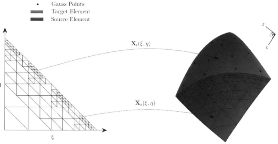
Curved element integration is performed using adaptive Gaussian quadrature. The solution on each element is represented with basis functions which are chosen to be the set of orthonormal Koornwinder polynomials of degree k defined in reference space

- q. The geometry of each element is defined by the mapping X( , ij) from the

reference triangle to the physical element. Two levels of integration are needed. At the innermost level the single and double-layer kernels must be evaluated on each of the elements for each Gauss point used to integrate the test functions. The outer level is the integration over the test functions.

. (auss Points

T argt Element

SSoUrcT Flement z

Figure 4-1: Subdivision of two neighboring elements of order k 2 showing the

Since the self-term integrands are singular and the near-field interactions are close to singular, standard numerical quadrature approaches will fail in these cases. It is easy to compute the rate of integrand decay for both single and double-layer po-tentials, and this rate can be used to create an efficient quadrature algorithm. The following adaptive quadrature scheme is proposed.

for Kt E T do

for xt E Kt do

move target gauss points a small distance r inside surface

for K

C

for x, E K, do

r =

||xt

if fK(r) < C then

Evaluate G.(a, r) and Gd(P, r).

else

Divide K

Compute trial functions on divided K

go to [for x, E K, do] end if

end for

Integrate trial functions over K,

end for end for

Integrate test functions over Kt

end for

where the subscripts s and t denote the "source" and "target" elements and x are the Gauss points belonging to each element K. fK(r) is a distance function which dictates the threshold for which a source element should be divided. In three dimensions the potential due to the single-layer kernel decays at a rate of AKwhile _r the double-layer kernel decays at a rate of (r)AK where AK is the area of element K. A reasonable choice for a cut-off function should satisfy max{ (r-ft)AK AK I C where C is a constant

indicative of the quadrature error committed. In this work, the following threshold function is implemented:

((r

fK(r) = max{ 0 , rr (4.1)

C = 1 and T = 10-10 have proven to be sufficient parameters for the test cases

Chapter 5

Steady-State Solver

In this section, a method is developed to solve the nonlinear free-wake steady-state potential flow problem. The nonlinearity arises from the dependence of the doublet potential on the vorton positions and strengths. Currently, the nonlinear system if solved with the standard Newton method if FMM acceleration is not used. For cases where the FMM method is used to accelerate wake interactions, a Jacobian-free Newton method is used since the resulting analytical Jacobian would be cumbersome to implement.

5.1

The Residual Vector

There are three equations governing the potential flow model detailed above: (1) the condition that the perturbation potential vanishes just inside the body (Equation

3.1), (2) the ODE governing the wake evolution (Equation 3.13), and (3) the ODE

governing the vorticity evolution (Equation 3.14). These equations can be written as a system consisting of the N, surface doublet distribution degrees of freedom, the three components of the NV vorton spatial coordinates, and the three components of the NV vorton vorticity vector. A residual vector written from the three governing equations mentioned above can be defined as:

where 4D is the residual resulting from the Galerkin BEM in Equation 3.12, X is a residual from the Forward Euler discretization of Equation 3.13, and W is the residual from the forward Euler discretization of Equation 3.14. The vorton position residual at time step n is then

X" = x n _ - U(x"-1) - 0 (5.2)

At

Assuming that the wake behavior is non-chaotic, the wake can be forced into lock-step, providing the following relationship:

xj 3 = x _-, j E {Ns + 1, ..., Nv} (5.3)

where Ns is the number of vortons shed at each time step. Since the system is in lock-step, the superscripts can be eliminated from the Forward Euler discretization and the residual vector can be written in terms of the indices xj-N and xj instead. The wake evolution equation can then be re-writen as:

Xi = xj -xj-N - U(xJ-N) = 0, j C {Ns + 1, ... , Nv} (5.4)

The same principal can be used to write a residual vector for the vorticity evolution equation in lock-step:

W3 = Wj - -Nj - (oj -V)U(Xi-N-) = 0, j C {Ns + 1, ..., Nv} (5.5)

A~t

5.2

The Jacobian

The Jacobian of the residual vector with respect to the vector of unknowns u is

where

- -T

U PI1 2 ... /NI X₁ X2 ... XNV W1 W2 ... WNV (5.7)

Differentiating F with respect to u yields the Jacobian matrix

-OCD 04h O<D -& x &w A a JX X =x OX (5.8)

ap

x

and the following system is solved for the update vector 6u at each step of the Newton method until the L2_{-norm of F is sufficiently small.}

Jou = -F (5.9)

The terms of the Jacobian matrix in Equation 5.8 are somewhat tedious to derive and are therefore listed in Appendix A. Additionally, it should be noted that the Jacobian is dense and grows rapidly in size with the number of vortons since there are 6 degrees of freedom associated with each vorton.

5.3

Jacobian-Free Newton Method

The Jacobian-free Newton method is used for cases where the Jacobian cannot be easily computed, as is the case when the Fast Multipole Method is invoked, and where the analytical Jacobian is too large to store in memory. The Jacobian-free Newton method approximates the Jacobian with a finite difference along a search direction. A good search direction is obtained by a Krylov subspace solver. The Jacobian is approximated as:

F(u) - F(u + es) _(5.10)

where s is the direction obtained from driving a Krylov subspace solver residual to a specified tolerance a. c = 10-8 and a = 10-2 have proven to be sufficient for the cases encountered in this work.

Chapter 6

The Fast Multipole Method

This section presents the theory of the Fast Multipole Method and it's application

to the panel method presented in this work. A more detailed description of the

method and associated translation operators can be found in Appendix B. The FMM is composed of three primary routines: the octree domain decomposition, the upward pass, and the downward pass. Each of the three routines are detailed below. Figure

6-2 depicts the primary steps of the FMM algorithm.

The cost of the FMM implemented in this work scales as O(N) were N is the

number of elements in the FEM triangulation. This has a lower cost than previously

implemented aerodynamic FMM-accelerated panel methods such as [25] and [3] which

scaled as 0(N log N). The reduction in operation count compared to these methods

is obtained by implementing the translation operators described below, at the cost of increased implementation complexity.

6.1

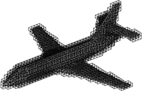
Octree Decomposition

A cubic domain is generated spanning all the sources, doublets, and vortons in space.

The cube is recursively divided into eight boxes, until there are no more than NMAX

elements in a box. Boxes with no elements in them are deleted. The FMM method requires that each cell know who its nearest neighbors and second nearest neighbors are. A nearest neighbor is defined as a box which touches another box, even if they are

just touching at a point. Nearest neighbors can be easily computed by traversing down the octree, searching through the children of each box's parent. The second nearest neighbors can be computed by searching through the nearest neighbors of each box's nearest neighbors. The computational cost of the octree domain decomposition can range from 0(N log N) to 0(N), depending on the homogeneity of the singularity distributions where N is the sum of the number of elements and vortons in the domain.

Figure 6-1: All childless boxes in an octree decomposition about a business jet mesh.

6.2

Upward Pass

The upward pass is composed of two steps: (1) Multipole Generation and (2) the Multipole-to-Multipole (M -+ M) translation. In the Multipole Generation step,

multipole expansion coefficients are computed due to all sources, dipoles, and vortons in each childless box. This will result in five expansion coefficients for each box, corresponding to the source distribution, doublet distribution, and three components of vorticity due to the vortons. The complexity of this step is O(Np2_{), where p} is the order of the multipole expansion. The Multipole-to-Multipole translation is the recursive translation of the multipole coefficients up the tree, starting with the childless boxes. The computational complexity of this step is O(Np4_).

6.3

Downward Pass

The downward pass is composed of four steps: (1) the Multipole to Local (M - L)

translation,(2) the Local to Local translation (L -+ L), (3) the Direct Evaluation, and

(4) the Local Expansion evaluation. The (M -± L) translation involves the conversion

of all the multipole expansions of the boxes in a box's interaction list into a Taylor series expansion about the box's center. The interaction list can be chosen to be all

the second nearest neighbors of a box, or a more complicated criteria [12]. This is

the most expensive part of the FMM algorithm due the large number of boxes in the second nearest neighbor list and since this operation has a complexity that scales as

O(Np4). The L -+ L translation is a recursive translation of local coefficients down

the octree from each box to it's child. The complexity of this operation scales as

O(Np4_{). The Direct Evaluation step computes the interaction between all sources,}

dipoles, and vortons in a box and that box's nearest neighbors directly without using multipole expansions. The complexity of this operation is O(Ns), where s is a measure of the cost required to analytically integrate the source and dipole distribution over a element. The final step is the evaluation of the Local Expansions in each childless

box. This step has a complexity of O(Np2₎

since it is not a translation operation, only a local evaluation.

Source Box

Zi| Interaction List Nearest Neighbors

T-rget Box Parent of Source

- Parent of arget _{-Al - L}

Upward Pass

Downard Pass

I~b

Figure 6-2: Diagram of FMM translations and interaction lists between two levels of a 2D grid. Note that the grids on the right and left are identical, and are duplicated for the purpose of visualizing the upward and downward passes.

-Chapter 7

Implementation Details and

Results

This section discusses implementation and presents results including demonstration of high-order convergence, validation of the nonlinear steady-state solver, and the extension of Fast Multipole accelerated BEM to large problems.

7.1

Implementation

The high order solver is written in C++ and heavily relies on the Armadillo C++ linear algebra library [21] which provides an intuitive syntax and simple access to

BLAS routines which are typically cumbersome to invoke. The Armadillo library is

linked to Intel's Math Kernel Library for best performance. Additionally, the matrix assembly routine is parallelized with OpcnMP to reduce runtimes. Armadillo provides a simple, MATLAB-like syntax that allows for easy prototyping. An example of a code fragment written in Armadillo is shown below:

timer.tic();

state.mu = solve(pmats.d,-pmats.s*sigma);I

cout << "solution time: " << timer.toc() << endl; // Compute the potential gradient

mat gradsol = solutiongradient(master, mesh.elementsmesh.nodes, state.mu);

Figure 7-1: Code fragment taken from the steady-state solver routine.

7.2

High Order Solver

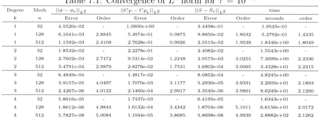
Convergence results for the potential flow around the unit sphere are presented using increasing orders of polynomial approximation k. The analytical solution is known, and the polynomial degree is increased from k = 1 to k = 4 while uniformly refining the mesh from n = 32 to n = 512 elements. The meshes were generated using the open-source mesh generation software GMSH [5, 1]. All errors are computed in the

L2- norm.

I -O

a Ue i.1: Convergence Ut L- norm torT = IU

Degree Mesh ||0 - 0e|HL2 ||Cp - CPe 1IL2 HIS - Se| L2 time

k n Error Order Error Order Error Order seconds order

32 128 512 32 128 512 32 128 512 32 128 512 4.5520e-02 6.1641e-03 1. 1592e-03 1.8532e-02 2.7602e-03 3.4791e-04 6.4849e-04 3.9157e-05 2.4267e-06 5.8916e-05 1.8612e-06 5.7827e-08 2.8845 2.4108 2.7472 2.9879 4.0497 4.0122 4.9844 5.0084 1.0900e+00 5.4974e-01 2.7628e-01 2.2278e-01 9.5314e-02 2.8276e-02 1.4817e-02 1.7070e-03 2.1460e-04 1.7437e-03 1.6132e-04 1. 1044e-05 0.9875 0.9926 1.2248 1.7531 3.1177 2.9917 3.4342 3.8685 3.4498e-01 9.8850e-02 2.5515e-02 2.4082e-02 2.9575e-03 3.6802e-04 8.0852e-04 5.2930e-05 3.3540e-06 6.4195e-05 1.8704e-06 5.8698e-08 1.8032 1.9539 3.0255 3.0065 3.9331 3.9801 5.1011 4.9939 1.9545e-01 5.2792e-01 1.8446e+00 1.5543e+00 7.3099e+00 3.4328e+01 4.8245e+00 2.2005e+01 9.6249e+01 1.6343e+01 6.6156e+01 2.8882e±02 1.4335 1.8049 2.2336 2.2315 2.1893 2.1290 2.0172 2.1262

Table 1 shows that the potential converges at the optimal rate of k

+

coefficient of pressure only converges with rate k. This loss of an order is expected as the coefficient of pressure is obtained by differentiation of the surface potential. Additionally, the geometry converges with

computational time grows approximately linearly with the number of elements, since

the optimal rate of k

+

quadratically with the element size and the cost of computing self-term influences

is far greater than computing far-field terms.

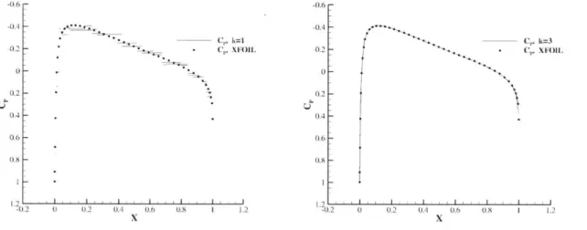
In order to test a slightly more challenging case the pressure coefficient about a finite aspect ratio wing at a = 0 is compared to a well-resolved XFOIL

[9]

-0.6 -0.6 --0.4 - c~ -0.4 -0.2 - C1, XFOIL 0.2

{

Figure 7-2: Coefficient of pressure for an AR=8 wing with 1652 elements at a 0

compared to XFOIL using 900 panels. k = 1 solution (L) and k = 3 solution (R).

It is clear that a significant error is committed in the coefficient of pressure for the standard linear (k = 1) panel method since the pressure is piecewise-constant on

each element. However, the pressure distribution computed with k = 3 lies on top of the XFOIL solution, indicating that a third-order solution using the current mesh is k-converged.

Finally, results for the case of a lifting wing of aspect ratio 4 with a NACA0012 airfoil section are presented and compared to second-order-accurate incompressible

Euler solutions computed with FUN3D [11]. A low aspect ratio was chosen in order to test the ability of the current method to capture moderate 3D effects. The surface mesh specifications are identical to the non-lifting case presented above, except for the fact that the aspect ratio is now 4 instead of 8. For this case, a fixed, planar wake consisting of 20 stream-wise elements extending 103 chord lengths downstream is implemented. The FUN3D mesh consists of 4.1 million tetrahedral elements, with the wing boundary being composed of 221,862 triangular elements. The leading and trailing edge spacing for the FUN3D mesh is c . 10-3 where c is the chord length.

1.

-0.5

-1

Figure 7-3: Top view of the Cp distribution at a = 5' computed with BEM solver for k = 3 and the corresponding mesh.

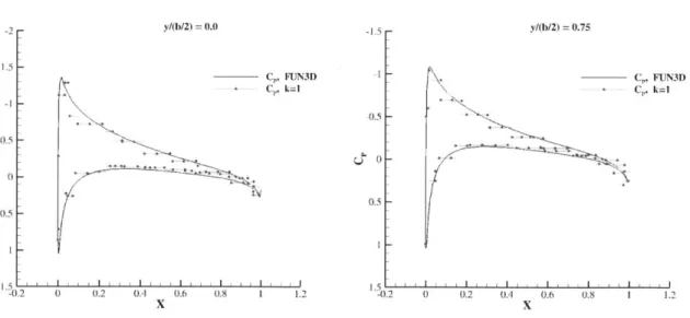
the current y/(b/2) = 0.0 _-1.5 -I1 C,, FUN3D C, k=1 0.5 0 0.5 1 1.2 .5 0 0.2 04 0.6 0.8 x

Figure 7-4: Coefficient of pressure distribution on an AR = 4 rectangular wing at a = 5 at the root (L) and 3/4 semispan (R) comparison with FUN3D computed using k = 1. -2 -1.5 -1 -0.5 0 0.5 y/(b/2) = 0.75 C, FUN3D C,. k=1 0.2 0 0.2 0.4 0.6 0.8 x 1 1.2 i ; i i I i I i . 2

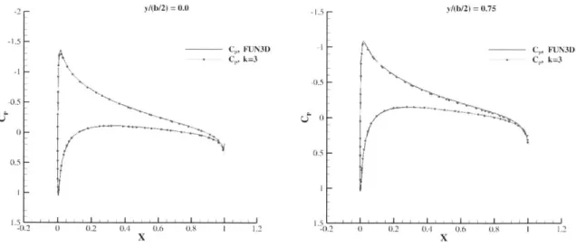
y/(b/2) = 0.0 C, FUN C, k=3 -1.5 -0.5 0.2 1.5 3D -0,5 0. 5 V-12 2 I I I I I III . I I 1) 0.2 04 0.6 0.8 X

Figure 7-5: Coefficient of pressure distribution a = 50 at the root (L) and 3/4 semispan (R) using k = 3.

on an AR = 4 rectangular wing at comparison with FUN3D computed

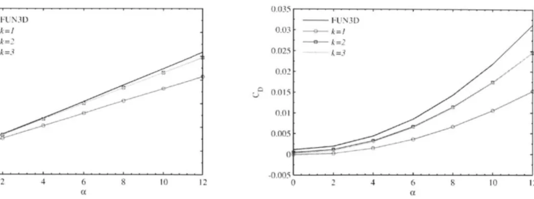
Figures 7-4 and 7-5 show the pressure distributions at two slice locations along the span, b, computed using k = 1 and k = 3, respectively. It can be observed that there is a significant error in the pressure distribution for the k = 1 case at both span-wise locations, but this error is significantly reduced by using a high polynomial degree. The pressure computed using k = 3 lies on top of the FUN3D solution at the wing root, and there is only a slight over-prediction of the upper surface pressure at 3/4 semi-span when compared to FUN3D. Note that a difference between the FUN3D solution and the current method should be expected since the results presented above are computed using a fixed planar wake which violates the force-free wake requirement. An angle of attack sweep is conducted in order to validate accuracy over a range of conditions. The angle of attack is increased from 0 to 12 degrees in two degree increments for k =

{1,

0 0.2 0.4 0.6 08 X C, FUN3D C, k=3 I I I I I I I 1.2 y/(b/2) = 0.75

FUN3D -FUIN3D 0.5 -e k =I 0.03 - - -k =I --= k=2 0.4 k=3 0.025 3 0.3 0.015 0 0

Figure 7-6: Lift polar (L) and drag polar (R) for several values of polynomial approx-imation k compared to the incompressible Euler solution computed with FUN3D.

The lift and drag computed with k = 1 differ significantly from the results obtained with FUN3D and higher order polynomial approximations. This indicates that for the current mesh, the solution is not k-converged with k 1. The solutions computed

with k = 2 and k = 3 are almost identical. For k 3 the lift differs from the

Euler solution by approximately 5% while the drag differs by 17% at a = 12'.The discrepancy between the polars computed using the high order BEM and the Euler case is likely a result of using a fixed wake in place of the more expensive but also more accurate free wake. Although the drag computed with the potential solver differs from the Euler values, it exhibit the correct trend and grows with the square of the angle of attack. Note that the drag at a = 0 obtained with FUN3D is not zero as it should be, and the k = 2 and k = 3 BEM solutions appear to be better at

predicting zero lift at zero angle of attack.

7.3

Steady Solver

Two methods for obtaining a steady-state solution are presented. In the first, the wake is seeded with vortons extending in a plane from the trailing edge. A Newton solver is then invoked and the residual is driven to zero. However, this initial condition may not be sufficient for cases where the wake strongly interacts with bodies downstream. Therefore, a second method is presented whereby the wake is time-stepped for a

prescribed number of steps, and then the nonlinear steady-state solver is invoked. Additionally, either an exact or approximate Jacobian may be used depending on whether or not FMM acceleration is enabled.

7.3.1

Planar Initial Wake and Exact Jacobian

An AR = 4 swept wing with a leading edge sweep angle of A = 150 and taper ratio of A = 0.8 composed of 996 linear elements is used to validate the steady state solver against an unsteady solution. The wake is seeded with 100 lock-steps of vortons spaced I VI| At = 0.2 apart. A Newton solver with line search is used to drive the norm of the residual to a small tolerance, chosen to be 10-10. Preconditioned GMRES

[20] is used for the linear solve since it was found to be faster than a direct solver. GMRES without preconditioning is significantly slower than using a direct solver since the condition number of the system is generally between O(10') and O(10')

(it was later discovered that the condition number could be substantially reduced by re-ordering the wake degrees of freedom). The LU decomposition of the Jacobian computed during the first Newton iteration is used as the preconditioner for the remainder of the Newton iterations. The steady-state solution and lift comparison with the unsteady solver are shown below.

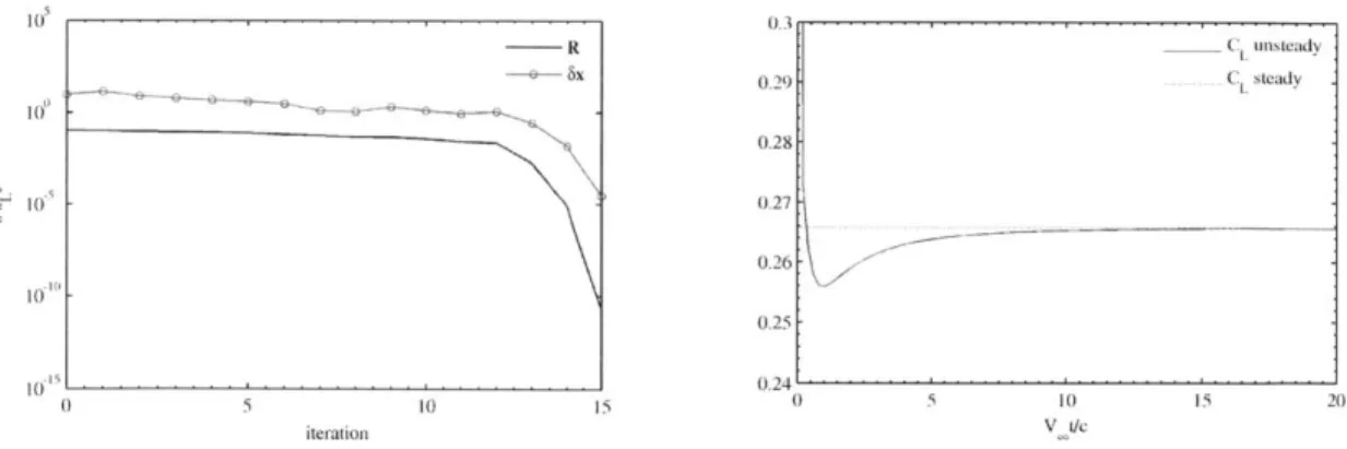
10 0.3 - -R C unsteady 0.29 t L~d 0.28-10 0.27 0.26 10 0.25 _______0________________________ 0.24 ...---0 10 1.4 5 1' 5 20 iteration V t/c

Figure 7-7: Newton solver residual convergence history (L). The unsteady lift solution compared to the steady-state value (R).

Figure 7-8: Potential distribution and wake rollup about an AR 4 swept wing at

OZ = 5' computed using the nonlinear steady-state code. Front view (L) and top

view(R)

After Voet/c = _{20, the unsteady CL is within 0.05% of the steady-state value,} indicating that the unsteady solution is converging to the steady-state result. Figure

7-7 shows that the Newton solver only requires 15 iterations to converge to a tolerance

of 10-10. The solution time required for the case above was 865 seconds, 10 of which were spent computing the preconditioner and 3 of which were spent solving the linear systems with GMRES. The remainder of the time was spent in the Jacobian

assem-bly routine, since the Jacobian must be completely re-assembled for each Newton

iteration. 441MB of memory was required to store the dense Jacobian matrix.

7.3.2

Time-stepped Wake and Approximate Jacobian

Three cases are presented to demonstrate the robustness of the steady state solver. The first is for two second-order accurate wings of the same geometry as described in the previous section flying in tandem. The wings are separated by a distance of three root chord lengths. The second case is for the same second-order wing but with a sphere located at a distance of five root chord lengths downstream instead of a second wing. The last case is that of two first-order accurate Falcon business jets flying in tandem at an (unrealistically) close distance.

... ... ... ... ... ... ... ... . ... . ... 4 ... ... ... ... tv"% ... ... ... ... ... *.t. ... %'13 *419 ... ... ... ... ... ... ... .... ;-4 a) 7: 7 C) A-D C) UO CY) C) LO C\j 4-D C; I 4-D Ln r-co Q0 4--) C; 7 LO C C) 4-D 4-D 4-D DO 7 4-D bjO bjO

-1.25 -0.6875 -0.125 0.4375

Figure 7-10: Steady-state Cp distribution and wake roll-up about a second order wing and sphere computed after 40 time steps.

IL

.*g. **.. L .~%A~* tt.* *1~ .4- * * ~ . -1.25 -0.6875 -0.125 0.4375 1

Figure 7-11: Steady-state Cp distribution and wake roll-up about two Falcon business jets flying in tandem computed after 50 time steps.

The above three cases demonstrate the robustness of the current wake model. For each of these cases, the wake is evolved for a specified number of time steps, after which the nonlinear fully-coupled solver is turned on. For the two-wing test case, the wake of the front wing travels over the aft wing, and interacts with the aft wing's wake. The wake shed from the wing in the wing-sphere case travels around the sphere as expected. Note that this case would be impossible to evaluate if linear panels were used to represent wake vorticity since the singular wake panels would intersect the sphere. The two-jet case demonstrates that the wake model is readily extendible to complex geometries, and the wake of the fore wing can be observed interacting with the second jet's surface and wake.

7.4

FMM Accelerated BEM

This section presents results for three cases of increasing complexity. The first is for flow about the unit sphere in order to demonstrate FMM convergence. The second is for non-lifting flow about a four-engine jet aircraft. The third is the case of a lifting business jet with a fixed wake.

Although the cases presented below all use linear meshes, the FMM is readably extendible to high order meshes as well. Solutions have been computed using the FMM-accelerated BEM with high-order meshes using the current solver. However, in the current implementation there is no benefit to coupling the two methods since the high-order integration techniques already scale as O(N) due to the rate-limiting self-term influence integral. If a more efficient method for computing self-self-term integrals for high-order elements is developed in the future, then the benefits of both high order accuracy and the reduced FMM operation count could be realized at a fraction of the cost of the current high-order solver.

7.4.1

Sphere Convergence Study

The case of a unit sphere represented with 855 linear elements is chosen to demon-strate the convergence of the FMM method in multipole expansion order p. The error is quantified by computing the L2-norm of the difference between the FMM solution and the solution generated with the direct BEM solver. Both the FMM and BEM system of equations are solved with GMRES to machine precision, and the only dif-ference is in the approximate matrix-vector product of the FMM compared to the machine precision matrix-vector product of the direct BEM solver.

0.5 0.5 010 --0.5 10" 1 2 3 4 5 6 7 8 9 10

Figure 7-12: Potential over a sphere for p 2 and V,= [1, 0, 0] (L) and error between the FMM and direct BEM (R).

Even with p = 2, the error in potential is small, however the error in pressure is more significant. This is due to the fact that the velocities are obtained by dif-ferentiation of the potential field, leading to a reduction in pressure accuracy. If a higher pressure accuracy is needed, the multipole order can be increased to obtain the desired fidelity. Note that the errors do not decay very fast in p. Therefore, if a high accuracy is desired then a sufficiently large value of p must be chosen. This can become expensive since the cost of the FMM presented in this work grows as

O(np

7.4.2

Non-lifting Four-Engine Jet

In order to test a more complicated case, a four-engine jet represented with 175,712 linear elements is simulated using the FMM with a multipole expansion of order

p = 2. The mesh was generated with the SUMO [22] mesh generator. This case does

not include a wake influence, and is therefore non-lifting. The near-field interactions are computed directly, and stored in the box data structure once at the beginning of the simulation for efficiency. Additionally, a preconditioner is implemented in order to reduce the number of Krylov subspace iterations required.

Since the FMM provides a method of de-coupling near field and far-field terms, it also provides a very straightforward framework for generating a preconditioner. The preconditioner is applied in a box-by-box manner. For each childless box, the direct

influence matrix is assembled into a square matrix based on the Galerkin discretiza-tion. The resulting matrix is then inverted and stored in memory for the remainder of the computation. The FMM matrix-vector product is computed first, and the preconditioner is applied to the result by looping through the list of childless boxes.

C 0.5 0.5 0 -0.5 -0.5

Figure 7-13: Potential solution about four-engine jet (L) and corresponding pressure distribution (R). Solution time is 240s using multipole expansion order p = 2.

A total of 39 GMRES iterations were required to reach a residual tolerance of 10-6. The solution time for this rather complicated test case was 240 seconds using four processors. The memory required to store the preconditioner was 141MB, and the memory required to store the multipole coefficients and octree structure was 278MB.

If this case were to be solved with the standard dense BEM, 62GB of memory would

be required.

7.4.3

Lifting Business Jet

Lastly, case of lifting potential flow about a fine business jet mesh is demonstrated.

A fixed panelled wake is implemented, extending to infinity. Since the wake extends

to infinity, the octree decomposition of the domain required by the FMM cannot be generated. Therefore, the wake influence is computed directly. Note that this should not be problematic, since the wake influence matrix is much smaller than the full aerodynamic influence matrix would be. The mesh was generated in GMSH and consists of 31,398 linear elements. The process of generating the mesh from a .stp file was essentially hands-free, and only required specifying one parameter controlling