Dynamic soaring beyond biomimetics: control of an albatross-inspired wind-powered system

(1)

Dynamic soaring beyond biomimetics:

control of an albatross-inspired wind-powered system

by

Gabriel D. Bousquet

B.S.,

Ecole

Normale Superieure and Univ. Pierre et

MAOTECHN OLO Y

FEB 09

2018

LIBRARIES

Marie Curie (2007)

S.M., Ecole Normale Superieure and Universite Paris-Sud (2009)

S.M., Ecole Normale Superieure and Universit6 Paris-Diderot (2010)

Submitted to the Department of Mechanical Engineering

in partial fulfillment of the requirements for the degree of

Doctor of Philosophy in Mechanical and Ocean Engineering

at the

MASSACHUSETTS INSTITUTE OF TECHNOLOGY

Februray 2018

@

Massachusetts Institute of Technology 2018.

Author ...

Certified by..

All rights reserved.

Signature redacted

_...

Department of Mechanical Engineering

Noverner 6, 2017

Signature redacted

Jean-Jacques E. Slotine

Professor of mechanical engineering and information sciences and of

brain and cognitive sciences

Thesis Supervisor

Accepted by .

...

Signature redacted

Rohan Abeyaratne, Quentin Berg Professor of Mechanics

Chairman, Department Committee on Graduate Theses

(2)

Dynamic soaring beyond biomimetics: design and control of

an albatross-inspired wind-powered system

by

Gabriel D. Bousquet

Submitted to the Department of Mechanical Engineering on November 6, 2017, in partial fulfillment of the

requirements for the degree of

Doctor of Philosophy in Mechanical and Ocean Engineering

Abstract

Albatrosses extract their propulsive energy from horizontal winds in a maneuver called dynamic soaring, and travel impressive distance (5000 km/week) by "riding the winds". Accordingly, for albatrosses flight is barely more strenuous than rest. While thermal soaring, exploited by birds of prey and sports gliders, consists of simply remaining in updrafts, extracting energy from horizontal winds necessitates redistributing mo-mentum across the wind shear layer, by means of an intricate and dynamic flight manoeuver.

Historically, dynamic soaring has been described as a sequence of half-turns con-necting upwind climbs and downwind dives through the surface shear layer. Re-laxing the half-turn hypothesis, this thesis numerically and analytically studies the "minimum-wind" problem i. e. the question of how much wind is required to stay aloft with dynamic soaring, and what is the optimal flight strategy to do so. Contrary to current thinking, but consistent with GPS recordings of albatrosses, it is shown that when the shear layer is thin the optimal trajectory is composed of small-angle, large-radius arcs. Essentially, the albatross is a flying sailboat, sequentially acting as sail and keel, and most efficient when remaining crosswind at all times. The thin-shear analysis is then extended asymptotically, predicting in closed-form the most efficient dynamic soaring trajectory in wind shears of finite thickness.

Building upon the conceptual study of dynamic soaring, a robotic system inspired

by the albatross is proposed: the "flying sailboat", i. e. a low-flying, water-skimming airplane powered by a keel-and-sail combination. Potentially, the flying sailboat could travel 10x faster than a traditional sailboat of the same size, survive in much rougher seas than hydrofoil boats, and carry 10x more payload than a naive robotic copy of the albatross. A mechanical prototype is presented, with the keel and height controlled with feedback-linearization controllers. Experimental results demonstrating the crit-ical aspects of the system's operation and control are reported: stable extreme-low height flight concurrent with controlled keel immersion and force generation.

(3)

Thesis Supervisor: Jean-Jacques E. Slotine

Title: Professor of mechanical engineering and information sciences and of brain and cognitive sciences

(4)

Acknowledgments

I want to acknowledge first and foremost my advisor Professor Jean-Jacques Slotine

for his mentorship, guidance and support, and many eye-opening insights over the years. I would like to acknowledge my thesis committee members who have all been decisive. Specifically, I want to thank Professor Mark Drela for his pivotal advice in all aerodynamic and experimental matters, Professor Alex Slocum for inspiringly communicating his drive and support, Professor Michael Triantafyllou for his guidance and for inspiring me with smart flight and dynamic soaring.

I would like to acknowledge my labmates and all members of 5-423 and friends,

especially Amy, Audren, Jacob, James, Jodo, and Leah for their friendship, and sharing the ups and downs of navigating graduate school.

My thesis would have remained a thought experiment without the critical help

of Mark Belanger, Dave Lewis and the EDS lab, the warm welcoming, help and friendship of the LAMSS while I was carrying experiments on the Charles River, specifically Mike Benjamin and Misha Novitzky, as well as the help from the sailing pavilion team, particularly Stew Craig.

I am grateful to my friends worldwide, from Boston to London to Princeton to the Bay and elsewhere-you know who you are.

I acknowledge my sponsors over the years. They all brought me much more

than financial support. Fulbright made me discover a precious network of worldwide inspirational colleagues become friends, in particular Arturo, Dovan, Eduardo, Emily, Heather, Kirt, Robbie, and Ronan. The Amar G. Bose research grant provided me with the opportunity to explore and create beyond my initial expertize. SMART was an extremely valuable experience. The Link foundation fellowship proved pivotal as it enabled the experimental aspects of this thesis. Finally, my TAs for 2.017, 2.151,

2.152 and 2.154 introduced me to the enjoyment of communicating knowledge, and

brought me new friends, as well as the pleasure to work with Franz Hover.

Above all, I want to thank my partner Axum for her support, and for the privilege of looking up to her by her side every day.

(5)

I

Dynamic soaring analysis

soaring

2 Optimal dynamic soaring consists of successive shallow arcs 2.1 Introduction . . . . 2.2 M ethods . . . . 2.2.1 Wind model . . . . 2.2.2 Equations of motion . . . .

2.2.3 Non-dimensionalisation . . . . 2.2.4 Numerical trajectory optimization . . . .

2.2.5 Dimensions for the wandering albatross' flight . . . . .

2.2.6 Crosswind flight of the wandering albatross . . . .

2.3 R esults . . . . 21 . 21 . 21 . 22 . 23 . 25 . 29 . 31 . 32

34

35 35 37 37 40 41 42 45 47 51

(6)

2.3.1 Three-dimensional minimum-wind trajectories in a logistic wind p rofile . . . .

2.3.2 Analytic solution in the thin shear layer regime . . . . 2.4 Tlreatment with explicit residuals . . . . 2.4.1 Comparison with recordings of wandering albatrosses and other

numerical studies .

2.5 D iscussion . . . .

2.6 Conclusions . . . . 3 Dynamic Soaring in Finite-Thickness Wind Shears:

Solution

3.1 Introduction . . . .

3.2 M odeling . . . .

3.2.1 Hybrid system . . . .

3.2.2 Airspeed gains and losses during transition . .

3.2.3 Climb and heading angles . . . . 3.2.4 Planar motion . . . .

3.3 Problem formulation and solution . . . . 3.4 Validation and discussion . . . .

63 68 an Asymptotic 79 . . . . 79 . . . . 80 . . . . 81 . . . . 81 . . . . 82 . . . . 83 . . . . 84 . . . . 86

3.4.1 Validation against numerical trajectory optimization in a

logis-tic w ind profile . . . .

3.4.2 Validation against trajectory optimizations in logarithmic and

power-law wind profiles . . . .

3.4.3 Validation against recordings of flying albatrosses . . . .

3.5 Conclusions . . . ..

II A biologically-inspired, wind-powered, air/water

cle

86 87 92 92

vehi-94

4 Control of a flexible, surface-piercing hydrofoil for high-speed,

small-scale applications 95

51 53 57

(7)

4.1 Introduction . . . . 96

4.2 Experimental setup . . . . 99

4.2.1 Hydrofoil system . . . . 99

4.2.2 Test rig . . . . 101

4.3 Modelization and parameterization . . . . 102

4.3.1 Sea state and hydrodynamic relative velocities . . . . 103

4.3.2 Added mass . . . . 103

4.3.3 L ift . . . . 104

4.3.4 Other hydrodynamic forces . . . . 105

4.3.5 Dynamics . . . . 105

4.4 C ontrol . . . . 107

4.4.1 Control objectives . . . . 107

4.4.2 Simplified foil equations for control . . . . 107

4.4.3 Controller . . . . 108

4.4.4 Hydrofoil immersion and retraction . . . . 109

4.5 Experimental Results . . . . 110

4.6 Conclusions . . . . 111

5 Wind-powered, airborne oceanic vehicles: from the albatross to the flying sailboat 114 5.1 Introduction . . . . 114

5.2 Albatrosses and sailboats: a functional description . . . . 116

5.2.1 The albatross: Low wind-energy extraction efficiency but large lift-to-drag-ratio, good seakeeping properties enabled by weak coupling . . . . 116

5.2.2 Displacement sailboats: efficient wind extraction with a large drag . . . . 118

5.2.3 Hydrofoil sailboats: efficient wind extraction and high perfor-mance, but at a price in seakeeping . . . . 119

(8)

5.4 From the albatross to the amphibious dynamic soaring the flying sailboat: a continuum of designs . . . .

5.4.1 The amphibious dynamic soaring glider . . . . . 5.4.2 The dihedral flying sailboat . . . . 5.4.3 The flying sailboat . . . . 5.4.4 Other designs . . . . 5.5 Conclusions . . . . glider and to . . . . 122 . . . . 122 . . . . 124 . . . . 126 . . . . 128 . . . . 130

6 The flying sailboat-design and control 6.1 Introduction . . . . 6.2 flying sailboat: a high-speed, wind-powered, air-water system for ocean . . . . 13 4 6.3 Performance analysis . . . . 6.3.1 Trim analysis . . . . 6.3.2 Performance . . . . 6.3.3 . An operational challenge: keel 6.4 Critical maneuver . . . . 6.5 Control . . . . 6.5.1 Longitudinal control . . . . . 6.5.2 Roll control . . . . 6.5.3 Yaw control . . . . 6.5.4 Keel control . . . . 6.6 Experiment . . . . 6.6.1 Experimental setup . . . . 6.6.2 Flight sequence . . . . 6.7 Experimental Results . . . . . . . . 135 . . . . 136 . . . . 138

size and force . . . . 141

. . . . 142 . . . . 143 . . . . 143 . . . . 145 . . . . 146 . . . . 146 . . . . 147 . . . . 147 . . . . 148 . . . . 148

6.8 Simulation of the longitudinal control in the presence of model uncer-tainty, waves, and unmeasured wind gusts . . . .

6.9 C onclusions . . . . monitoring 131 131 150 158

(9)

III Conclusions ₁₅₉

7 Conclusions ₁₆₀

7.1 Thesis contributions ... . 160 7.2 _{Future work . . . 161}

(10)

List of Figures

1-1 Total number of months with f C02 values per 1 x1* grid cell for 1970 through 2014 in SOCAT version 3, from [I]. . . . . 23

1-2 Ocean monitoring systems . . . . 24

1-3 Array of drifters and floats in the Global Drifter and Argo programs. 26

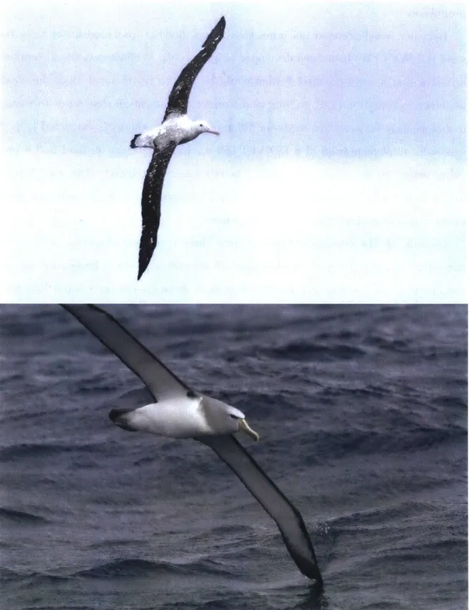
1-4 Wind power energetics. Albatross credits: Raja Stephenson. . . . . . 27 1-5 Albatross in flight Top: Wandering. Bottom: Salvin's (unverified).

Credits: Raja Stephenson. . . . . 30 1-6 Global distribution of some albatrosses species. Source:

[2]

. . . . 31 2-1 Wind profile. (a) Wind field behind waves. Color-coding: wind

intensity. Experimental data adapted from [3]. (b) The logistic wind profile in this study captures adequately the wind field in separated regions, such as behind ocean waves. More generally, it constitutes a robust way to approximate a wide class of wind fields, based on two parameters: a typical wind speed inhomogeneity Wo separated by a shear layer of typical length-scale 6. (c) Rayleigh's wind model is the limit of the logistic profile for 6 -+ 0. . . . . 38

(11)

2-2 The albatross' trajectory. (a) Recording of a flying albatross from

[I

(top view). In crosswind flight the typical turn of the albatross is about

50-700. Dot-dashed yellow portions of the trajectory: the albatross is involved in a 600 turn within +200. Dashed red portions: the albatross is involved in a 600 turn within +100. Note that while in the ground frame the mean albatross travel has a downwind component, in the frame moving with the average wind it is nearly crosswind. (b) The Rayleigh cycle describes the albatross' flight as a sequence of half-turns between the windy and slow regions. At each layer transition, there is an airspeed gain equal to the wind speed, which compensates inherent drag losses that are quadratic in airspeed. However this trajectory is suboptimal for energy extraction. Instead, for thin shear layers, the optimal cycle (c) is composed of a succession of small-angle arcs. The flight portion in the wind layer is functionally analogous to the sail of a sailboat, while the portion in the slow layer is analogous to the keel of a sailboat (d). . . . . 39 2-3 Analysis of the albatross' trajectory. (a) Recording of an

alba-tross travelling across a low wind [4]. (b) Albaalba-tross heading along the trajectory. In (c) the statistical analysis of the flight shows that the

albatross' median turns is 54* (mean 500). In this particular

record-ing, the albatross virtually never turns more than 90'. (d) Curvilinear length of the individual turns. . . . . 48 2-4 Wandering albatrosses #2 and #4 from Yonehara et al. [5], analyzed in

this study. The track of albatross #2 is over 1,700-kilometer-long, lasts for approximately two days and is made of up-, cross- and downwind flights in low and high winds, separated by active foraging and resting periods. The track of albatross #4 is a nearly uninterrupted, 650-kilometer, 9-hour, approximately crosswind flight performed in 8-15 m/s winds. Note that some data is missing or dropped due to poor

GPS quality. . . . . ...49

(12)

2-5 Minimum wind trajectories for three shear layer thicknesses (see

the wind profiles in the plots' backgrounds and how they relate to shear layer thickness in figure 2-1). On the left, the trajectories are constrained to fulfil the specific requirement that the heading increases

by 3600 over a cycle, hence their loitering appearance. On the right,

the heading is required to be periodic, hence their traveling appear-ance. For the 3D trajectory the scale is common and is indicated on the bottom right corner: the trihedral is of length A = g

(24

m for an albatross). Similarly, the scale bars on the top views are of length A. The middle plots 6/A = 1/64 are representative of the shear layer thick-ness experienced by albatrosses. The traveling trajectory requires less wind than the loitering one, with an increasing advantage for thinner shear layers. When 6/A -+ 0, the traveling trajectory becomes 2D and

is composed of a sequence of vanishingly small arcs of finite curvature performed at nearly constant speed. The behaviour of the loitering tra-jectory is qualitatively different: for decreasing shear layer thicknesses, it quickly converges to a limit trajectory that remains significantly 3D even for an infinitely thin shear layer . . . . . . 52 2-6 Sketch of the evolution of airspeed and air-relative heading

angle over one dynamic soaring cycle, in the large glide ratio

approx-imation. Following a glide phase in the boundary layer, the glider transitions into the wind layer, experiencing a shift of its air-related heading to port, as well as an airspeed boost. A glide phase in the wind layer ensues and is followed by a transition into the boundary layer which is associated to a shift of air-related heading to starboard and an airspeed boost. The cycle in this figure starts 1/4 period ear-lier than in the right-hand side of figure 2-5. In the thin shear layer limit, airspeed has double periodicity and air-related heading has dou-ble anti-periodicity, such that the physical cycle may be divided into two equivalent sub-units. . . . . 56

(13)

2-7 Minimum wind and turn amplitude of the traveling and loitering

trajectories as a function of the shear layer thickness from our numer-ical model, for various glide ratios. Unless otherwise indicated, the maximum glide ratio is reached at CL = 0.5. The model is compared with experimental data of flying albatrosses from [4, 5], and simula-tions of dynamic soaring in a logarithmic wind field from [6,

1].

(a) In the thin shear layer regime 6 -+ 0 the wind required for the trav-eling trajectories converges to our 2D model in equation (2.20). (b) Similarly, the turn amplitude decreases and the trajectories become straighter. The histogram insets represent the turning statistics of Sachs et al.

[4],

Yonehara et al. [5J albatross #4 and #2 from bottom to top. Yonehara's albatrosses are recorded over hundreds of kilome-ters. In crosswind the recorded albatrosses typically turn by 50-70* while in the recorded mixed-flight the typical turn amplitude is 800. Error bars represent the median turn t 1 std. . . . . 60 2-8 Characteristics of the minimum-wind cycle. Same legend as

in figure 2-7. (a) Height separation between the lowest and highest point of the cycle. For thin shear layers the traveling trajectory is

nearly 2D. Note that the convergence rate is only about z - 62/3.

(b) Cycle duration. (c) Maximum airspeed attained during the cycle. (d) Crosswind travel during one cycle. The orange (resp. purple) dots

correspond to twice the length of the sail (resp. keel) phase in figure 2-2 a. 61

2-9 Solution to the Rayleigh problem for

f

m a, = 20, CL,fmx = 0.5,6 = A/2. wo = 0.52. . . . . 69 2-10 Solution to the Rayleigh problem for

f

max = 20, CL,fma= 0.5, =

A/64. wo = 0.24. . . . . 70 2-11 Solution to the Rayleigh problem for

fa,

= 20, CL,fma= 0.5,6 =

A/2048. wo = 0.21. . . . . .71

2-12 Solution to the Rayleigh problem for fmax = 20, CL,fma= 0.5,6 =

(14)

2-13 Solution to the Rayleigh problem for fnax = 20, CL,fm = 0.5,6 = A/64, wo = 0.308. . . . . 73

fmax

20, CL,fmax = 0.5,6 =

A/2048, wo = 0.301. . . . . 74

f

max = 20, CL,fmax = 0.5,6 =

A/8, in a wind W(z) = WO (2 + 1ex-z/&) The constant term in

the wind definition, while having no effect on air-relative quantities, illustrates how the trajectory is overall convected downwind if the slow layer has a non-zero velocity. . . . . 75 2-16 Solution to the Rayleigh problem for

f

max = 20, CL,fmx - 0.5,6 =

A/16, in a wind W(z) = Wo (2+ 1ex-z/6). The constant term in

the wind definition, while having no effect on air-relative quantities, illustrates how the trajectory is overall convected downwind if the slow layer has a non-zero velocity. . . . . 76 2-17 Solution to the Rayleigh problem for

f

m,,,x = 20, CL,fmax = 0.5,6 =

A/32, in a wind W(z) = Wo (2 + 1exi-z/A). The constant term in

the wind definition, while having no effect on air-relative quantities, illustrates how the trajectory is overall convected downwind if the slow layer has a non-zero velocity. . . . . 77

2-18 Solution to the Rayleigh problem for fmax = 20, CL,fmx = 0.5,6 =

A/64, in a wind W(z) = Wo (2 + 1+exp-z/oj. The constant term in

the wind definition, while having no effect on air-relative quantities, illustrates how the trajectory is overall convected downwind if the slow layer has a non-zero velocity. . . . . 78 3-1 When the shear layer has a finite thickness, crossing it requires traveling

for finite distance i.e. finite airspeed losses due to drag. . . . . 81 3-2 Trajectory in a wind field of finite shear thickness. Following

observa-tions from numerical trajectory optimization (Figure 3-3), it is assumed that the trajectory lies on a slanted plane. . . . . 82

(15)

3-3 Airspeed vector from trajectory optimization, projected onto the

cross-wind, yz-plane: each loop represents the evolution of the y and z com-ponents of the airspeed vector over one cycle. The lightest color is for 6 = 1/2, For each subsequent line the thickness is halved until

6 = 1/2'. When 6 is small, and especially for the low altitude glide,

the velocity vector closely follows a plane of slope tan yo/ sin 4'o. . . . 84 3-4 Least-square log fit of the quantities of interest from the numerical

op-timization as a function of the shear thickness parameter 6. For each variable, the exponent obtained by least-square fit is indicated in the legend. The asymptotic expansion of equations (3.7) and (3.8) pre-dicts scalings that agree extremely well with the numerical trajectory optim ization. . . . . 88 3-5 Comparison between the numerical trajectory optimization and the

asymptotic expansion in equations (3.5) and (3.7). . . . . 89 3-6 Percentage error between asymptotic expansion in equations (3.5) and

(3.7) and the numerical trajectory optimization. For each quantity

X, (Xasympt. expans. - Xtraj. opt.)/Xtraj. opt. is displayed. The asymptotic expansion predicts the heading and climb angle amplitudes within 3% and 10% respectively for 6

3

0.1. In that same range of 6, the change in

wind from the 6 = 0 limit is predicted within ~ 25%. The prediction on

the wind itself (not plotted) is accurate within less than 10%. Finally the trajectory lowest and highest altitudes are the least well captured parameters, with errors up to 15% and 45% respectively. . . . . 90

(16)

3-7 Comparison between the numerical trajectory optimization, the

asymp-totic expansion in equations (3.5) and (3.7), numerical trajectory opti-mizations in logarithmic fields from the literature [6, 7] (red and blue), and albatross flight data [8] (green) as a function of the vertical travel during the lower turn. In the first plot, the horizontal green lines rep-resent the individual turns of an albatross flying in a 7.8 m/s wind, reported in Figure 11 of [8] (the color intensity codes the length of the turns). For the quantities of interest, the minimum wind trajectories in logistic and logarithmic wind profiles are similar within 25% or less, indicating the large applicability of approximating the wind field by its intensity and shear layer thickness. The albatross' flight on this record-ing is also qualitatively well captured, with indications that it may 1) turn less than if purely following a minimum wind trajectory, and 2) efficiently harvest the wind energy, possibly also utilizing mechanisms not included in the present model. . . . . 91

4-1 Comparison between hull speed and hydrofoil-based surface vehicles across scales. . . . . 98

4-2 Pitch-actuated, 2 cm chord surface-piercing hydrofoil for high-speed applications. In this experiment the hydrofoil is towed at 10 m/s. . . 100

4-3 Test rig and hydrofoil system, secured on the whaler boat. Left: the apparatus is being configured at the dock. Right: Ongoing hydrofoil experiment. As the arrows show, the rig allows for manual positioning of the hydrofoil in three directions: the beam itself can be translated away from the boat wake and pivoted in pitch. Furthermore, the hy-drofoil can he lowered or lifted in real-time by push-pulling the red and blue lines. . . . . 101

4-4 Hydrofoil model and parameterization. The hydrofoil flexibility is mod-eled by a torsional spring of stiffness k. Its immersion depth h is time-varying due to surface waves (not drawn). . . . . 102

(17)

4-5 Hydrodynamic coefficients obtained with AVL as a function of the aspect ratio A = h/c, fitted with a third order polynomial of the form

X = cO + c1/IR + c2/A? 2 + c3/iR 3 in the range 1 < R < 10. Note in

the plots the analytic limit for A? -+ 00. . . . . 106

4-6 Out-of-water and in-water modes. Transitions between the modes are computed with respect to depth immersion and load criteria. h, = 2 cm is a small depth immersion threshold and q, corresponds to a safety loading above which control should be applied independently of the depth readings. . . . . 109

4-7 (a) High-speed experiment. Despite significant speed variations

be-tween 8 and 10 m/s, and immersion height variation bebe-tween - 3

and 20 cm, and high-frequency wave forcing, the proposed controller is successful at maintaining the commanded loading. (b) Zoomed-in view of Figure 4-7a. (c) Low-speed experiment. As in Figure 4-7a, despite significant variations in speed and immersion height, command following is satisfactory. Two ventilation events are indicated with red background. Those events start with a loss of lift that is compensated

by a large increase in hydrofoil pitch. Note that, because ventilation

"opens" the water, during those events the sonar is unable to detect the water surface. . . . . 112 4-8 Top-view of the hydrofoil in the low-speed experiment of Figure 4-7c.

In the two instances, the lift generated is approximately the same. At

t = 36 s the hydrofoil is fully wetted. At t = 46 s, after ventilation

inception, a stable cavity has appeared. Ventilated flows are associated with large drag. . . . 113

(18)

5-1 Hydrofoil sailboat catamaran. Left: the sail, surface-piercing strut keels and underwater horizontal hydrofoil wings are all visible. Right: When sailed, the underwater wings lift the sailboat's hulls out of the water, thereby significantly reducing the overall drag of the system.

Credits: Project Aquilon and Solent University. . . . . 120

5-2 Seakeeping of hydrofoil boats: two limit behaviors, platforming and contouring. Credit:[9. . . . . 121

5-3 Amphibious vehicle concepts . . . . 123

5-4 Amphibious dynamic soaring glider, mode of operation. . . . . 124

5-5 Dihedral flying sailboat in trim state. . . . . 125

5-6 Flying sailboat in trim state. . . . . 127

5-7 Unsteady operation of the flying sailboat . . . . 128

5-8 Strong and weak coupling. . . . . 129

6-1 The flying sailboat, a Wind-powered Air/Water Interface aircraft. . . 134

6-2 Trim conditions for a 3kg, 3.4m span flying sailboat in crosswind travel 136 6-3 Left: Minimum wind required for flight as a function of the cross-country heading. 0* is crosswind travel for a 3.4 m span, 3 kg flying sailboat in trim condition. Right: Maximum travel speed as a function of the cross-country heading in a 5m/s wind. . . . . 140

6-4 Critical maneuver for the flying sailboat: extreme low height flight, keel immersion and force generation. . . . . 142

6-5 Experimental setup: platform . . . . 149

6-6 Timelapse of the critical maneuver demonstration. After phase 2, a side force is generated by the keel. As a result, the aircraft moves away from the towing boat in phase 3. . . . . 151

6-7 Operations of the critical maneuver demonstration experiment . . . . 152

6-8 Recording of the experiment of figure 6-6 . . . . 153

6-9 Longitudinal control in 5 m/s wind and associated wave field, and an unmeasured 4 m/s wind gust at half-time. . . . . 155

(19)

6-10 Longitudinal control in 10 m/s wind and associated wave field, and an

unmeasured 4 m/s wind gust at half-time. . . . . 156 6-11 Longitudinal control in 20 m/s wind and associated wave field, and an

(20)

List of Tables

2.1 Characteristics of the albatross used in this study. A and V are cal-culated with the air density p = 1.2 kg/m3 and acceleration of gravity

g = 9.8 m /s2 _{. . . .} ₄₅

2.2 Minimum-wind trajectory in a logarithmic wind as reported

by [6, 71. (Zmax - zmin) represents the distance between the maximum

and minimum altitudes reached by the glider over one cycle. Note that also the physical boundary layer thickness is comparable in both stud-ies, because of a smaller wing loading, upon non-dimensionalisation is appear thicker in [7]. . . . . 63

(21)

Chapter 1 Introduction

1.1 Background

Increasing the endurance of unmanned aerial vehicles (UAVs) remains a challenge[ . In some applications, improved endurance would allow to reduce mission costs and increase mission performance. In others, current range limitations prevent the pene-tration of UAV technologies altogether. Open-ocean monitoring is one such instance. Many oceanic regions of interest are extremely remote, thousands of kilometers re-moved from shore. In effect, the open oceans remain under-monitored, despite the fact that offshore observations performed by surface and airborne craft would benefit many industries and scientific fields.

1.1.1 Motivation: ocean monitoring

The oceans play a major role in the Earth' climate regulation and change. It is believed that 26% of the antrophogenic emissions of CO2 have accumulated in the

oceans [11., 12]. However, the spatial variability of the carbon flux between the at-mosphere and ocean remains poorly characterized, which limits the ability to predict the future of oceanic CO2 absorption. The CO2 flux depends on several local factors

of the sea-air interface and upper ocean, including CO2 concentration difference at the interface ApCO 2 , wind stresses, mixing, and biogeochemical processes such as

(22)

phytoplankton dynamics, etc. [13].

While some of the quantities of interest-such as significant wave height or sea surface temperatures-are well measured with remote-sensing (satellite) techniques (figure 1-2a), others require in-situ measurement or cannot be acquired through cloud cover. For instance, surface CO2 concentration is in large part measured by

in-struments located on commercial cargo ships, in addition to scientific vessels and drifters [14, 15, 1;].

The Southern Ocean accounts for about 40% of the oceanic uptake of anthro-pogenic CO2 [17, 1>]. Its behavior as a carbon sink is complex (notably, carbon

intake diminished in the 1990s, before increasing again in the 2000s). Being removed from major commercial shipping routes, under frequent cloud cover, and subject to strong winds and storms, this large sink of carbon is comparatively less sampled than other oceans which play a smaller role as carbon sinks but are more straightforward to monitor. For instance, figure 1-1 shows CO2 concentration measurements from

the Surface Ocean CO2 Atlas (SOCAT) v3 [1]. Most oceanic regions in the southern hemisphere, in particular the southern ocean, have just been sampled very sparsely and rarely (< 5 times in the period bewteen 1970 to 2014). Besides climate and geophysical studies

[19],

monitoring of the oceans is important for several scientific fields, such as marine biology [20].

1.1.2 Ocean monitoring systems

In addition to remote sensing via satellites, current ocean monitoring tools include oceanographic ships (figure 1-2d) and dedicated airplanes (figure 1-2b) that may perform complex, but high-cost missions and produce high-quality, but sparse data.

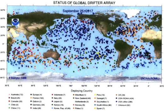
Alternatively, low-cost systems are operated in large numbers for collecting data in a distributed manner and broadcasted in near real-time via satellite communication. Under the coordination of international organizations and partnerships such as the World Meteorological Organization (WMO), approximately 1,400 drifter buoys ([21]

and figures 1-2f and 1-3a) are deployed over the oceans and monitor sea surface prop-erties, including temperature, current, wind, salinity, etc. Under the Argo program

(23)

10

20

30

40

50

Figure 1-1: Total number of months with f C02 values per 1*x 1 grid cell for 1970 through 2014 in SOCAT version 3, from [1].

([22] and figure 1-3b), about 4,000 profiling floats map the temperature and salinity of the ocean (figure 1-3). More recently, autonomous long-range, small (~ 3 m in

length) surface vehicles capable of following preset path (as opposed to the drifting buoys) have been developed. The Wave Glider [23], an autonomous surface vehi-cle that utilizes wave and solar energy for propulsion, is capable of multi-thousand mile long missions at a travel speed of -1.5 kts. The Saildrone (figure 1-2c), an autonomous sailboat can travel at up to 5 kts and has been successfully deployed in the Bering sea [24.

1.1.3 An energy-driven speed-size barrier

Despite these recent successful developments, ocean monitoring systems sufficiently cost-effective to be operated in swarms are too slow to capture fast phenomena such as fronts, or monitor rapidly developing unplanned events such as oil spills and toxic algal blooms. Furthermore, they may not cover enough ground to justify carrying

(24)

(a) Ocean data acquisition (b) Ocean data acquisition with

with satellites. Here: ESA's airplanes. Here: Meteo France's

Sentinel-1 satellite for the mea- Safire platform for meteorologic

surement of ocean waves. research.

(c) Ocean data acquisition

with autonomous wind-powered ships. Here: saildrone.

(d) Ocean data acquisition with

survey ships. Here: Research vessel from the UK's Natural Environment Research Council.

(e) Ocean data acquisition

un-derwater gliders. Here: a

glider operated by the Woods Hole Oceanographic Institution

(WHOI). Underwater gliders

are propelled by buoyancy con-trol.

(f) Ocean data acquisition

with survey langrangian sys-tems. Here: a drifter measures local properties and communi-cates them via satellite commu-nication.

(25)

high-performance sensors when spatial variability is important. An ideal complement to existing technologies would take the form of a low-cost, small 0(1-3) m, long dis-tance autonomous system. The main challenge resides in a energy-driven speed/size barrier: small-scale system lack the fuel carrying capability to satisfy the energetic requirements of fast, long-range travel. Conversely, high-speed, today's engineered long-range systems carry their own fuel and are high-cost, large systems 0(10-30) m. Alternately, if a small-scale system was able to continuously extract enough power from the oceanic environment (solar, wind or wave), it could break the speed-size barrier.

As will be discussed below and throughout this thesis, speed-size barrier is actually broken by a biological system, the albatross (figure 1-5). Up to over three meters in span and 10 kg in weight, albatrosses use wind for propulsion. After a general discussion on the general principles of wind power, the main aspects of the wandering albatross and its flight will be discussed.

1.1.4 Wind power energetics, a unified approach

Wind energy extraction relies on a transfer of momentum between media of different speeds. Consider for the sake of the discussion two fluid media initially moving uni-formly at velocities W1 and W2. Assume that a device is able to transfer momentum

between the two media. For simplicity, suppose that at each time instant the device interacts with an element of mass dmi of medium i = {1, 2} , and modifies its velocity

by a small amount wi. The momentum change of medium i during the time instant is dpi = dmiwi, and the force by the device onto medium i is F = g = ?itwi. The total rate of change in kinetic energy of the two media is

() 1

(26)

STATUS OF GLOBAL DRIFTER ARRAY

9'N September 5,"217

60'N

4, 0 0

W0E 60 E W0E i2WE IW0E 1W0 1W0W 120'W W0W 60*W W0W 0' 3WE

Deploying Country

* Aambuie(72) S Eurcp.(4) S IISOnISuiB(?) S MmaUrus(1) Peaull) * UK(39)

.*.- -lz(S Prmfic(0) .*.HSiy2) .NOW Zgilind)4g) *Sanugal? 0 USA-NOAA I424) * Ca..(ZS) 0 GubOW(Z *Jae (6 N.Iwdmnd.3 0 Seychewbs( 0 USA-OUW(Z2S

-cmi.(S 0 omwin(34) S Enya is) * Nmy(Ey ( 0 South Atiea(86) * Unkntown(O2)

* CI~i (1) 0 Ir...a) .Korms,Rep of(45) * Palu(1) *Spak,(7)

(a) Array of the global drifter program. The drifters measure the near-surface water properties and currents.

60N 3777 Fos

30'S

60E 120'E 180i 120 W 60'W 0.

(b) _{Array of floats in the Argo program. The floats perform periodic dives in}

order to profile the water column.

(27)

Kinetic dmiwW1 Energy Wind ₁ (W, _wW 1 W2 2 4. idmiW₁-drntwiv

aU

Windrc h ~ ud ce nk" b onI b me C

Ai

I'lld on eee GrOUM for Kinetic d ~dmw(Wi -W ₂) Energy Win {dmW2 _2dmWw ₂ dm~w ftw",y 14yer e A Wind in keMa of Lkeei V bUi g

Figure 1-4: Wind power energetics. Albatross credits: Raja Stephenson.

If the device transfers momentum between the two media (rather than accumulating

it), it follows that F1

+

F2 = 0 and that P simplifies into

P=F1 - (W 1-W 2)- (wi - w2)) (1.2)

In the limit of small loadings wi -+ 0 and rni = Wi - 00 (such that Fi remains

constant), power extracted further simplifies to

P = F1 - (W1- W2). (1.3) This relationship does not depend on the inertial frame of reference in which the velocities are calculated, and energy is extracted if the force causing the transfer of momentum tends to reduce the velocity inhomogeneity (Figure 1-4e).

It is often convenient to consider the energetic exchange in a frame of reference where W2 = 0 and W1 = W. In this frame, a force F1 oc -W extracts energy by

slowing down medium 1 and accelerating medium 2. Consider then Equation (1.1) with W2 = 0 in the the regime of small loadings w, = w

<

W, as illustrated in

(28)

Figure 1-4a. The energy loss of medium 1 is m1W -w + O(w2). It is first order in

w. Let K = (ml/M2)2_{. The energy gain of medium 2 is irs}

2w

2_/2. _{It is second order}

in w, and therefore much smaller than the energy loss of medium 1. In other words, the loss of kinetic energy of the fast medium is linear with the momentum tranferred while the gain of the slow medium is only quadratic, such that the system's energy decreases. Note also that Equation (1.3) takes the well-known and intuitive form

P=F-W (1.4)

with F = miw.

For instance a wind turbine (Figure 1-4b) operates by transferring momentum from the atmospheric wind to the ground. Analyzed in ground frame, the system is such that on the one end the turbine's rotor slows down the wind layer initially at a speed W by an amount w while on the other end, the tower's base applies a force onto the still ground, that tends to accelerate it (by an infinitesimal amount w2 ~ 0 since the ground has a very large mass). If the mass rate of the atmospheric wind is 7h, the

loss of kinetic energy of the system {Wind layer + Ground} is P = -maW(W - w/2)

and reflects energy extraction by the wind turbine.

Sailboats (Figure 1-4c) are wind-powered systems and their energetics obey the same principles, by transferring momentum from wind layer to the water. Indeed, neglecting drag forces, on the one hand the sail slows down the wind layer while on the other hand the underwater keel transmits that momentum to the water. When traveling crosswind, basic trigonometry (figure 1-4f-drag forces are omitted) shows that power extraction follows Equation (1.3) in the particular form P = Fthrust -U =

LkeelW, where U is the sailboat velocity and Lkeel the lift force generated by the keel,

approximately equal in intensity to that generated by the sail. In the large lift-to-drag ratio regime or when the lift-to-drag is dominated by the water lift-to-drag, the speed of the crosswind sailboat is

Keel lift (1.5)

Total drag

(note that for large lift-to-drag ratios, Lkeel e Lsaii). Even for small lift-to-drag

(29)

ratios this relation qualitatively reflects the important aspects of crosswind sailboat propulsion.

Recently, wind-powered machines that travel directly downwind faster than the wind (DDWFTTW) have been developed (Figure 1-4d). While it may sound counter-intuitive that a wind-powered system could be able to travel faster than the wind, as shown in Equation (1.3), as long as a transfer of momentum that tends to reduce inhomogeneity between two media of different velocities, energy is extracted [25]. A successful implementation of a DDWFTTW machine operating on land had a pro-peller acting to slow down the wind (thereby generating trust), that was directly linked to the vehicle's wheels [26]. The torque required to rotate the propeller origi-nated from the ground's traction on the wheels.

Overall, all the systems considered have three functional elements: a "gravity-canceling" element (buoyant or planning hull for sailboats, tower foundation for the wind turbine, etc.), a "sail-like" element that slows down the fast layer and a "keel-like" elements that transfers the momentum to the slow layer. For instance, for the wind turbine, the sail element is the blades and the keel element is the tower's foundations.

1.1.5 The albatross, a wind-powered drone

The wandering albatross (diomedea exulans, figure 1-5), the largest living bird on the planet, is the size of a small drones at a typical 8-10 kg and 3 m span [27]. Mostly found in the southern oceans between 30* and 600 S (figure 1-6), where strong winds prevail, albatrosses fly by extracting their propulsive energy from the wind through a specific flight technique called dynamic soaring. They typically travel 500 miles per day [28]. While for most migrating birds, flying is a very energy intensive endeavor (they may lose up to 50% of their body weight during a migration [29]), the metabolism of a flying albatross is only slightly above baseline [30], suggesting that very little self energy is spent for flight. Albatrosses have been recorded to perform

dynamic soaring in winds from ~ 5 - 10 m/s up to at least Beaufort 9 (i.e. - 25m/s

(30)

(77*

xs,

- P -F

Figure 1-5: Albatross in flight Top: Wandering. Bottom: Salvin's (unverified). Cred-its: Raja Stephenson.

(31)

M Amsterdam Albatross E Short-tailed Albatross

1Fg - Antipodean Albatross U Shy Albatross s. r : . Blach-browed Albatross Sooty Albatross

AtBlack-footed Albatross Northern Giant-petrel

-- Buller's Albatross b

Southern Giant-petrely

s Chatham Albatross U Northern Royal Albatrott

s Gibsongs Albatross Southern Royal Albatross A sd r Grey-headed Albatross r Tristan Albatross d V

.r Indian Yellow-nosed Albatross d

Wandering Albatross

a Laysan Albatross U White-chinned Petrel

A Light-mantled Albatross g

Figure 1-6: Global distribution of some albatrosses species. Source: [2]

1.1.6 _{Wind propulsion of the albatross: dynamic soaring}

Albatrosses fly in the first 20 meters of the atmosphere above the ocean surface. There, the wind is inhomogeneous in a somehow predictive way: on average the wind is slower close to the water surface-where the no-slip boundary condition at the surface necessitates that the air and water have the same velocity at the interface-and faster higher in altitude. In some conditions the average wind profile approximately follows the logarithmic law of the wall [3 1, 32]. The wind speed is also influenced by interactions with the wave field of the ocean. The wave-wind coupling is a complex topic and a subject of active research [3, ,4 ] but some properties emerge: if the

airflow separates at wave crests' a slow recirculation region develops behind the wave crest. In the linear regime, if the airflow remains attached to the water surface the

inhomogeneous wind field follows a known linear partial differential equation [35]. Accordingly, the low-altitude wind field is inhomogeneous. The albatross' dy-namic soaring consists of a characteristic s-shaped, up-down, flight pattern which redistributes the wind momentum between the fast region in altitude and the slow region near the surface.

This thesis is dedicated to understanding how the transfer of momentum takes places, and how the albatross' flight can inform the design of wind-powered flying robots, and more generally high-performance systems operating at the air-water in-terface.

(32)

1.2 Chapter overviews

The thesis is divided in two main parts. The first part (chapters 2 and 3) studies the flight dynamics of the albatross and more generally dynamic systems. The second part (chapters 4 to 6) discuss how the principles of dynamic soaring may be inform the design of wind-powered robots.

Part 1 starts with chapter 2, which closely parallels [36]. GPS recordings of flying albatrosses from the published literature are compared with dynamic soaring trajectories obtained by numerical trajectory optimization. It is found that contrary to the prevailing theory that explains dynamic soaring as a succession of half turns in the slow and fast layers of the wind field, but in accordance with trajectories of flying albatrosses, the optimal trajectory is a succession of shallow arcs where the glider remains nearly crosswind at all times. An analytic solution for the optimal, minimum-wind trajectory is computed in the thin shear limit. The analytic solution lends itself well to an intuitive analogy between the dynamic soaring maneuver and sailing. In dynamic soaring, the glider successively plays the role of a sail and that of a keel.

In chapter 3, the mathematical model of chapter 2 and the analytic solution in the limit of thin shear layers are expanded asymptotically to shear layers of finite thickness. An analytic asymptotic expansion describing the optimal, minimum-wind trajectory of dynamic soaring is exhibited and validated against numerical optimiza-tion trajectories from chapter 2 and the literature, as well as in-flight recordings or albatrosses. Chapter 3 closely parallels [37].

Opening part 2, chapter 4 is dedicated to the modeling and control of a flexi-ble, vertical, surface piercing hydrofoil actuated in pitch for the general use of such appendages in high-performance ocean surface robotic applications. A time-varying hydrodynamic model is derived for the hydrofoil dynamics, and a feedback lineariza-tion controller based on force, velocity and immersion depth measurement is proposed and tested on a prototype towed at 6-10 m/s. Chapter closely parallels [3S].

(33)

of wind-powered propulsion of albatrosses and sailboats. Three important charac-teristics emerge: the capability to utilize the full extent of the wind intensity, the system's lift-to-drag ratio and the property of "weak coupling" to the surface which potentially allows small-scale systems to operate in strong seas. It is suggested fitting an albatross-like glider with a vertical, surface-piercing hydrofoil keel would lead to a system performing well along all the aforementioned characteristics. The chapter ends with high-level descriptions of several possible embodiments of such a system-among which an "amphibious dynamic soaring glider" and a "flying sailboat"-and a discussion on possible modes of operation.

Chapter 6 presents a quantitative study of a flying sailboat system. It closely parallels [391. The trim flight performance is derived and evaluated for a 3.4 m span, 3 kg system. A flight controller for precise low-height longitudinal control is proposed. The longitudinal controller is combined with the hydrofoil controller of chapter 4. Finally, the critical maneuver of the flying sailboat, which is the capability to fly at extreme low height above the water surface, immerse the keel in the water and utilize it to generate a controlled side lift force, is demonstrated experimentally on a prototype.

(34)

Part I

(35)

Chapter 2 Optimal dynamic soaring consists of

successive shallow arcs

Abstract

Albatrosses can travel a thousand kilometers daily over the oceans, through a dynamic maneuver. They extract their propulsive energy from horizontal wind shears with a flight strategy called dynamic soaring. While thermal soaring, exploited by birds of prey and sailplanes, consists of simply remaining in updrafts, extracting energy from horizontal winds necessitates redistributing momentum across the wind shear layer,

by means of an intricate and dynamic flight maneuver. Dynamic soaring has been

described as a sequence of half-turns connecting upwind climbs and downwind dives through the surface shear layer. This chapter investigates the optimal (minimum-wind) flight trajectory, with a combined numerical and analytic methodology. It is shown that contrary to current thinking, but consistent with GPS recordings of albatrosses, when the shear layer is thin the optimal trajectory is composed of small-angle, large-radius arcs. Essentially, the albatross is a flying sailboat, sequentially acting as sail and keel, and most efficient when remaining crosswind at all times. The present analysis constitutes a general framework for dynamic soaring and more broadly energy extraction in complex winds.

2.1 Introduction

Dynamic soaring is the flight technique where a glider, either a bird a machine, ex-tracts its propulsive energy from non-uniform horizontal winds such as those found over the oceans. Wandering albatrosses (diomedea exulans), the archetypal dynamic

(36)

soarers, have been recorded to travel 5,000 km per week while relying on wind energy alone [2s, 40, 30]. The engineering potentialities of dynamic soaring are

tantaliz-ing: a robotic albatross could survey the oceans (or ride the wind shear of the jet stream [I I ]), and collect oceanic and atmospheric data, traveling at over 40 knots with a virtually infinite range [142,

13].

A major obstacle to intelligent robotic soaring has resided in the complexity of

the wind power extraction process that, by nature, requires planning on-the-go an energy positive trajectory in a stochastic, hard to measure, and poorly understood wind field. Conversely, progress in the description of dynamic soaring energetics can help design efficient algorithmic solutions to the online trajectory planning problem. Improving the understanding of dynamic soaring is also important in avian ecology. In particular, it allows to better evaluate the impact of climate change on the behavior and habitat of albatrosses, petrels, and other pelagic birds, that are dependent on specific wind conditions [4].

At the meso-scale, it was shown that the vast majority of the wandering albatross' flight is performed in an overall cross- or downwind direction, by dynamic soaring [30]. Although on relatively rare occasions (attributed to foraging [41), they may fly up-wind, in those instances they typically need to provide propulsive power. As far as dynamic soaring is concerned, crosswind flight (i.e. when the average airspeed is or-thogonal to the average wind direction) is the dominant mode, and the focus of this

chapter.

In the first attempt to describe dynamic soaring, Rayleigh [46] modelled the wind profile (figure 2-1) as a still boundary layer separated from the above windy free stream blowing at WO by an infinitely thin shear layer (see figure 2-1c, hereafter Rayleigh's wind model). He noticed that when traversing the shear layer up- or downwind, the albatross' groundspeed is conserved but its airspeed is not, and may increase by up to WO. Rayleigh connected up- and downwind transitions with 1800 half-turns in order to construct an energy neutral trajectory (hereafter Rayleigh's cycle, figure 2-2b and e.g. [.47]): at each transition, the airspeed gain compensates for the inherent losses due to drag. Because the drag is quadratic with airspeed,

(37)

a limit cycle is reached. This description of the dynamic soaring trajectory, based on phases of flight directly up- or downwind connected by half-turns, has carried

on until today [18, 19, 50, 51, 52, 53, 5 1, 17, 55, 56, 57, 58] in two energetically

equivalent forms: trajectories with constant turn direction are O-shaped, or loitering; trajectories with alternating turn directions are S-shaped, or traveling.

Recently published observations based on high-accuracy GPS measurements [2;, 4, 5] (reproduced in figures 2-2a and 2-4) show that albatrosses in crosswind flight do not follow half-turns, but rather an elongated, albeit oscillating, trajectory. As we report below, analysis of this data shows that they typically turn by only 50-70*, about a third of the Rayleigh's 1800 half-turn.

The aim of this chapter is to build a model of dynamic soaring that addresses the 3x factor discrepancy in turn amplitude between the half-turn explanation and published field data of flying albatrosses. To this end, we computed the "minimum-wind trajectory", i.e. the most efficient trajectory of dynamic soaring in the sense that it requires the least amount of wind to allow sustained flight, and investigated the variation of its shape with the thickness of the shear layer. We discovered that contrary to prevailing theory, the most efficient trajectory in the thin shear layer regime is a sequence of arcs of vanishingly small angle, with the direction of flight nearly crosswind at all times. We were able to explain this observation analytically, lowering the wind required for dynamic soaring by over 35% compared to previous models [A 2].

2.2 Methods

2.2.1 Wind model

In the last two decades, a popular approach has attempted to perform accurate nu-merical modelling of the albatross flight in logarithmic or power law profiles, deemed good models of the average wind field in the first 20 m above water, where the alba-tross flies. However, in this framework it has been shown [7, 59] that dynamic soaring

(38)

W(z) WO Rayleigh 1+e-z/6 _Model 10 Wind/Free-stream

<ayer

5

- --.... ... ... .

- hear layer _herlyrzf 0 _{< 36} _{No wind itf}

5- - separated para _region slow layer

1 b,

<< -6

-10 L._ I.

0 woo

WO

w w

Figure 2-1: Wind profile. (a) Wind field behind waves. Color-coding: wind inten-sity. Experimental data adapted from [3]. (b) The logistic wind profile in this study captures adequately the wind field in separated regions, such as belind ocean waves. More generally, it constitutes a robust way to approximate a wide class of wind fields, based on two parameters: a typical wind speed inhomogeneity Wo separated by a shear layer of typical length-scale 6. (c) Rayleigh's wind model is the limit of the logistic profile for 6 -+ 0.

is extremely sensitive to the wind field in the first meter above the surface, precisely where wind-wave interactions and temporal variability make the logarithmic model

less relevant.

In contrast, Rayleigh's discontinuous wind model embraces the sharp wind shear

that exists in separated regions, such as behind breaking waves or mountain ridges. Recent studies suggest that wind separation in ocean wave fields may be more frequent than previously believed ([i] and figure 2-1a), further reducing the relative merit of log-based descriptions.

In this study, rather than attempting to conduct high-fidelity, high-complexity modelling of dynamic soaring for a specific system, we aim for a general and robust analysis of the principles of dynamic soaring, whose main conclusions should hold independently of the details of the wind field or glider. This approach is in part motivated by the fact that despite the significant stochasticity of the wind field in which albatrosses fly, their trajectory is quite regular. With this in mind, the wind profile, which varies with altitude z, is modelled by means of a logistic function (figure 2-1b) parameterized by the free stream wind speed WO and the shear layer

(39)

a Wind 7.8m/sfN. _/ _{Albatross ground speed 16.3m/s} loom b c d Wind Wind Continuous U du e todgIn wind ay Instantaneous V

a*C in boundary yer

S du to drag

Topview Soundary layer TOp vew Boundary laer

Figure 2-2: The albatross' trajectory. (a) Recording of a flying albatross from [4] (top view). In crosswind flight the typical turn of the albatross is about 50-70o.

Dot-dashed yellow portions of the trajectory: the albatross is involved in a 600 turn within

+200. Dashed red portions: the albatross is involved in a 600 turn within t100. Note

that while in the ground frame the mean albatross travel has a downwind component, in the frame moving with the average wind it is nearly crosswind. (b) The Rayleigh cycle describes the albatross' flight as a sequence of half-turns between the windy and slow regions. At each layer transition, there is an airspeed gain equal to the wind speed, which compensates inherent drag losses that are quadratic in airspeed. However this trajectory is suboptimal for energy extraction. Instead, for thin shear layers, the optimal cycle (c) is composed of a succession of small-angle arcs. The flight portion in the wind layer is functionally analogous to the sail of a sailboat,

Dynamic soaring beyond biomimetics: control of an albatross-inspired wind-powered system