Distributed method selection and dispatching of contingent, temporally flexible plans

Distributed Method Selection and Dispatching of

Contingent, Temporally Flexible Plans

by

Stephen Block

Submitted to the Department of Aeronautics and Astronautics

in partial fulfillment of the requirements for the degree of

Master of Science in Aeronautics and Astronautics

at the

MASSACHUSETTS INSTITUTE OF TECHNOLOGY

February 2007

@

Massachusetts Institute of Technology 2007. All rights reserved.

A u th o r

.. ...

Department of Aeronautics and Astronautics

February 1st, 2007

Certified by...

Brian C. Williams

Associate Professor

Thesis Supervisor

Accepted by.

...

\

\

Jaime Peraire

Professor of Aeronautics and Astronautics, Chair, Committee on

Graduate Students

MASSACHUSETTS INSTTWUTE OF TECHNOLOGY

MAR 2 8 2007

AERO

Distributed Method Selection and Dispatching of

Contingent, Temporally Flexible Plans

by

Stephen Block

Submitted to the Department of Aeronautics and Astronautics on August 25, 2006, in partial fulfillment of the

requirements for the degree of

Master of Science in Aeronautics and Astronautics

Abstract

Many applications of autonomous agents require groups to work in tight coordination. To be dependable, these groups must plan, carry out and adapt their activities in a way that is robust to failure and to uncertainty. Previous work developed contingent, temporally flexible plans. These plans provide robustness to uncertain activity du-rations, through flexible timing constraints, and robustness to plan failure, through alternate approaches to achieving a task. Robust execution of contingent, temporally flexible plans consists of two phases. First, in the plan extraction phase, the executive chooses between the functionally redundant methods in the plan to select an execu-tion sequence that satisfies the temporal bounds in the plan. Second, in the plan execution phase, the executive dispatches the plan, using the temporal flexibility to schedule activities dynamically.

Previous contingent plan execution systems use a centralized architecture in which a single agent conducts planning for the entire group. This can result in a commu-nication bottleneck at the time when plan activities are passed to the other agents for execution, and state information is returned. Likewise, a computation bottleneck may also occur because a single agent conducts all processing.

This thesis introduces a robust, distributed executive for temporally flexible plans, called Distributed-Kirk, or D-Kirk. To execute a plan, D-Kirk first distributes the plan between the participating agents, by creating a hierarchical ad-hoc network and

by mapping the plan onto this hierarchy. Second, the plan is reformulated using a

distributed, parallel algorithm into a form amenable to fast dispatching. Finally, the plan is dispatched in a distributed fashion.

We then extend the D-Kirk distributed executive to handle contingent plans. Contingent plans are encoded as Temporal Plan Networks (TPNs), which use a non-deterministic choice operator to compose temporally flexible plan fragments into a nested hierarchy of contingencies. A temporally consistent plan is extracted from the

TPN using a distributed, parallel algorithm that exploits the structure of the TPN.

At all stages of D-Kirk, the communication load is spread over all agents, thus eliminating the communication bottleneck. In particular, D-Kirk reduces the peak

communication complexity of the plan execution phase by a factor of

0

(f),

0 (Nse) in the centralized case, to typical values

of 0 (N

_{e) per node and 0}

(

)

_{per agent in the distributed case, where N is the}

number of nodes in the plan and e is the number of edges per node in the input plan. Both of the above results were confirmed empirically using a C++ implementation of D-Kirk on a set of parameterized input plans. The D-Kirk implementation was also tested in a realistic application where it was used to control a pair of robotic manipulators involved in a cooperative assembly task.

Thesis Supervisor: Brian C. Williams Title: Associate Professor

Acknowledgments

I would like to thank the members of the Model-Based Embedded and Robotic

Sys-tems group at MIT for their help in brainstorming the details of the D-Kirk algorithm and for their valuable feedback throughout the process of writing this thesis. Partic-ular thanks are due to Seung Chung, Andreas Hoffman and Brian Williams. I would also like to thank my family and friends for their support throughout.

The plan extraction component of the work presented in this thesis was made possible by the sponsorship of the DARPA NEST program under contract

F33615-01-C-1896. The plan reformulation and dispatching components were made possible by the sponsorship of Boeing contract MIT-BA-GTA-1.

Contents

1.5.1 Distribution of the TPN across the Processor Network . . . . 28

1.5.2 Selecting a Temporally Consistent Plan from the TPN . . . . 29

1.5.3 Reformulating the Selected Plan for Dispatching . . . . 29

1.5.4 Dispatching the Selected Plan . . . . 34

1.6 Key Technical Contributions . . . . 36

1.7 Performance and Experimental Results . . . . 37

1.8 Thesis Layout . . . . 38

2 Robust Execution 39 2.1 Introduction . . . . 39

2.2 Temporally Flexible Plans . . . . 39

2.3 Dispatchable Execution . . . . 43

2.4 Temporal Plan Networks . . . . 57

2.5 Plan Extraction . . . . 58

2.6 Related Work . . . . 63 7

3 Plan Distribution 3.1 Introduction . . . . 3.2 Distribution . . . . 3.3 Communication Availability . . . . 4 Plan Reformulation 4.1 Introduction . . . . 4.2 Basic Structures and Algorithms . . . . 4.2.1 Simple Temporal Network . . .

4.2.2 Distance Graph . . . . 4.2.3 Distributed Bellman-Ford . . .

4.2.4 Predecessor Graph . . . . 4.2.5 Distributed Depth First Search 4.2.6 Post Order . . . . 4.3 Distributed Reformulation . . . . 4.3.1 Algorithm Structure . . . .

4.3.2 Processing of Rigid Components 4.3.3 Identification of Non-Dominated 4.3.4 Complexity . . . . 4.4 Conclusion . . . . 5 Plan Dispatching 5.1 Introduction . . . . 5.2 Distributed Dispatching . . . . 5.2.1 Algorithm Structure . . . . . 5.2.2 Waiting to Start . . . .

5.2.3 Waiting to Become Enabled

5.2.4 Waiting to Become Alive . . .

5.2.5 Executing . . . . 5.2.6 Complexity . . . . 5.3 Conclusion . . . . Edges 67 67 67 73 79 . . . . . 79 . . . . . 80 . . . . . 80 . . . . . 80 . . . . . 83 . . . . . 86 . . . . . 87 . . . . . 90 . . . . . 92 . . . . . 92 . . . . . 95 . . . . . 122 . . . . . 128 129 131 131 131 132 133 135 137 138 138 139

6 Plan Extraction 141

6.1 Introduction ... 141

6.2 Distributed Plan Extraction . . . . 141

6.2.1 Algorithm Structure . . . . 143

6.2.2 Candidate Plan Generation . . . . 146

6.2.3 Temporal Consistency Checking . . . . 158

6.2.4 Complexity . . . . 161 6.3 C onclusion . . . . 161 7 Results 163 7.1 Introduction . . . . 163 7.2 Performance Tests . . . . 163 7.2.1 Dispatching . . . . 164 7.2.2 Reformulation. . . . . 166

7.3 Real World Scenario . . . . 170

7.4 Conclusion. . . . . 171

7.5 Future Work. . . . . 172

List of Figures

1-1 _{This figure shows a cooperative assembly task where two manipulators,}

WAMO and WAM1, must deliver a tool to a drop-off location. The drop-off location is reachable by manipulator WAMI only. Pick-up locations 0 and 1 are reachable by manipulators WAMO and WAM1 respectively. Both manipulators can reach the hand-off location. . . 24

1-2 This figure shows a graph representation of a plan describing a coop-erative assembly task . . . . 27

1-3 This figure shows the trivial agent hierarchy for the two agents involved in the tool delivery task. The choice of WAMO as the leader is arbitrary. 28

1-4 This figure shows the TPN after distribution between the agents in-volved in the execution. White nodes are assigned to WAMO and gray nodes to W AM I. . . . . 30

1-5 This figure shows the STN corresponding to the temporally consistent plan selected from the TPN. . . . . 31

1-6 This figure shows the Minimal Dispatchable Graph for the coopera-tive assembly task plan. Many nodes have been eliminated as a result of collapsing Zero-Related groups, Rigid Components have been rear-ranged and the non-dominated edges have been calculated. Some edges to and from node 1 are shown as stepped lines for clarity. . . . . 33

1-7 This figure shows the Minimal Dispatchable Graph for the cooperative assembly task plan at time 5 during dispatching. Executed nodes are shown in dark gray, with their execution times. Other nodes are labeled with their current execution window. Enabled nodes which are not yet alive are shown in light gray. . . . . 35

2-1 This figure shows graph representations of the activity primitive and the RMPL parallel and sequence constructs used to build a tempo-rally flexible plan. (a) activity, (b) parallel and (c) sequence . . 41

2-2 This figure shows a simplified version of the plan from the manipulator tool delivery example used in Chapter 1 as an example of a temporally flexible plan. . . . . 42

2-3 This figure shows the distance graph representation of the simple tem-poral network from the example temtem-porally flexible plan introduced in Section 2.2. . . . . 45 2-4 This figure shows (a) a portion of the distance graph for the example

temporally flexible plan introduced in Section 2.2 and (b) its corre-sponding All Pairs Shortest Path graph. . . . . 46

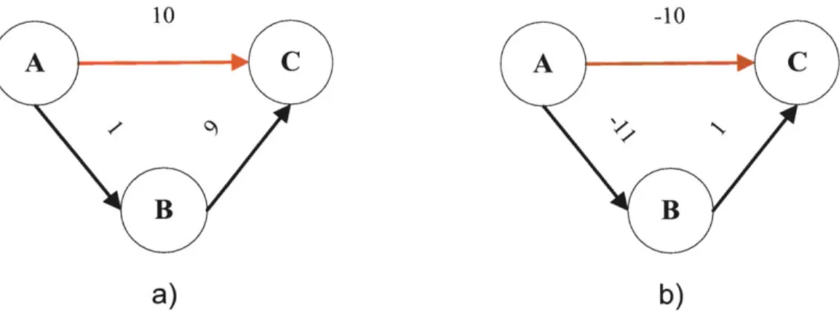
2-5 This figure shows an example of (a) an upper-dominated non-negative edge |ABI and (b) a lower-dominated negative edge

IABI

2-6 This figure shows the example plan with the RC consisting of nodes

27, 28, 29 and 30 highlighted in red . . . . 49

2-7 This figure shows the example plan with zero-related components col-lapsed in the RC consisting of nodes 27, 28, 29 and 30. . . . . 51 2-8 This figure shows the example plan with the RC consisting of nodes

27, 28, 29 and 30 processed. ... ... 53 2-9 This figure shows a snapshot of the dominance test traversal from node

1. The node being traversed is node 42. The dominance test applied

at this node determines that the APSP edge of length 10 from node 1 to node 42 is a member of the MDG. . . . . 55

2-10 This figure shows the RMPL representation of the manipulator tool delivery task. . . . . 59

2-11 This figure shows the graph representation of the RMPL choose con-struct used to build a Temporal Plan Network. The choice node is shown as an inscribed circle. . . . . 60

2-12 This figure shows the TPN representing the manipulator tool delivery scenario. . . . . 61 2-13 This figure shows an inconsistent plan. The distance graph contains a

negative cycle ABDCA . . . . . 62

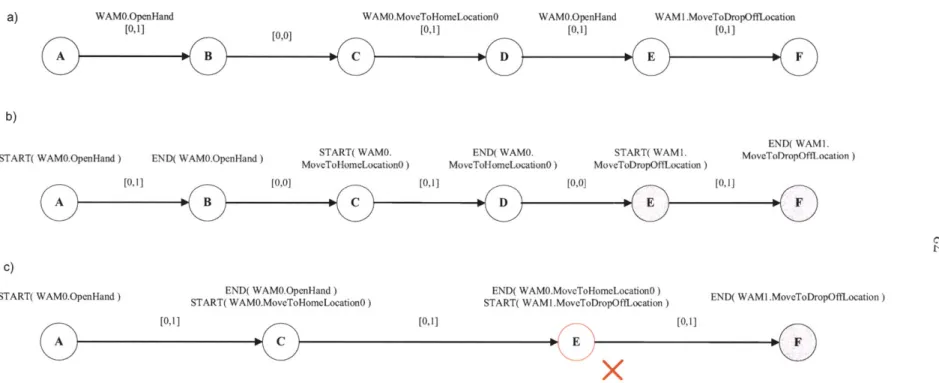
3-1 This figure shows an example plan fragment and how nodes are as-signed to agents based on the activities they will perform. (a) TPN with activities. (b) Activity start and end events assigned to nodes. (c) Nodes assigned to agents based on activity start and end events. Nodes assigned to WAMI are shown in gray. . . . . 69 3-2 This figure shows an example plan fragment that can not be distributed

because it requires events to be carried out simultaneously by multiple agents. (a) TPN with activities. (b) Activity start and end events assigned to nodes. (c) Nodes assigned to agents based on activity start and end events. Nodes assigned to WAMI are shown in gray. Node C can not be assigned because it owns activity events corresponding to activities to be carried out by both WAMO and WAMI. . . . . 70 3-3 This figure shows an example plan in which two ZR components must

be collapsed. (a) Before node assignment. (b) After node assignment. Nodes assigned to WAMI are shown in gray. (c) After collapsing. Node

E owns activity events corresponding to activities to be executed by

WAMO and WAMI so ZR component collapsing fails. . . . . 72

3-4 This figure shows the pseudo-code for the leader election algorithm used to form agent clubs. . . . . 74

3-5 This figure shows the operation of the club formation algorithm on a group of rovers. (a) Agents with communication ranges. (b) At time

1, agent 1 declares itself a leader and agent 2 becomes its follower. (c)

At time 3, agent 3 declares itself a leader and agents 2 and 4 become its followers. (d) At time 5, agent 5 declares itself a leader and agents 4 and 6 become its followers. . . . . 76 3-6 This figure shows the result of the tree hierarchy algorithm on a group

of rovers. The root of the tree structure is rover 3 and rovers 1 and 5 are its children. . . . . 77

4-1 This figure shows the Simple Temporal Network representation of the simplified plan from the manipulator tool delivery scenario and was first shown in Fig. 2-2. . . . . 81

4-2 This figure shows the distance graph representation of the Simple Tem-poral Network in Fig. 4-1 and was first shown in Fig. 2-3. . . . . 82

4-3 This figure shows the operation of the distributed Bellman-Ford algo-rithm on an example distance graph without any negative cycles. The start node is node A. (a) Input distance graph with initial distance estimates. (b) In round 1, nodes B and C update their distance es-timates. (c) In round 2, node D updates its distance estimate. (d) In round 3, node B updates its distance estimate and the values have converged. . . . . 84 4-4 This figure shows the pseudo-code for the distributed Bellman-Ford

algorithm . . . . 85

4-5 This figure shows the predecessor graph for the example distance graph in F ig. 4-3. . . . . 86

4-6 This figure shows the pseudo-code for the distributed Depth First Search algorithm . . . . 88

4-7 This figure shows the operation of the distributed Depth First Search Algorithm on the example distance graph from Fig. 4-3. Nodes are colored light gray once they have been visited and dark gray once their part in the search is complete. (a) The search begins at node A. (b) Node A sends a SEARCH message to its first outgoing neighbor, node B, which has no outgoing neighbors that have not been visited, so replies with a DONE message. (c) Node A then sends a SEARCH message to its other neighbor, node C. (d) Node C sends a SEARCH message to its only outgoing neighbor, node D. Node D has no outgoing neighbors that have not been visited, so replies with a DONE message. (e) Node C sends a DONE message back to node A. (f) The DFS is com plete. . . . . 89

4-8 This figure shows the operation of the distributed Depth First Search Algorithm, with the addition of RPO recording. The ID of the last posted node is included with each messages. Nodes are colored light gray once they have been visited and dark gray once their part in the search is complete and are labeled with the last posted node. .... 91

4-9 This figure shows the high-level pseudo-code for the distributed refor-mulation algorithm . . . . 93

4-10 This figure shows shows the distance graph representation of the plan describing the simplified manipulator tool delivery scenario and was first shown in Fig. 2-3. . . . . 94 4-11 This figure shows the pseudo-code for the rigid component processing

phase of the distributed reformulation algorithm. . . . . 95

4-12 This figure shows the distance graph with phantom node and corre-sponding zero length edges added. . . . . 97

4-13 This figure shows the SSSP distances from the phantom node and the corresponding predecessor graph. . . . . 98

4-14 This figure shows the predecessor graph for the first DFS, which starts at node 29 and records a post order of < 68, 1, 2, 3, 27, 28, 30, 29 >. 100

4-15 This figure shows the predecessor graph for the second DFS, which starts at node 31 and records a post order of < 33, 40, 32, 31 >. . . . 101

4-16 This figure shows the predecessor graph for the third DFS, which starts at node 34 and records a post order of < 35, 34 >. . . . . 102 4-17 This figure shows the predecessor graph for the fourth DFS, which

starts at node 36 and records a post order of < 37, 36 >. . . . . 103

4-18 This figure shows the predecessor graph for the fifth DFS, which starts at node 38 and records a post order of < 69, 67, 50, 41, 42, 43, 44, 45,

46, 47, 48, 49, 39, 38 >. . . . . 104 4-19 This figure shows the transposed predecessor graph for the example

plan, with the RC extracted by the first search, from node 38, highlighted. 107 4-20 This figure shows the transposed predecessor graph for the example

plan, with the RC extracted by the second search, from node 48, high-lighted. . . . . 108

4-21 This figure shows the transposed predecessor graph for the example plan, with the RC extracted by the eighth search, from node 31, high-lighted. . . . . 109

4-22 This figure shows the transposed predecessor graph for the example plan, with the RC extracted by the ninth search, from node 29, high-lighted . . . . 110

4-23 This figure shows the transposed predecessor graph for the example plan, with the RC extracted by the tenth search, from node 3, highlighted. 111 4-24 This figure shows the distance graph for the example plan, with RCs

circled, RC leaders highlighted and SSSP distances for each node. . . 114 4-25 This figure shows the distance graph for the example plan, with

zero-related component non-leaders shown dashed. . . . . 117

4-26 This figure shows the distance graph for the example plan, with the doubly linked chains of edges complete. . . . . 118

4-27 This figure shows the distance graph for the example plan after relo-cation of edges for the rigid component consisting of nodes 27 through

30. ... ... 120

4-28 This figure shows the distance graph for the example plan with RC processing complete. . . . . 121 4-29 This figure shows the pseudo-code for the dominance test traversal

phase of the distributed reformulation algorithm. . . . . 123

4-30 This figure shows the SSSP distances and predecessor graph from node

1 for the example plan. . . . . 125

4-31 This figure shows the predecessor graph from node 1 for the example plan, with the ID of the last posted node for DFS from node 1 recorded for each node. . . . . 126

4-32 This figure shows the predecessor graph from node 1 for the example plan, at the point where the traversal from node 1 has just passed node

69. MDG edges are shown in red. . . . . 127

4-33 This figure shows the complete MDG for the example plan. Edges from node 1 are shown as stepped lines for clarity. . . . . 128

5-1 This figure shows a state transition diagram for the distributed dis-patching algorithm . . . . 134

5-2 This figure shows the pseudo-code for the distributed dispatching al-gorithm . . . 135

5-3 This figure shows the MDG for the example plan at time 5 during dispatching. Executed nodes are shaded dark gray and enabled nodes are shaded light gray. Each node is labeled with its execution window in the case of a node which has yet to be executed, or its execution time in the case of an executed node. Some edges from node 1 are shown as stepped lines for clarity. . . . . 136 6-1 This figure shows the TPN for the tool delivery scenario introduced in

Chapter 1 and was first shown in Fig. 1-2. . . . . 142

6-2 The activity-sequence, parallel-sequence and choose-sequence con-structs used by the distributed plan extraction algorithm. . . . . 145

6-3 This figure shows the pseudo-code for the response of the start node v of a parallel-sequence network to a FINDFIRST message. . . . . . 148 6-4 This figure shows the search-permutations (node v) function. .... 149

6-5 This figure shows the pseudo-code for the response of the start node v of a parallel-sequence network to a FINDNEXT message. . . . . 150 6-6 This figure shows the pseudo-code for the response of the start node v

of a choose-sequence network to a FINDFIRST message. . . . . 151 6-7 This figure shows the pseudo-code for the response of the start node v

of a choose-sequence network to a FINDNEXT message. . . . . 152 6-8 This figure shows the TPN for the manipulator tool delivery scenario

during plan extraction when the temporal inconsistency is discovered at node 1. The deselected portion of the plan is shown in light gray. FINDFIRST messages are shown as blue arrows and ACK messages as green arrow s. . . . . 155 6-9 This figure shows the TPN for the manipulator tool delivery scenario

during plan extraction after node 2 has attempted to find a new consis-tent assignment in its currently selected subnetwork (nodes 51 through

66). The deselected portion of the plan is shown in light gray. FIND-NEXT messages are shown as black arrows and FAIL messages as red

arrow s. . . . . 157 6-10 This figure shows the TPN for the manipulator tool delivery scenario

at the end of plan extraction. The deselected portion of the plan is shown in light gray. FINDFIRST messages are shown as blue arrows,

FINDNEXT messages as black arrows, ACK messages as green arrows

6-11 This figure shows how the synchronous distributed Bellman-Ford

al-gorithm detects a temporal inconsistency as a negative cycle in the distance graph after N rounds. (a) Initial state for synchronous dis-tributed Bellman-Ford single source shortest path calculation from node A. (b) Single source shortest path distance estimates after round

1. (c) Single source shortest path distance estimates after round 2. (d)

Single source shortest path distance estimates after round 3. (e) Single source shortest path distance estimates after round 4 show failure to converge as a result of the negative cycle. (f) Single source shortest path distance estimates continue to vary after round 5. . . . . 162 7-1 This figure shows the results of the tests used to verify the performance

of D-Kirk with regard to communication complexity. The plot shows the peak number of messages sent by a node during dispatching as a function of the number of nodes in the plan. . . . . 165 7-2 This figure shows the results of the tests used to verify the performance

of D-Kirk with regard to computational complexity. The plot shows the average run time required by a node during reformulation. . . . . 168 7-3 This figure shows the results of the tests used to verify the performance

of D-Kirk with regard to computational complexity. The plot compares the average run time required by a node during reformulation for the centralized and distributed algorithms. . . . . 169

Chapter 1

Introduction

1.1

Motivation

The ability to coordinate groups of autonomous agents is key to many real-world tasks. An example scenario is the construction of a lunar habitat, where multiple robotic manipulators are required to work together to assemble the structure. For example, groups of manipulators may be required to act in coordination to lift large or heavy objects. A second scenario is an exploration mission on a foreign planet. This may involve multiple robots, each with a different skill set. For example, one robot with a high top speed may be sent ahead as a scout while a second, slower robot with a larger payload capacity is sent to the areas of interest discovered by the scout to collect samples. A final scenario is in manufacturing, where multiple robots simultaneously carry out different operations on a part. For example, one robot may hold a part in position while a second welds it to the main structure.

Coordinating such a group of agents involves executing an activity plan that de-scribes the actions each agent will perform. In order for the execution to be reliable we must provide robustness to unknown events and to disturbances. We provide robustness through an executive which performs dynamic execution of temporally flexible plans.

1.2

Previous Work

Previous work on robust plan execution has provided robustness to three types of unknowns: temporal uncertainty, execution uncertainty and plan failure.

Temporal Uncertainty. For many systems, the precise duration of an activity is

not fixed. It may be acceptable to conduct the activity for any period of time within a given range, or it may be the case that the duration of the activity is beyond the control of the executive. Temporally flexible plans [4] [19] allow us to accommodate both cases by modeling activities of uncertain duration. Use of these plans allows us to provide robustness to variation in the execution times of activities, as discussed below.

Execution Uncertainty. Traditional execution scheme assign execution times at

planning time, such that any temporal flexibility in the plan has been eliminated by dispatch time. This means that the executive is unable to adapt to uncertainty in execution times. To overcome this problem, while executing the plan in a timely manner, a dispatcher is used that dynamically schedules events. In particular, we use the methods of Tsamardinos et. al. [27], which are based on a least commit-ment strategy. This scheme is known as dispatchable execution [20], and provides robustness to execution uncertainty. Here, scheduling is postponed until execution time, allowing temporal resources to be assigned as they are needed. This allows the dispatcher to respond to the variable duration of activities at execution time. To minimize the computation that must be performed on-line at dispatch time, the plan is first reformulated off-line.

Plan Failure. Plan failure occurs when the temporal constraints in the plan are

such that no satisfying execution schedule can be found. To address plan failure, Kim introduced a system called Kirk [12], that performs dynamic execution of temporally flexible plans with contingencies. These contingent plans are encoded as alternative choices between functionally equivalent sub-plans. In Kirk, the contingent plans are represented by a Temporal Plan Network (TPN) [12], which extends temporally flexible plans with a nested choice operator. Kirk first extracts a plan from the TPN

that is temporally feasible, before executing the plan, as described above. Use of contingent plans adds robustness to plan failure.

Kirk uses a centralized architecture in which a single master agent is responsible for generating and executing an activity plan. In the case of a multi-agent plan, all other agents are inactive during the plan extraction phase. During plan execution, the other agents are simply instructed by the master agent to execute their activities at the relevant time. This means that the master agent must communicate with each agent at the time of execution of its activity and this creates a communication bottleneck at the master agent. As a result, the executive lacks robustness to communication latency. Similarly, the master agent may also suffer from a computational bottleneck, as it must process the plan for all of the agents involved in the plan.

Recent work by Wehowsky produced a distributed version of the plan extraction component of Kirk [31]. Prior to plan extraction, the TPN is distributed between the available agents. However, this work does not provide a distributed version of the reformulation or dispatching algorithms.

1.3

Problem Statement

The control of autonomous agents to achieve useful, real-world tasks requires activity plans that involve groups of agents. Reliable execution of these plans in an uncertain environment requires robustness to temporal uncertainty, execution uncertainty, plan failure and communication latency.

The problem solved by this thesis is to create a plan execution system for au-tonomous agents that is robust to these four types of uncertainty. The executive takes as input a multi-agent activity plan in the form of a TPN, extracts a temporally consistent plan from the contingencies available and schedules activities dynamically to respond to variable execution times. It does this in a way that avoids bottlenecks when communicating between agents.

1.4

Example Scenario

To motivate the discussion of our work, we introduce an example task taken from the lunar construction scenario. Consider the task of assembling a lunar structure using numerous robotic manipulators.

An example task which requires tight coordination of the manipulators is the delivery of a tool to a specific location, perhaps for use by a human astronaut. In this example there are two robotic manipulators. The action to be taken by the manipulators depends upon the initial location of the tool. For some initial locations, a single manipulator can pick up the tool and deliver it to the desired location. For other initial locations, both manipulators must work together: one manipulator picks up the tool and passes it to the second manipulator for delivery. This task is depicted in graphical form in Fig. 1-1. This example is used to demonstrate our work on a pair of Barret Technology's Whole Arm Manipulators (WAMs) in Section 7.3. For this reason, we refer to the two manipulators as WAMO and WAM1.

Tool

IL>"'

LJ

Pick-up location 0 Pick-up location 1

WAM 0 Hand-off location WAM 1 Drop-off location

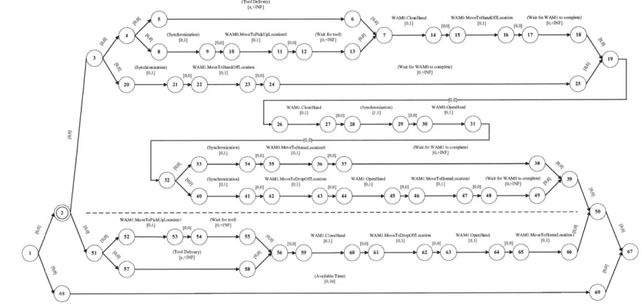
Figure 1-1: This figure shows a cooperative assembly task where two manipulators, WAMO and WAMI, must deliver a tool to a drop-off location. The drop-off location is reachable by manipulator WAMI only. Pick-up locations 0 and 1 are reachable

by manipulators WAMO and WAM1 respectively. Both manipulators can reach the

1.5

Proposed Approach

We address this problem with a distributed architecture in which all agents partici-pate in the execution process. Agents communicate by sending and receiving messages and this communication is spread evenly between all agents. This evens out commu-nication requirements and eliminates the commucommu-nication bottleneck, thus providing robustness to communication latency. We distribute computation between all agents to reduce computational complexity and to take advantage of parallel processing, thus improving performance relative to the centralized architecture. The greater the number of agents that is involved in the plan, the greater the extent to which the execution process can be shared out, so the greater the performance improvements.

Finally, our distributed architecture provides a framework for a future distributed system capable of providing robustness to loss of an agent during plan execution. Such a system would detect failure of an agent participating in plan execution, redistribute the plan over the remaining agents, re-plan if necessary, and continue execution.

Our proposed executive is a distributed version of Kirk, called D-Kirk, which performs distributed execution of contingent temporally flexible plans. D-Kirk consists of the following four phases.

1. Form a structured network of agents and distribute the TPN across the network

2. Select a temporally consistent plan from the TPN

3. Reformulate the selected plan for efficient dispatching

4. Dispatch the selected plan, while scheduling dynamically

The four phases are described below in the context of the manipulator tool de-livery task introduced above. A comprehensive summary of the reformulation and dispatching phases of execution in the centralized case is provided by Stedl [25].

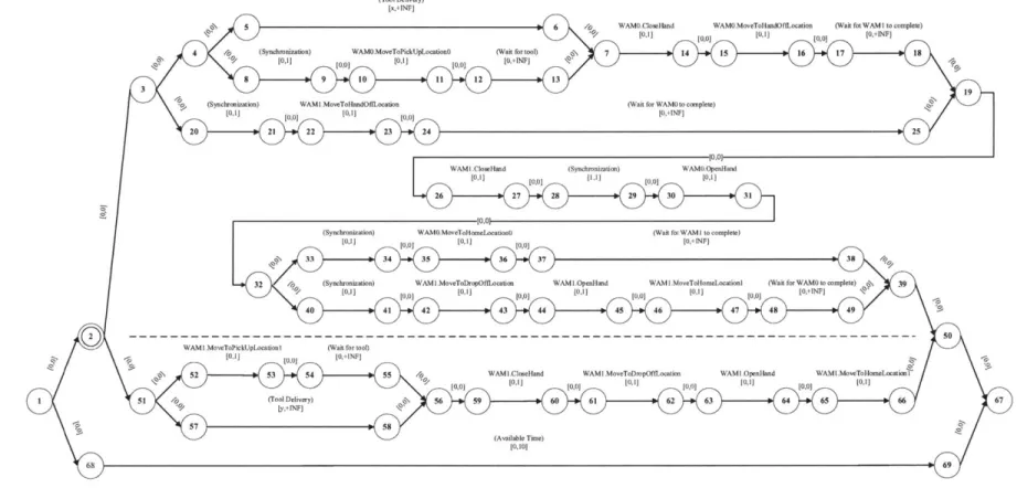
A TPN representing the tool passing task for a pair of WAMs is shown in graphical

form in Fig. 1-2. Nodes represent time events and directed edges represent simple temporal constraints. A simple temporal constraint [1, u] places a bound t+ -t E [1, u]

on the temporal duration between the start time t- and end time t+ of the activity or sub-plan to which it is applied.

The objective of the plan is to deliver the tool to the drop-off location, which is reachable by WAMI only. A tool is available at pick-up locations 0 and 1, but the time at which the tool becomes available at each location is unknown until execution time. Depending upon the time at which the tool becomes available at a particular location, it may not be possible to deliver the tool from that pick-up location to the drop-off location within the time bounds specified by the plan. Therefore, the plan contains two contingencies; one in which the tool from pick-up location 0 is used, and another in which the tool from pick-up location 1 is used. At execution time, the executive selects a contingency, if possible, which guarantees successful execution of the plan. The contingencies are represented in the plan by the single choice node, node 2.

In the case where the tool is at pick-up location 0, which is reachable by WAMO only, the task can only be completed if the manipulators cooperate. This contingency is shown in the upper half of Fig. 1-2. First, WAMO moves its hand to pick-up location

0, where it waits for the tool to arrive. When the tool arrives, WAMO closes its hand

around the tool and moves the tool to the hand-off location. At the same time, WAM1 moves to the hand-off location. Having completed these activities, either WAM will wait until the other WAM has completed its activities. Next, WAMI closes its hand around the tool and one second after completing the close, WAMO begins to open its hand. Within a second of WAMO opening its hand, WAM1 moves the tool to the drop-off location, where it immediately opens its hand to release the tool and finally moves to home position 1. Simultaneously, WAMO moves directly to home position

0. Again, having completed these activities, either WAM will wait until the other

WAM has completed its activities, before the plan terminates.

In the case where the tool is at pick-up location 1, which is reachable by WAMI only, the task can be completed by WAM1 alone. This contingency is shown in the lower half of Fig. 1-2. First, WAM1 moves its hand to pick-up location 1, where it waits for the tool to arrive. Once the tool has arrived, WAM1 closes its hand around

[x,+INF]

-KT

the tool and moves it to the drop-off location, where it opens its hand to release the tool and finally moves to home position 1.

The simple temporal constraints [x,

+INF]

+INF],

6 and nodes 57 and 58 respectively, represent the time we must wait from the start

of the plan until the tool becomes available at pick-up locations 0 and 1 respectively. The values of x and y, the minimum wait times, are not known until execution time. The simple temporal constraint [0, 10] between nodes 68 and 69 imposes an upper bound of 10s on the overall duration of the plan.

1.5.1

Distribution of the TPN across the Processor Network

Our objective in distributing the TPN is to share the plan data between the agents taking part in the execution. We assume that tasks have already been assigned to agents and distribute the TPN such that each agent is responsible for the plan nodes corresponding to the activities it must execute.

Before we can perform the distribution, we must arrange the agents into an ordered structure. This structuring defines which agents are able to communicate directly and establishes a system of communication routing, such that all agents can communicate. In D-Kirk, we form a hierarchy of agents using the methods of Coore et. al. [2]. In the case of the tool passing example only two agents are involved in the plan, so the hierarchy is trivial and the choice of WAMO as the leader of the hierarchy is arbitrary. The agent hierarchy is shown in Fig. 1-3.

WAMO

WAMI

Figure 1-3: This figure shows the trivial agent hierarchy for the two agents involved in the tool delivery task. The choice of WAMO as the leader is arbitrary.

Having formed the agent hierarchy, we assign plan nodes to agents. White nodes are assigned to WAMO while gray nodes are assigned to WAMI, as shown in Fig. 1-4.

1.5.2

Selecting a Temporally Consistent Plan from the TPN

The simple temporal constraints [x,

+INF]

+INF]

For the purposes of this example, we assume that x = 1 and y = 20. This means that the lower bound on the execution time of the upper contingency is 2, which is less than the plan's overall upper time bound of 10. The lower bound on the execution time of the lower contingency, however, is 20, which exceeds the overall upper time bound. Therefore, D-Kirk selects the upper contingency, which involves the two manipulators working together. The resulting temporally consistent plan is shown in Fig. 1-5.

1.5.3

Reformulating the Selected Plan for Dispatching

Dispatchable execution retains the temporal flexibility present in the input plan throughout the planning process, allowing it to be used to respond to unknown ex-ecution times at dispatch time. However, this approach increases the complexity of dispatching, relative to a scheme in which execution times are fixed before dispatch-ing. To minimize the amount of computation that must be performed in real time during dispatching, we first reformulate the plan. The output of the reformulation phase is a Minimal Dispatchable Graph (MDG), which requires only local propagation of execution time data at dispatch time.

The plan extracted from the TPN can be represented as a Simple Temporal Net-work (STN) and every STN has an equivalent distance graph. In a distance graph,

[ ,+[Nfl

Figure 1-4: This figure shows the TPN after distribution between the agents involved in the execution. White nodes are assigned to WAMO and gray nodes to WAMi.

(TolDelivery)

[x,+NF]

/o WAMO.ClosHand WAMO.MoeToHandOffLocaion (Wait fot WAM I to complet)

'0/ [0,1] rnno [0,I] m m [0,+iNF]

(Wait for WAMO to omplete)

[0,-+INF]

(Wafifot WAM I to complee) [O,+INF]

(Available Time)

[0,10]

Figure 1-5: This figure shows the STN corresponding to the temporally consistent plan selected from the TPN.

nodes represent time events and directed edges represent a single temporal constraint. Specifically, each edge AB in the distance graph has a length or weight b(A, B) which specifies the constraint t

B - [A ; b(A, B), where t

A and tB are the execution times of nodes A and B respectively. Reformulation operates on the distance graph rep-resentation of the selected temporally flexible plan and the MDG is itself a distance graph. The MDG for the cooperative assembly task example is shown in Fig. 1-6.

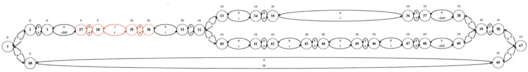
An important feature of the MDG is that all Rigid Components (RCs), that is groups of nodes whose execution times are fixed relative to each other, have been rearranged. In particular, the member nodes of the RC are arranged in a chain, in order of execution time, linked by pairs of temporal constraints. The member node with the earliest execution time, at the head of the chain, is termed the RC leader. All temporal constraints between the RC's member nodes and the rest of the plan graph are re-routed to the leader. Also, RC member nodes linked by temporal constraints of zero duration, are collapsed to a single node. Members of these Zero-Related (ZR) components must execute simultaneously, so any start or end events are transferred to the remaining node. An example of a rearranged RC is nodes 27 through 30 in Fig. 1-5. Nodes 27 and 28 and nodes 29 and 30 are ZR components, so are collapsed to nodes 28 and 30 respectively in Fig. 1-6. Node 28 is the RC leader so the edges between node 30 and nodes outside the RC are rerouted to node 28.

In the case of the fast reformulation algorithm used in D-Kirk, rearrangement of rigid components in this way is required for the correct operation of the algorithm used to determine the distance graph edges that belong in the MDG, as described below. Also, the rearrangement improves the efficiency of reformulation.

Once RCs have been processed, the reformulation algorithm identifies all edges that belong in the MDG. Some of the original edges of the input STN remain in the

MDG, while others are eliminated. In addition, the MDG contains new edges which

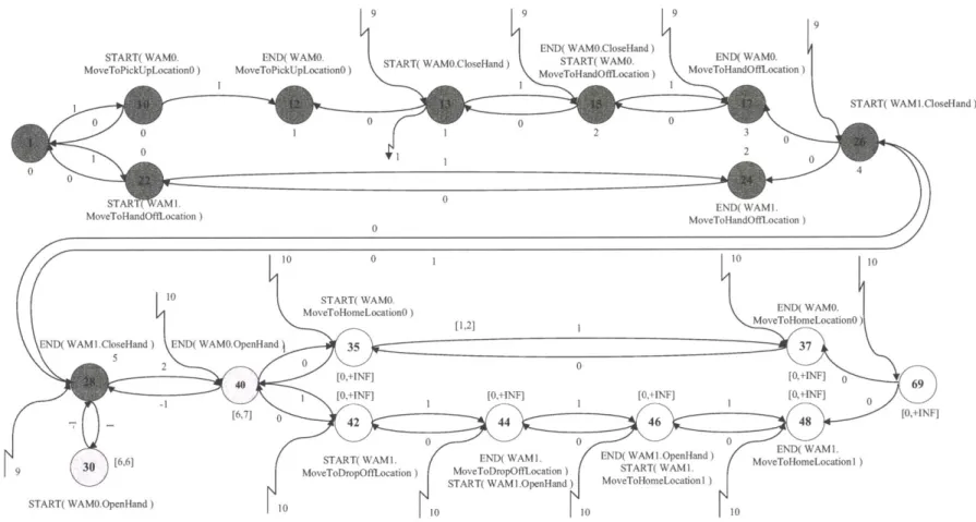
are required to make explicit any implicit timing constraints required for dispatching. An example of such an edge is that of length 9 from node 1 to node 13 in Fig. 1-6. It ensures that node 13 is executed sufficiently early that the upper bound of 10 units on the overall plan length can be met, given that later in the plan (between nodes 28

START( WAMI.CloseHand)

Figure 1-6: This figure shows the Minimal Dispatchable Graph for the cooperative assembly task plan. Many nodes have been eliminated as a result of collapsing Zero-Related groups, Rigid Components have been rearranged and the non-dominated edges have been calculated. Some edges to and from node 1 are shown as stepped lines for clarity.

and 40 in the MDG in Fig. 1-6) there exists a minimum duration of 1 unit.

During reformulation, the temporal constraints between the start and end nodes of an activity in the input plan may be removed if the constraints do not belong in the MDG, as described above. This means that activities no longer necessarily coincide with temporal constraints. For this reason, activities are instead represented as a pair of events: a start event at the start node and an end event at the end node. An example of this is the WAMO.OpenHand activity between nodes 30 and 31 in the

STN in Fig. 1-5, or equivalently nodes 30 and 40 in the MDG in Fig. 1-6.

1.5.4

Dispatching the Selected Plan

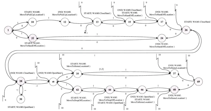
During dispatching each node maintains its execution window. The execution window is the range of possible execution times for the node, given the temporal constraints in the plan and the execution times of nodes that have already been executed. The start node, node 1 in the tool delivery example, is assigned an execution time of 0 by definition.

The dispatching algorithm uses an internal clock, the execution windows of the nodes and the temporal constraints from the MDG to determine when each node can be executed. We use a minimum execution time policy: where there exists a range of possible execution times, nodes are executed as soon as possible. When a node is executed the MDG edges are used to update the status of neighbor nodes.

A node must be both alive and enabled before it can be executed. A node is

enabled when all nodes that must execute before it have executed. A node is alive when the current time lies within its execution window. In addition, contingent nodes, which represent the end event of uncontrollable activities, must also wait for the uncontrollable activities to complete.

Fig. 1-7 shows a snapshot of the MDG for the tool delivery example during dis-patching at time 5. Executed nodes are shown in dark gray, with their execution times. Enabled nodes which are not yet alive are shown in light gray.

The distributed dispatching algorithm monitors the node for the enablement con-dition. The algorithm uses incoming EXECUTED messages from neighbor nodes

START( WAMI.CloseHand)

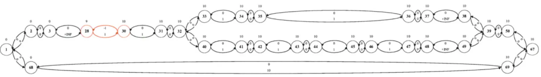
Figure 1-7: This figure shows the Minimal Dispatchable Graph for the cooperative assembly task plan at time 5 during dispatching. Executed nodes are shown in dark gray, with their execution times. Other nodes are labeled with their current execution window. Enabled nodes which are not yet alive are shown in light gray.

to update the enablement condition and the execution window. Once enabled, the algorithm waits for the current time to enter the execution window, while continuing to use EXECUTED messages to update the upper bound of the execution window. Once alive, and in the case of a contingent node, all uncontrollable activities ending at the node have completed, the node can be executed. Executing a node involves stopping all controllable activities that end at the node and starting all activities which start at the node. When a node is executed, EXECUTED messages are sent to its neighbor nodes so that they can update their execution window and enablement status.

For example, in Fig. 1-7, the last node to have been executed is node 28 at time

5. The non-positive MDG edges to node 28 from nodes 30 and 40 have been used

to enable these nodes and to update the lower bound of their execution window to 6 in each case. The positive MDG edges from node 28 to nodes 30 and 40 have been used to update the upper bound of the execution window of these nodes to 6 and 7 respectively.

1.6

Key Technical Contributions

D-Kirk performs distributed execution of contingent temporally flexible plans. The

technical insights employed by each phase of the algorithm are summarized below.

1. Distribute the TPN across the processor network. We arrange agents into a hierarchy to provide the required communication availability. We then map the TPN to the hierarchy, exploiting the hierarchical nature of the TPN

to maximize efficiency.

2. Select a temporally consistent plan from the TPN. We use a distributed consistency checking algorithm and interleave candidate generation and

consis-tency checking to exploit parallel processing.

3. Reformulate the selected plan for efficient dispatching. We use a

possible. The algorithm uses a state machine approach with message passing that is robust to variable message delivery times.

4. Dispatch the selected plan, while scheduling dynamically. The

algo-rithm uses a state machine approach with message passing that is robust to

variable message delivery times.

1.7

Performance and Experimental Results

The main objective of distributed D-Kirk is to eliminate the communication bot-tleneck present at the master node of the centralized architecture when the plan is dispatched. The peak communication complexity of the D-Kirk dispatching algo-rithm is 0 (e') per node or 0 (

'-)

that D-Kirk reduces the peak message complexity at dispatch time, when real-time operation is critical, by a typical factor of 0

(

D-Kirk also improves the computational complexity of the reformulation algo-rithm relative to the centralized case. The computational complexity is reduced from

o

)

Both of the above analytical results are verified by experimentation using a C++ implementation of D-Kirk operating on parameterized sets of plans of numerous types.

In addition, we use the C++ implementation to demonstrate the applicability of D-Kirk in a realistic setting. We use D-D-Kirk to execute the manipulator tool delivery example plan in our robotic manipulator testbed. This consists of a pair of Barrett Technology's Whole Arm Manipulators (WAMs), each with four degrees of freedom

and a three-fingered hand effector.

1.8

Thesis Layout

First, in Chapter 2, we review methods for the robust execution of contingent tempo-rally flexible plans. We discuss how dispatchable execution is used to robustly execute a temporally flexible plan, present a definition of a TPN and give an overview of plan selection in the centralized case. In Chapter 3 we present the first stage of D-Kirk; for-mation of an agent hierarchy to provide the required communication between agents and the distribution of the TPN over the group of agents. Chapters 4 and 5 present the details of the two stage process required by the dispatchable execution approach to execute a temporally flexible plan. First, reformulation, where the plan is recom-piled so as to reduce the real-time processing required at execution time. Second, dispatching, where the activities in the plan are executed. This is the core of the D-Kirk distributed executive. In Chapter 6 we extend the distributed executive to handle contingent plans. This completes the description of D-Kirk. Finally, in Chap-ter 7, we present experimental results which demonstrate the performance of Kirk and make comparisons with the centralized Kirk executive. We also demonstrate the real-world applicability of our solution by using D-Kirk to execute the manipulator tool delivery example plan in our manipulator testbed. Finally, we present conclusions and discuss directions for future work.

Chapter 2

Robust Execution

2.1

Introduction

This chapter serves as a review of methods used for robust execution of contingent temporally flexible plans in the centralized case. We first define a temporally flexible plan and its representation as a Simple Temporal Network (STN). We then review dispatchable execution, which provides a means to robustly execute a temporally flexible plan. We then present a definition of a Temporal Plan Network (TPN), which adds choices to a temporally flexible plan. This allows us to describe contingent plans, where each contingency is a choice between functionally equivalent threads of execution. We then review methods for selecting a temporally consistent plan from the TPN. Finally, we present related work on robust plan execution and distributed execution systems.

2.2

Temporally Flexible Plans

Traditional plans specify a single duration for each activity in the plan. A temporally flexible plan allows us to specify a range of durations, in terms of a lower and upper bound on the permissible duration. This allows us to model activities whose durations may be varied by the executive, or whose durations are unknown and are controlled

by the environment.

A temporally flexible plan is built from a set of primitive activities and is defined

recursively using parallel and sequence operators, taken from the Reactive Model-based Programming Language (RMPL) [32]. A temporally flexible plan encodes all executions of a concurrent, timed program, comprised of these operators.

A primitive element of a temporally flexible plan is of the form activity[l, u]. This

specifies an executable command whose duration is bounded by a simple temporal constraint. A simple temporal constraint [1, u] places a bound t+ - t- E [1, u] on the duration between the start time t- and end time t+ of the activity, or more generally, any sub-plan to which it is applied.

Primitive activities are composed as follows.

" parallei(subnetworki, .. . , subnetworkN) [1, u] introduces multiple subnetworks

to be executed concurrently.

" sequence(subnetwork, .. . , subnetworkN) [1, u] introduces multiple subnetworks

which are to be executed sequentially.

Note that the RMPL language also allows us to apply a simple temporal constraint between the start and end of a parallel or sequence operator, but this is purely syntactic sugar. In the case of the parallel operator, it corresponds to an additional parallel branch, consisting of a single activity with the prescribed simple temporal constraint. In the case of the sequence operator, it corresponds to an additional parallel operator, of which one branch is the sequence and the other is a single activity with the prescribed simple temporal constraint. For simplicity, we do not use these syntactic mechanisms in this thesis.

The network of simple temporal constraints in a temporally flexible plan form a Simple Temporal Network (STN). An STN is visualized as a directed graph, where the nodes of the graph represent events and directed edges represent simple temporal constraints. Graph representations of the activity primitive and of the parallel and sequence constructs are shown in Fig. 2-1.

Fig. 2-2 shows a simplified version of the selected plan from the manipulator tool delivery scenario used in Chapter 1 as an example of a temporally flexible plan. The

[1,u]

S

E

S

E

activity

parallel

A

z

Figure 2-1: This figure shows graph representations of the activity primitive and the RMPL parallel and sequence constructs used to build a temporally flexible plan.

(a) activity, (b) parallel and (c) sequence

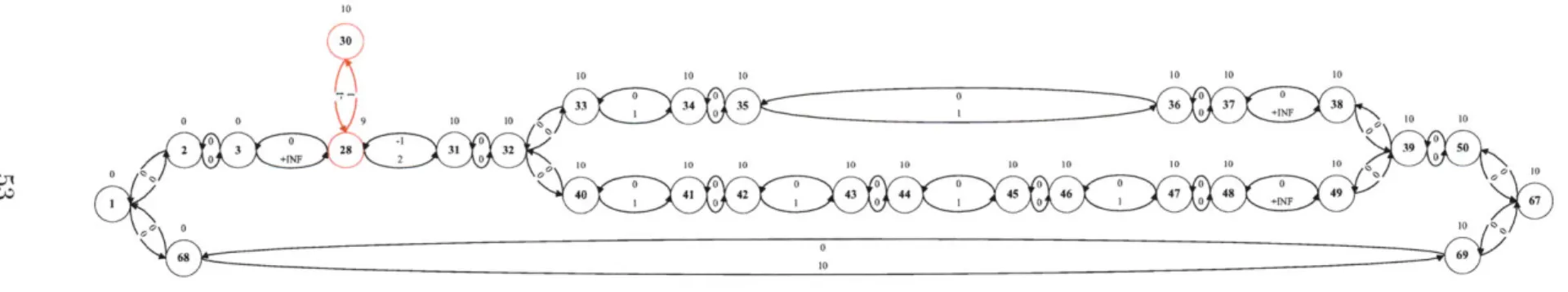
first section of the plan has been collapsed to a single simple temporal constraint. The plan contains both the sequence and parallel constructs. For example, at the highest level, the plan consists of two subnetworks in parallel; a subnetwork between nodes 2 and 50 and another between nodes 68 and 69. The upper subnetwork, between nodes

3 and 39, is a series subnetwork, consisting of three activities (nodes 3 and 27, 28

and 29, and 30 and 31) followed by a parallel subnetwork (nodes 32 to 39). Note that nodes 2 and 50 are present as the remnants of the choose subnetwork from the complete TPN, which is introduced in Section 2.4.

In order for a temporally flexible plan to be executable, it must be temporally

con-sistent. We discuss the methods used to test for temporal consistency in Section 2.5.

Definition 1 A temporally flexible plan is temporally consistent if there exists a

feasible

Definition 2 A

feasible

41

(Syn otion) WAMO.MvTHomeLao. (WMI., fo WAMI co.mplet)

[0.0) 0,(0.0] [0- ]

(Coll ton) (Syn o tonoo) WAMO.Op H..d 3 3n7d

S I [0,0] [0, 1] [0.0] [0,1] [0.0] [00]

2 3 27 28 29 30 31 32 (Syoa-tion) 0 WAM.MoveToDropffltio n WAMI.OpenHad WAMo vdr oo ocatol (W.afo WAMO0coplet) o 39 50

S[01[0,1] [0,1] [0,1] 0,0] [0,+ ] 6

40 41 42 43 4 4 pi 4... ' l 1 461 47 48 49 6

69

68 ? 69

Figure 2-2: This figure shows a simplified version of the plan from the manipulator tool delivery example used in Chapter 1 as an example of a temporally flexible plan.

an assignment of execution times to each time-point in the plan such that all temporal

constraints are satisfied.

The example plan in Fig. 2-2 is temporally consistent because none of the temporal constraints conflict. This allows the executive to assign an execution time to each node without violating any temporal constraints. For example, consider node 32 in Fig. 2-2. The maximum duration specified by all of the edges between nodes 1 and 32 is

+INF

+INF

32 to be executed at any time between times 1 and 10 and these constraints will be

satisfied. All of the nodes in the plan can be scheduled in this way, so the plan is temporally consistent.

2.3

Dispatchable Execution

Given a temporally flexible plan to be executed, traditional execution schemes select a feasible execution schedule at planning time. This approach eliminates the temporal flexibility in the plan prior to execution, which leads to two problems. First, the fixed schedule lacks the flexibility needed to respond to variation in activity durations at execution time, so the plan is prone to failure. Second, if we generate a very conser-vative schedule to increase the likelihood of successful execution, then the execution becomes sub-optimal in terms of total execution time.

This limitation can be overcome through the methods of dispatchable execu-tion [20], in which scheduling is postponed until dispatch time. This means that the plan retains temporal flexibility until it is dispatched. The dispatcher schedules events reactively, assigning execution times just-in-time using the observed execution times of previously executed events. This provides robustness to uncertain durations that lie within the temporally flexible bounds of the plan.

In traditional execution schemes, where events are scheduled at planning time, 43