A decomposition-based approach to uncertainty quantification of multicomponent systems

A Decomposition-Based Approach to Uncertainty

Quantification of Multicomponent Systems

by

Sergio Daniel Marques Amaral

B.S., Pennsylvania State University (2005)

S.M., Pennsylvania State University (2007)

Submitted to the Department of Aeronautics and Astronautics !

in partial fulfillment of the requirements for the degree of

Doctor of Philosophy

at the

MASSACHUSETTS INSTITUTE OF TECHNOLOGY

August 2015 (5Pgerebet-7a6_j

@

Massachusetts Institute of Technology 2015. All rights reserved.

Signature redacted

A uthor ...

Departm~nt f Aeronautics and Astronauti

Signature redacted

July 21, 201

C ertified by ...

...

Karen E. Willcc

Professor of Aeronautics and Astronauti

,4

Chair, Thesis Committ

Certified by...

Signature redacted

A

Sign

5

..

,e

Youssef Marzouk

ssociate Professor of Aeronautics and Astronautics

ature redacted

Member, Thesis Committee

Y . . . .

Douglas Allaire

Assistant Professor of Mechanical Engineering, Texas A&M University

Member, Thesis Committee

Accepted by ...

ignature redacted...

Paulo Lozano

Associate Professor of Xeronautics and Astronautics

C

d, b

-A Decomposition-Based -Approach to Uncertainty

Quantification of Multicomponent Systems

by

Sergio Daniel Marques Amaral

Submitted to the Department of Aeronautics and Astronautics on August 18, 2015, in partial fulfillment of the

requirements for the degree of Doctor of Philosophy

Abstract

To support effective decision making, engineers should comprehend and manage var-ious uncertainties throughout the design process. In today's modern systems, quan-tifying uncertainty can become cumbersome and computationally intractable for one individual or group to manage. This is particularly true for systems comprised of a large number of components. In many cases, these components may be developed by different groups and even run on different computational platforms, making it challenging or even impossible to achieve tight integration of the various models.

This thesis presents an approach for overcoming this challenge by establishing a divide-and-conquer methodology, inspired by the decomposition-based approaches used in multidisciplinary analysis and optimization. Specifically, this research focuses on uncertainty analysis, also known as forward propagation of uncertainties, and sen-sitivity analysis. We present an approach for decomposing the uncertainty analysis task amongst the various components comprising a feed-forward system and synthe-sizing the local uncertainty analyses into a system uncertainty analysis. Our pro-posed decomposition-based multicomponent uncertainty analysis approach is shown to converge in distribution to the traditional all-at-once Monte Carlo uncertainty analysis under certain conditions. Our decomposition-based sensitivity analysis ap-proach, which is founded on our decomposition-based uncertainty analysis algorithm, apportions the system output variance among the system inputs. The proposed decomposition-based uncertainty quantification approach is demonstrated on a mul-tidisciplinary gas turbine system and is compared to the traditional all-at-once Monte Carlo uncertainty quantification approach.

To extend the decomposition-based uncertainty quantification approach to high dimensions, this thesis proposes a novel optimization formulation to estimate statistics from a target distribution using random samples generated from a (different) proposal distribution. The proposed approach employs the well-defined and determinable em-pirical distribution function associated with the available samples. The resulting optimization problem is shown to be a single linear equality and box-constrained quadratic program and can be solved efficiently using optimization algorithms that

scale well to high dimensions. Under some conditions restricting the class of

distri-bution functions, the solution of the optimization problem yields importance weights that are shown to result in convergence in the Ll-norm of the weighted proposal empirical distribution function to the target distribution function, as the number of samples tends to infinity. Results on a variety of test cases show that the proposed approach performs well in comparison with other well-known approaches.

The proposed approaches presented herein are demonstrated on a realistic appli-cation; environmental impacts of aviation technologies and operations. The results demonstrate that the decomposition-based uncertainty quantification approach can effectively quantify the uncertainty of a multicomponent system for which the models are housed in different locations and owned by different groups.

Chair, Thesis Committee: Karen E. Willcox I

Title: Professor of Aeronautics and Astronautics Member, Thesis Committee: Youssef Marzouk

Title: Associate Professor of Aeronautics and Astronautics Member, Thesis Committee: Douglas Allaire

Acknowledgments

The work presented in this thesis would not be possible without the support of many people for whom I owe a great deal of thanks.

First and foremost, I would like to express my deepest gratitude to my advisor, Prof. Karen Willcox. I cannot begin to express in words my appreciation for accepting me as her student and providing me with this opportunity. Her guidance, encour-agement, and compassion always raised my spirits and encouraged me to progress my research further. The knowledge I have acquired under her advisement, both academically and professionally, will always resonate with me throughout my future endeavors.

I would also like to thank the members of the thesis committee, Prof. Youssef Marzouk and Prof. Douglas Allaire. Their valuable insights and technical support continuously improved the quality of my thesis. I would like to especially thank Prof. Douglas Allaire who would always lend an ear to my broad ideas and offer support. My gratitude is also extended to Prof. Qiqi Wang and Dr. Elena de la Rosa Blanco for their comments and questions on the thesis, which have also served to improve the quality.

I also have to thank the many people who provided excellent support outside of my research. To my colleagues at ACDL and LAE, thank you for sharing this experience with me. I would like to especially recognize my lab members at ACDL including Chad Lieberman, Benjamin Peherstorfer, Tiangang Cui, Daniele Bigoni, Florian Augustin, Alessio Spantini, Alex Gorodetsky, R6mi Lam, Han Chen, Xun Huan, Eric Dow, Luico Di Ciaccio, and Giulia Pantalone. I would also like to thank my lab members at LAE including Steve Yim, Akshay Ashok, Fabio Caiazzo, Chris Gilmore, and Sebastian Eastham. I would like to thank AeroAstro staff members including Jean Sofronas, Joyce Light, Beth Marois, Melanie Burliss, and Meghan Pepin - I appreciate everything you have done to make my time here that much more rewarding and manageable.

friends. Madalina Persu, Domoinik Bongartz, Sebastian Eberle, Herve Courthion, Frank Dubois, and Marcel Tucking- thank you for pulling me away from work and helping me keep things in perspective. Ryan Carley, Katherine Li, Ryan Sullivan, Kel Elkins, Ryan Surmik, and Jay Hoffman - thank you for the support, dedication, and all the laughs throughout these years. To Sari Rothrock, I can not thank you enough for helping me fulfill my dream.

Finally, I would like to thank my family for their unyielding love and support. To my brothers, John Amaral and Eric Amaral, I may have left home at a young age but not a day goes by that I do not think about the times we spent together. Thank you for your unwavering support and know that it is reciprocated. To my parents, Jodo Paulo Amaral and Beatriz Amaral, I am where I am today because of your steadfast love, guidance, and determination. Like many immigrants, they came in pursuit of better opportunities for themselves and their children. While it took me most of my youth to come to realize the scale of their sacrifice, I hope I achieved the dream you had for me, I love you.

The work presented in this thesis was funded in part by the United Stated Federal Aviation Administration Office of Environmental and Energy Award Number 09-C-NE-MIT, Amendment Numbers 028, 033, and 038, by the International Design Center at the Singapore University of Technology and Design, and by the DARPA META program through AFRL Contract Number FA8650-10-C-7083 and VU-DSR #21807-S7.

Contents

1 Introduction

1.1 Motivation for decomposition-based uncertainty quantification

1.2 D efinitions . . . .

1.3 Uncertainty analysis . . . .

1.5 Current practices for uncertainty quantification in systems . .

1.6 Thesis objectives . . . .

1.7 Thesis outline . . . .

2 Decomposition-Based Uncertainty Analysis

2.1 Introduction to decomposition-based uncertainty analysis . . .

2.2 Local uncertainty analysis . . . .

2.3 Sample weighting via importance sampling . . . . 2.4 Density estimation for estimating importance weights . . . . .

2.5 Accounting for dependency among variables . . . .

2.6 Convergence analysis & a posteriori indicator . . . . 2.6.1 Convergence theory . . . .

2.6.2 A posteriori indicator . . . .

2.6.3 Convergence example . . . .

2.7 Application to a gas turbine system . . . .

2.7.1 Gas turbine system setup . . . . 2.7.2 Uncertainty analysis . . . .

2.7.3 Flexibility of decomposition-based uncertainty analysis

27 . . . . 28 . . . . 29 . . . . 33 . . . . 35 . . . . 37 . . . . 39 . . . . 40 41 42 46 47 49 51 55 55 58 59 62 63 67 69

2.8 Pitfalls of decomposition-based uncertainty analysis

3 Decomposition-Based Global Sensitivity Analysis 3.1 Variance-based global sensitivity analysis . . . .

3.1.1 Formulation . . . .

3.1.2 Computing sensitivity indices . . . .

3.2 Decomposition-based global sensitivity analysis . . 3.2.1 Formulation . . . .

3.2.2 Algorithm . . . .

3.3 Application to a gas turbine system . . . .

3.3.1 Gas turbine system setup . . . . 3.3.2 Global sensitivity analysis . . . .

4 Optimal L2-norm empirical importance weights

4.1 Introduction to empirical change of measure . . . .

4.1.1 Definitions and Problem Setup . . . .

4.1.2 Current Practices . . . . 4.1.3 Proposed Approach . . . . 4.2 Optimization Statement . . . . 4.3 Numerical Formulation . . . . 4.3.1 Single Linear Equality and Box-Constrained

4.3.2 Karush Kuhn Tucker Conditions . . . .

4.4 Convergence . . . . 4.5 Solving the Optimization Statement . . . .

4.5.1 Analytic Solution for R . . . .

4.5.2 Optimization Algorithm . . . .

4.6 Applications . . . .

4.6.1 One-Dimensional Numerical Example . . . .

4.6.2 Importance Sampling . . . . 72 75 . . . . . 76 . . . . . 76 . . . . . 79 . . . . . 80 81 81 . . . . . 84 . . . . . 84 . . . . . 85

Quadratic

5 Environmental Impacts of Aviation

5.1 Introduction to environmental impacts of aviation'

5.2 Transport Aircraft System Optimization

5.2.1 TASOpt Inputs . . . .

5.2.2 TASOpt Outputs . . . .

5.3 Aviation Environmental Design Tool . .

5.3.1 AEDT Inputs . . . . 5.3.2 Flight Trajectories . . . . 5.4 TASOpt-AEDT Interface . . . . 5.4.1 Transformation Procedure . . . . 5.4.2 Validation . . . . 5.5 Dimension Reduction . . . . 5.5.1 Problem Setup . . . .

5.5.2 Generalized ANOVA Dimensional

5.5.3 Results . . . . 5.6 Uncertainty quantification . . . . 5.6.1 Uncertainty Analysis . . . . 129 . . . . 130 Decomposition

5.6.2 Global Sensitivity Analysis . . . .

6 Conclusions

6.1 Sum m ary . . . .

6.2 Future work . . . .

A TASOpt Random Input Variables

B AEDT Random Input Variables

132 132 133 135 135 135 137 137 139 141 142 144 146 147 148 150 153 153 156 159 161

List of Figures

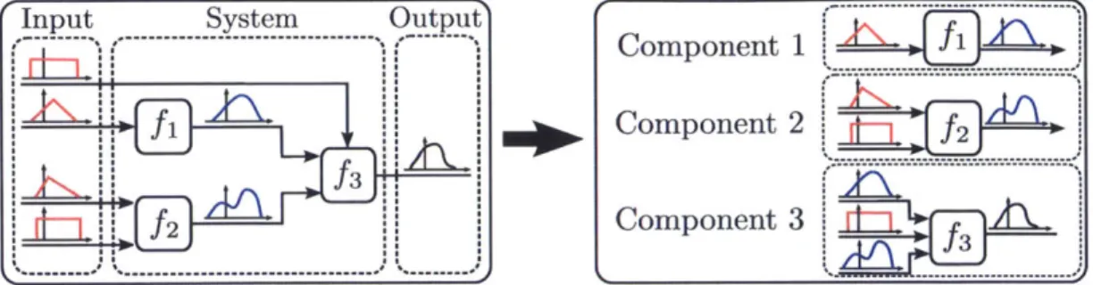
1-1 The feed-forward multicomponent system presented here illustrates how

uncer-tainty in the inputs propagate throughout the system and ultimately to the system

outputs. Different architectures of feed-forward multicomponent systems may also

be represented with a similar diagram. . . . . 30

2-1 The proposed method of multicomponent uncertainty analysis decomposes the

problem into manageable components, similar to decomposition-based approaches used in multidisciplinary analysis and optimization, and synthesizes the system

uncertainty analysis without needing to evaluate the system in its entirety. . . . 42

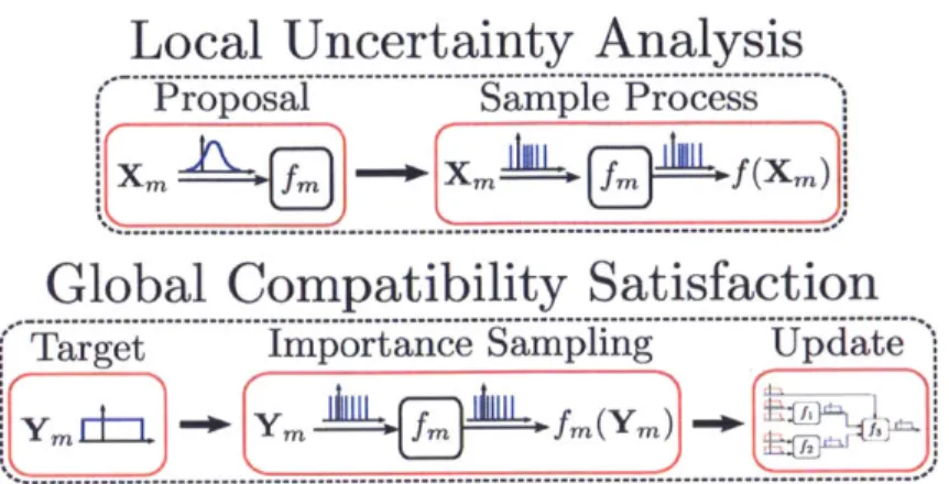
2-2 The process depicts the local uncertainty analysis and global compatibility

sat-isfaction for component m. First, local uncertainty analysis is performed on the component. Second, global compatibility satisfaction uses importance sampling to update the proposal samples so as to approximate the target distribution. Finally,

an update step accounts for dependency among variables. . . . .. . . . 43

2-3 Three components of a feed-forward system shown from the system Monte Carlo

perspective (left) along with the same components exercised concurrently from the perspective of the decomposition-based multicomponent uncertainty analysis (right). 45

2-4 The importance sampling process uses the realizations (red dots on left figure)

generated from a proposal distribution Px( 1, 2) (corresponding density shown as

red solid contour on left figure) to approximate a target distribution Py (1, )

(blue dash contour on left figure), by weighting the proposal realizations, (blue

2-5 The results indicate the output of interest, 6, Cramer von-Mises criterion converges with the number of samples. The system Monte Carlo weighted empirical distri-bution function uses w = 1,T. The decomposition-based multicomponent weighted

empirical distribution function uses weights computed via Algorithm 1. . . . . . 62

2-6 The results show the implications of selecting a poor proposal distribution for

component f2 with n = 256. As neff approaches n, indicating a better proposal

distribution, the accuracy of our estimate improves. . . . . 63

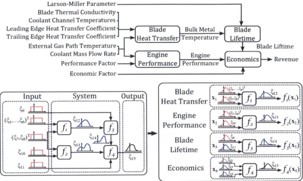
2-7 The gas turbine application problem contains four components, each representing a disciplinary analysis: heat transfer, structures, perfor-mance, and economics. . . . . 64

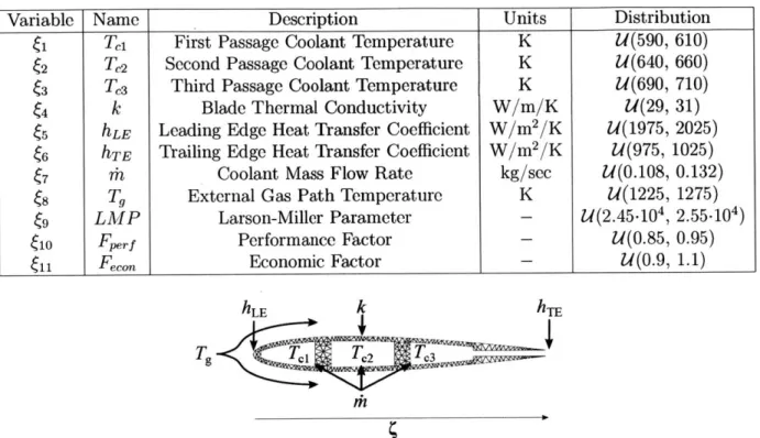
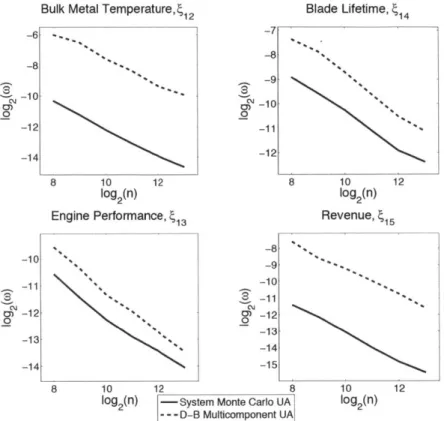
2-8 The gas turbine blade profile and mesh, along with the random input variables. . . . . 65 2-9 The Cramer von-Mises convergence plots are shown for the

intermedi-ate variables $2, $13, and $1 as well as for the system output of

inter-est, revenue, $15. The solid lines are the result obtained from a system Monte Carlo simulation. The dashed lines are the result obtained using our decomposition-based multicomponent uncertainty analysis. ... 69

2-10 The system output of interest, revenue, distribution function using n = 8192 samples is shown in millions of dollars. The solid line is the

result obtained from a system Monte Carlo simulation. The dashed line is the result obtained from the decomposition-based multicomponent uncertainty analysis. The dash-dot line is the result obtained from the local uncertainty analysis of the Economics model . . . . . 70

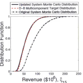
2-11 The system output of interest, revenue, distribution function using

n = 8192 samples is shown in millions of dollars. The solid line is

the result obtained from an updated system Monte Carlo simulation which required evaluating the entire system again. The dashed line is the result obtained from the decomposition-based multicomponent uncertainty analysis using the online phase only. The dash-dot line is the result from the previous Monte Carlo uncertainty analysis. ... 71

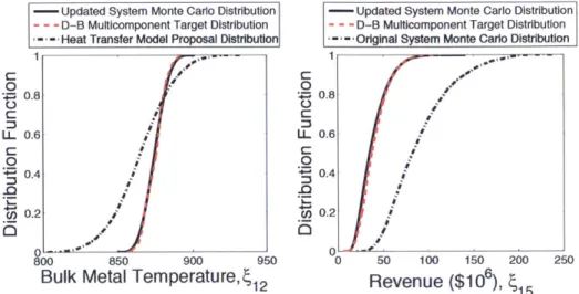
2-12 The bulk metal temperature, 12, is shown on the left. The results shows that the proposal distribution (dash-dot line) of the bulk metal temperature of the Lifetime model supports the target distribution (dashed line) coming from the Heat Transfer model. The system Monte Carlo uncertainty analysis results, solid line, required evalu-ating the the Heat Transfer, Lifetime, and Economics model, whereas the decomposition-based multicomponent uncertainty analysis results were obtained using the online phase only. The revenue, 15, in millions

of dollars is shown on the right. The solid line is the result obtained from a system Monte Carlo uncertainty analysis. The dashed line is the result obtained from the decomposition-based multicomponent un-certainty analysis using the online phase only. The dash-dot line is the result obtained from the previous Monte Carlo uncertainty analysis. . 72

3-1 The proposed method for multicomponent global sensitivity analysis utilizes the

decomposition-based uncertainty analysis algorithm presented in Chapter 2 to eval-uate the statistics of interest necessary for the variance-based method of I.M. Sobol'. The objective of a variance-based global sensitivity analysis method is to apportion the output of interest variance across the system inputs and is depicted here using

the pie chart. . . . . 76

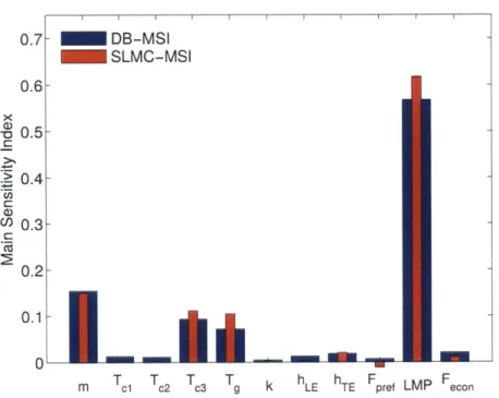
3-2 The decomposition-based main effect indices (DB-MSI) are plotted against the

all-at-once Monte Carlo main effect indices (SLMC-MSI). The results demonstrate that the decomposition-based approach quantifies the main effect indices accurately

3-3 The decomposition-based main effect indices (DB-MSI) are plotted against the all-at-once Monte Carlo main sensitivity indices (SLMC-MSI). The plot on the (left)

implements K = 2 partitions and n = 10, 000 proposal samples. The plot on

the (right) implements K = 2 partitions and n = 5,000 proposal samples. These

results show two scenarios for which the decomposition-based global sensitivity analysis algorithm performs inadequately. On the (left) our approach suggests the sum of the main effect indices are greater than unity. On the (right) our approach

erroneously suggests T,2 is an influential system input. . . . . 87

4-1 The proposed approach minimizes, with respect to empirical impor-tance weights associated with the proposal random samples, the L2

-norm between the weighted proposal empirical distribution function and the target distribution function. In this example, we generated n = 100 random samples from the proposal uniform distribution

func-tion, U(0, 1). The results show our weighted proposal empirical distri-bution function, labeled "L20 Weighted Proposal", accurately repre-sents the target beta distribution function, B(0.5,0.5). . . . . 93

4-2 Performance of our optimal empirical importance weights determined using the Frank-Wolfe algorithm with step length a = 2/(2 + k) and premature termination. This example uses n = 100 proposal random

samples generated from a uniform distribution function, U(0, 1). The target distribution function is the beta distribution function, B(0.5, 0.5). Terminating the Frank-Wolfe algorithm after 25 iterations (top) re-sults in a sparse empirical importance weight vector. Terminating the Frank-Wolfe algorithm after 100 iterations (bottom) results in a dense solution and as a result a more accurate representation of the target distribution function. . . . . 115

4-3 Discrepancy reduction for d = 2. Both algorithms reduce the L2-norm discrepancy (i.e., r < 1) in both scenarios. The Frank-Wolfe algorithm converges more quickly than the Dai-Fletcher algorithm. . . . . 124

4-4 Discrepancy reduction for d = 5. Both algorithms reduce the L2-norm discrepancy (i.e., r < 1) in both scenarios. The Frank-Wolfe algorithm

converges more quickly than the Dai-Fletcher algorithm, although the final results are similar. . . . . 125

4-5 Discrepancy reduction for d = 10. Both algorithms reduce the L2

-norm discrepancy (i.e., r < 1) in both scenarios. The Dai-Fletcher

algorithm converges more quickly the Frank-Wolfe algorithm, although the final results are similar. . . . . 126

4-6 Discrepancy reduction for d = 5 and a large number of samples. The

Frank-Wolfe algorithm reduces the L2-norm discrepancy (i.e., r < 1) in both scenarios for a large-scale application problem (i.e., large n). The results presented are the average over 100 simulations. . . . . 127

5-1 System-level uncertainty quantification of the toolset consists of quan-tifying how uncertainty in aircraft technologies and operations impact the uncertainty in the outputs of interest, here the aircrafts fuel con-sumption performance. The descriptions for the TASOpt input

vari-ables and AEDT input varivari-ables are provided in Appendix A and

Ap-pendix B, respectively. . . . . 131

5-2 Boeing 737-800W airframe configuration. Schematic taken from [26]. 132

5-3 Illustrated here are the 20 representative flight trajectories flown by

the Boeing 737-800W in the TASOpt-AEDT uncertainty quantification

study. ... . ... .. . .. . . ... . . . . .. . .. . .. . 137

5-4 Validation study of the TASOpt component to AEDT component

trans-formation for the Boston to Atlanta great circle flight. The results il-lustrate that the fuel burn rate (FBR) and net corrected thrust (NCT) match well throughout most of the flight trajectory. . . . . 140

5-5 We partitioned the AEDT input variables into two sets; an influential set and a noninfluential set. The distribution function of the AEDT inputs in the second set are not required to converge weakly to the target distribution function. . . . . 143

5-6 This plot presents the absolute variance- and covariance-driven sen-sitivity indices from each of the 50 AEDT random input variables on the AEDT fuel consumption performance variance. This plot il-lustrates that the absolute variance- and covariance-driven sensitivity indices decays very rapidly and that 15 AEDT random input variables capture almost all of the AEDT fuel consumption performance variance. 147

5-7 Sensitivity matrix of the 15 most influential AEDT random input vari-ables impacting the AEDT fuel consumption performance variance. . 148

5-8 We partitioned the AEDT input variables into two sets; an influential set and a noninfluential set. The noninfluential set contains AEDT in-put variables which were deemed not to influence the cruise and takeoff segments as well as input variables which were labeled as noninfluential

by the AEDT component global sensitivity analysis. The influential

set contains AEDT random input variables which were labeled as in-fluential by the AEDT component global sensitivity analysis. . . . . . 149

5-9 The AEDT fuel consumption performance distribution is shown here using the AEDT output proposal distribution, all-at-once Monte Carlo uncertainty analysis, and the decomposition-based uncertainty analy-sis. These results suggest that our decomposition-based uncertainty analysis performed adequately which implies the change of measure across the 15 AEDT random input variables was successful and that the correct 15 AEDT random input variables were selected by the

5-10 The AEDT fuel consumption performance probability density

func-tion is shown here using the AEDT output proposal probability den-sity function, all-at-once Monte Carlo uncertainty analysis, and the decomposition-based uncertainty analysis. These results complement the distribution function results provided in Figure 5-9 and suggest that our decomposition-based uncertainty analysis performed adequately which implies the change of measure across the 15 AEDT random input variables was successful and that the correct 15 AEDT random input variables were selected by the AEDT component-level global sensitivity analysis. . . . . . . . . 151 5-11 The system-level main sensitivity indices are shown here using the

all-at-once Monte Carlo global sensitivity analysis and the

based global sensitivity analysis. These results suggest that our decomposition-based global sensitivity analysis performed adequately and that only a

handful of technological and operational system input variables have a significant influence, on average, on the system output of interest. A description of the system inputs are provided in Appendix A . . . . . 152

List of Tables

2.1 Index sets for the system presented in Figure 2-3. . . . .

2.2 Gas turbine system input uncertainty distributions where U(a, b) rep-resents a uniform distribution between the lower limit a and upper

lim it b. . . . .. . . . . .. . . . . .. . . . .

2.3 Heat transfer model input proposal uncertainty distributions. ...

2.4 Blade lifetime model input proposal uncertainty distributions...

2.5 Performance model input proposal uncertainty distributions. . . . . .

2.6 Economics model.input proposal uncertainty distributions. . . . .

2.7 Updated gas turbine system input uncertainty distributions. . . . . .

3.1 The performance of the decomposition-based global sensitivity analysis

algorithm as quantified by Equation 3.22 is presented. The results

sug-gest the decomposition-based global sensitivity analysis degrades with decreasing number of partitions and decreasing number of proposal sam ples. . . . . 52 65 66 66 67

67

70

87

4.1 The error metric rn, Equation (4.58), measured as a percentage, for the four methods and all four scenarios. Results are averaged over 100 independent trials and the term in parentheses is the corresponding standard deviation. Bold text indicates the best estimate for all the methods not including importance sampling (IS). The importance sam-pling results use the unknown proposal and target probability density functions to define the density ratio. The importance sampling results are provided here in order to compare to the standard solution using the unknown probability density functions. The results demonstrate that the proposed approach (L20) outperforms the previous approaches. The proposed approach degrades with increasing dimensions and de-creasing number of proposal and target random samples, however, less so than the other approaches. ... ... 119

4.2 The ratio of discrepancy computed using our optimal empirical impor-tance weights and uniform imporimpor-tance weights, Equation (4.61) mea-sured as a percentage. Shown are results for the d = 1 case, averaged over 100 independent trials. The term in parentheses is the

correspond-ing standard deviation. n is the number of proposal random samples. 122

5.1 TASOpt random input variables and their respective distributions. . . 133 5.2 The performance of each sampled aircraft configuration is evaluated

using a Latin hypercube design of experiments. Presented here are the TASOpt mission input variables and their respective uniform distribu-tion parameters (i.e., U(a, b)). Parameters containing an asterisk are also TASOpt random input variables. Therefore, the parameters rep-resent differences from their respective realization (i.e., U(x - a, x + b)

where x is the variables sample realization). . . . . 134

5.3 Presented here are the 20 representative flight trajectories (i.e., depar-ture, arrival, and range) flown by the Boeing 737-800W in the

5.4 Presented here are the fuel consumption results over the three flight trajectories. The TASOpt row represents an aircraft generated by and flown in TASOpt. The AEDT row represents the TASOpt air-craft imported into the AEDT component through the component-to-component transformation and then flown on the same flight trajectory as the TASOpt flight trajectory. . . . . 141

Nomenclature

d Number of system variables

dn, Number of inputs to Component m

fm

h Radon-Nikodym importance weight

k~m Number of outputs of Component m

neff Effective sample size

Px Proposal density function

py Target density function

t Integration variable

w Importance sampling weights

W; L2-norm optimal importance sampling weights

Xi ith component of the vector x

x Vector of system variables

XAmt Vector of variables with indices in the set Am X.7J Vector of variables with indices in the set 1m xJm _{Vector of variables with indices in the set Jn} X/m Vector of variables with indices in the set ICm XOm Vector of variables with indices in the set 0,m, XSm Vector of variables with indices in the set Sm

XTm Vector of variables with indices in the set 'T

XUm Vector of variables with indices in the set Urn

Yi Vector of inputs to Component m

6 Equality constraint Lagrange multiplier

A Inequality constraint Lagrange multiplier

it Proposal measure

v Target measure

Ti Total sensitivity index of the ith input

W L2-norm distance metric between two distribution functions

IP Probability measure

X Random variable associated with measure p

Y Random variable associated with measure v Ym Random vector of inputs to Component m

D Variance

DA Variance associated with the set A

D2 L2-norm discrepancy metric

K Kernel function

L Bandwidth parameter in kernel density estimation

M Number of Components which compose the system

Px Proposal distribution function

P Proposal empirical distribution function

PZW Proposal importance weighted empirical distribution function

Py Target distribution function

PV Target empirical distribution function

SA Sensitivity index of set A

Amn Set of indices of the system variables that are a subset of inputs to Component m B(a, b) Beta distribution with parameters a and b

'Dm Domain of integration for Component m

F a-algebra

IM Set of indices of the system variables that are inputs to Component m

Jm Set of indices of all of the inputs and outputs associated with the first m - 1

Km

Set of indices in

with the exception of those indices in 1,

Mi ith set of components

KJ(p,

E)

Gaussian distribution with mean p and covariance E

L

Lagrangian

Om

Set of indices of the outputs of Component m

Pk Set parition [tk, tk+1)

Sm

Set of indices of new system inputs to Component m

TM

Set of indices of the shared inputs of Component m with any of the previous m

-

1

components' inputs or outputs

UM

Set of indices of the inputs and outputs of the first m components

U(a, b)

Uniform distribution between a and b where a < b

Vm

Set of indices of the inputs and outputs of Component m

Q

Sample space

HI

Generic distribution function

7r Generic density function

r

Estimate of a density function,

I

Indicator function

1Vector of size n containing entires equal to 1

Chapter 1

Introduction

To support effective decision making, engineers should characterize and manage vari-ous uncertainties throughout the design process. Herein, the science of characterizing and managing uncertainties throughout the design process is referred to as uncer-tainty quantification [781. Although uncertainty quantification is known to encom-pass a large scope [109], this research will focus on uncertainty analysis, also known as forward propagation of uncertainties, and sensitivity analysis. In today's modern systems, quantifying uncertainty can become cumbersome and computationally in-tractable for one individual or group to manage. This is particularly true for systems comprised of a large number of components. In many cases, these components may be developed by different groups and even run on different computational platforms. Recognizing the challenge of quantifying uncertainty in multicomponent systems, we

establish a divide-and-conquer approach, inspired by the decomposition-based

ap-proaches used in multidisciplinary analysis and optimization [19, 64, 110, 61].

Motivation for uncertainty quantification of multicomponent systems is given in Section 1.1. In Section 1.2, the notation for subsequent developments and the problem statement are presented. The current practices in uncertainty analysis and sensitivity analysis for a single component are discussed in Section 1.3 and Section 1.4 respec-tively. The current practices in uncertainty quantification of multicomponent systems are discussed in Section 1.5. The objectives of this research are stated in Section 1.6,

1.1

Motivation for decomposition-based uncertainty

quantification

Multidisciplinary analysis is an extensive area of research, intended to support today's modern engineered systems which are designed and developed by multiple teams. In addition to the difficulties associated with the design of such systems, the need to enhance performance and efficiency often drives the design to its physical limits. Therefore, the current methodology of modeling a baseline scenario and taking into account safety factors may no longer be sufficient. Instead, a rigorous characterization and management of uncertainty is needed, using quantitative estimates of uncertainty to calculate relevant statistics and failure probabilities. To estimate relevant statistics and failure probabilities requires an uncertainty quantification of the entire system. However, uncertainty quantification of the entire system may be cumbersome due to factors that result in inadequate integration of engineering disciplines, subsystems, and parts, which we refer to collectively here as components. Such factors include components managed by different groups, component design tools or groups housed in different locations, component analyses that run on different platforms, components with significant differences in analysis run times, lack of shared expertise amongst groups, and the sheer number of components comprising the system.

Here we present some real world examples illustrating the challenges and out-comes of designing today's modern engineered systems. Boeing's latest aircraft, the Boeing 787 "Dreamliner", is an example of a complex system that has been afflicted with unanticipated costs and delays due to system engineering errors [105, 37]. Gen-eral Motors electric vehicle, the Chevy Volt, has also seen its assembly cost inflate to double the initial estimate [1191. NASA's International Space Station and the Constellation programs each experienced schedule delays and cost overruns due to factors such as organizational and technical issues [4]. These real world examples illustrate how our current design methodologies may no longer be adequate to ana-lyze systems which have become increasingly complex and, therefore, progressively more difficult to design and manage. By characterizing and managing uncertainty

in complex systems, such as those presented, we can provide relevant statistics such as the probability of a schedule delay or cost overrun to further support decision-and policy-making processes. Government agencies, having acknowledged the impor-tance of uncertainty quantification in design, have taken up the challenge to address these problems by launching new research initiatives in complex systems design under uncertainty [28, 107].

More specifically, in a National Science Foundation workshop on multidisciplinary design and optimization for complex engineered systems; dealing with uncertainty was listed as an overarching theme for future research [1071. The workshop also emphasized the importance of keeping humans in the loop. In the report, it was stressed that a team was necessary, due to the fact that people invariably specialize in a single discipline and must, therefore, work as a team to achieve multidisciplinary objectives. Given today's engineered systems are so complex that they are beyond the comprehension of a single engineer, even design convergence can become an issue depending on how the team is organized. These challenges are only heightened by the fact that globalization has spread the design of the complex engineered system across the world. These observations suggest there is a lacking but necessary aspect of system engineering and design that this research addresses, decomposition-based uncertainty quantification of multicomponent systems. The proposed approach de-composes the multicomponent uncertainty quantification task amongst the various components comprising the multicomponent system and synthesizes these local anal-yses to quantify the uncertainty of the multicomponent system.

1.2

Definitions

Multicomponent system

Illustrated in Figure 1-1 is a feed-forward multicomponent system whereby uncer-tainty in the system inputs are propagated throughout the system and ultimately to the system output. Here we formally define the feed-forward multicomponent sys-tem along with its respective components and introduce the notation required for

Figure 1-1: The feed-forward multicomponent system presented here illustrates how uncertainty in the inputs propagate throughout the system and ultimately to the system outputs. Different ar-chitectures of feed-forward multicomponent systems may also be represented with a similar diagram.

subsequent developments. We take this opportunity to discuss any assumptions and limitations imposed on our feed-forward multicomponent system.

Definition 1. A system is a collection of M coupled components. Each component

has an associated function that maps component input random variables to component output random variables. Let x [x1, x2,... ,Xd]T be the vector of system variables, comprised of the inputs and outputs of each component of the system, where shared inputs are not repeated in the vector. For component m, where m E {1, 2, ... , M},

let ZE C {1, 2,... , d} denote the set of indices of the system variables

correspond-ing to inputs to component m and let O, C {1, 2,. .., d} denote the set of indices

corresponding to the outputs from component m. Define dn = 1nI and k, = |rn. We denote the function corresponding to component m as f. : Rd- -+ Rkm, which

maps that component's random input vector, Xy. : Q -+ d₁ , where Q is the prod-uct sample space of the input random vector, into that component's random output vector, Xom = f,,(X1.). A system whose components can be labeled such that the

inputs to the it" component can be outputs from the jth component only if j < i is a feed-forward system.

Additionally, for each component function, fn, there exists sets {I1, 12,..., I, }

that partition the component input space Rdm, such that fm : I --+ Rk. is strictly

one-to-one and continuously differentiable for each i E

{1,

}.

Input System Output

with the complementary set A

=

Im\ Am and cardinality 0 <

IAm|

I

d

and let

XAm

: Q -+

be a subset of Xm with

defining the complementary subset.

Probability framework

Let t

E

Rd be a generic point and designate entries of t by subscript notation as

follows t = [ti, t2,... , td]T. Let (Q,F, P) be a probability space, where Q is a sample

space, T is a c--field, and P is a probability measure on (Q,7). Then the random

variable Y : Q - Rd is associated with the continuous measure v on Rd, such that

v(A) =

P(Y-'(A)) for

E

Define

and py(t) to be the distribution function

and probability density function of Y evaluated at t, respectively. The distribution

function and probability density function are defined as

Py(t)

=

v((-oo, t]),

(1.1)

and

py(t) -

dPy(t)

dx

respectively. Likewise, the random variable X : Q

Rd

is associated with the

mea-sure p on

such that p(A)

P(X-'(A)) for

E

Similarly, define Px(t) and

px(t) to be the distribution function and probability density function of X evaluated

at t, respectively. In addition, we confine the measure v to be absolutely continuous

with respect to measure p.

Definition 2. The measure v is said to be absolutely continuous with respect to

measure p if p(A) = 0 implies v(A) = 0 for all finite sets A E Rd

/141.

In Chapter 3 we constrain the measures to have finite support.

Definition 3. A measure is said to have finite support if its support, supp(p) = {A E

Rd

I

This research does not account for discrete distributions (e.g., probability mass

func-tions) since the absolute continuity condition would require that all proposal random

samples be positioned exactly according to the target random samples. To satisfy this condition would require that we know the target distribution function for all system variables prior to performing the uncertainty quantification. However, hav-ing knowledge of the target distribution function prior to performhav-ing the uncertainty quantification nullifies our decomposition-based approach. For this reason we only consider continuous distribution functions throughout this research.

For a given 0 4 A C {1,..., d}, the marginal density function of XA is given

by pX(tA) = fRd-AI pxA(t)dtAc. Let (Q',F') be a measurable space such that the

component mapping

f

defines an output measure pf- on F' by

pf -1(A') = p(f -A'), A' E

F',

where

f-

_f,

Upon completing the uncertainty analysis, we may evaluate statistics of interest such as the moments of a quantity of interest or the probability of an event. The mean of a quantity of interest, g, is given by

Ex[g] =

j

The variance of the quantity of interest, g, is given by

varx(g) =

d

Lastly, the probability of an event A (e.g., A = {t E Rd

I

where U(t E A) is the indicator function,

1, ift

EA

0, otherwise.

1.3

Uncertainty analysis

Computational methods for uncertainty analysis of a single component can be clas-sified into two groups: intrusive and nonintrusive approaches. Intrusive approaches, also known as embedded projection approaches, introduce a solution expansion into the formulation of the stochastic problem and projects the resulting stochastic equa-tion onto the expansion basis to yield a set of equaequa-tions that the expansion coefficients must satisfy. The assembly and solution of this stochastic problem requires access and modification to the existing computational model, which may not always be available

[44, 115, 80, 68, 126, 48]. Nonintrusive approaches, also known as sampling-based

methods, do not require modification of existing computational components and in-stead treat the components as a "black-box". This research focuses on nonintrusive approaches due to their broader applicability; that is, they can be applied to a wide range of models without requiring knowledge of or access to the underlying

imple-mentation details. Within the category of nonintrusive approaches exists a collection of sampling-based methods for the forward propagation of uncertainties. We list here

the common sampling-based methods for a single component.

Monte Carlo simulation: Given the function g : Rd -+ R, that takes random inputssi uati ,d]T', we can estimate the mean ofg((1, 2,... , d) using Monte

Carlo simulation as

n = 9(C, ,

, ),(1.8)

where {{, 2.,... , } is the ith sample realization of the random input to the function. By the strong law of large numbers, g 2-+ Et[g( 1, 2,... , J)] as

n -+ oc _{[141. We may use Monte Carlo simulation to estimate other integral} quantities, such as the variance, as well, with almost sure convergence

guaran-teed by the strong law of large numbers.

Full factorial numerical integration: With this approach, the statistical moments of the quantity of interest are calculated through a direct numerical integration using an appropriate quadrature rule [3, 39]. In numerical analysis, a quadrature rule is an approximation of the definite integral of a function, usually expressed as a weighted sum of function values at specified points in the domain of inte-gration.

Projection Methods: With this approach, we express the function via orthogo-nal polynomials of the input random parameters [44, 68, 126, 48, 1251. The deterministic coefficients associated with each term of the expansion are evalu-ated through a (multivariate) integration scheme; via Monte Carlo simulation or quadrature rule.

Interpolatory Collocation Methods: With this approach, we express the func-tion as a numerical surrogate model by interpolating between a set of solufunc-tions

to the computational model [68, 126, 48, 43, 11, 127, 10, 871.

Other nonintrusive approaches not presented in detail here are expansion-based methods [118, 441, most probable point-based methods [52, 411, and nonprobabilistic-based methods [5, 82, 831. Of the sampling-nonprobabilistic-based methods available, we focus on Monte Carlo simulation. Monte Carlo simulation offers an approach which can more easily cope with dependent component inputs and high dimensional number of random inputs. Additionally, by an application of Skorokhod's representation theorem (see,

e.g., Ref. [49]), the estimated mean and variance of any quantities of interest, if they

exist, are guaranteed to converge to the true mean and variance.

To evaluate the performance of our decomposition-based multicomponent tainty analysis we will evaluate the full system uncertainty analysis. For the uncer-tainty analysis of a multicomponent feed-forward system, Monte Carlo simulation propagates uncertainty through the system's components by propagating realizations of the random inputs to the system in a serial manner. That is, realizations are

propagated through the system on a component-by-component basis, requiring com-ponents with outputs that are inputs to downstream comcom-ponents to be run prior to running downstream components. This can be problematic if components are housed in different locations or owned by different groups, due to communication challenges and the possible transfer of large datasets. Furthermore, any changes to upstream components (e.g., modeling changes, changes in input uncertainty distributions, etc.) will require recomputing all downstream uncertainty analyses.

1.4

Sensitivity analysis

Sensitivity analysis investigates the relationship between inputs and output. More-over, it allows us to identify how the variability in an output quantity of interest is related to an input in the model and which input sources dominate the response of the system. Sensitivity analysis can be categorized as local or global. A local sensitivity analysis addresses sensitivity relative to point estimates of an input value and is quantified using derivatives of the computational model evaluated at the input value. A global sensitivity analysis quantifies sensitivity with regards to the input distribution rather than a point value. In this research we focus on global sensitiv-ity analysis since we are interested in how the system behaves with respect to the system input distributions. We list here the common approaches to evaluate global sensitivity analysis of a single component.

Screening methods: This class of methods consist of evaluating the local sensitivity analysis whereby each input is varied "one-at-a-time". The sensitivity measures proposed in the original work of Morris are based on what is called an elementary effect 1841. The most appealing property of the screening methods is their low computational costs (i.e. a low required number of computational model evaluations). A drawback of this feature is that the sensitivity measure is only qualitative. It is qualitative in the sense that the input factors are ranked in order of importance, but they are not quantified on how much a given factor is

more important than others. Such methods include Morris's

One-factor-At-a-Time.

Sampling-based methods: This class of methods utilize Monte Carlo simulation

to investigate the input-output-relationship. These methods include graphical methods [131, regression analysis [55, 35], and correlation coefficients 155]. Un-like screening methods, which vary one-factor-at-a-time, these methods vary all inputs over their entire range.

Moment-independent importance measures: These methods evaluate the

in-fluence of the input uncertainty on the entire output distribution without ref-erence to any specific moment of the model output. Moment-independent im-portance measures evaluate the influence the input has on the output using a distance metric on the output probability density function or output cumulative

distribution function [25, 16, 17].

Variance-based methods: These methods quantify the amount of variance that each input factor contributes to the unconditional variance of the output. Variance-based methods offer an approach which captures the influence of the full range of variation of each input factor and the interaction effects among input fac-tors. These methods include Sobol' indices [113], high dimensional model rep-resentation [114], Jansen winding stairs [201, and Fourier amplitude sensitivity test [102].

Of the global sensitivity analysis methods available, we will focus on

variance-based methods. We perform the global sensitivity analysis using variance-variance-based meth-ods because these methmeth-ods are well-studied, are easily interpreted, and are commonly used in practice. In this research we assume the multicomponent system inputs are in-dependent. The motivation for the system-level global sensitivity analysis is research prioritization; which factor is the most deserving of further analysis or measurement?

1.5

Current practices for uncertainty quantification

in systems

Uncertainty Analysis

The challenges of system uncertainty analysis, illustrated on the left in Figure 1-1,

of-ten lie in integrating the components and in the computational expense of simulating the full system. Past work has tackled these challenges through the use of surrogate modeling and/or a simplified representation of system uncertainty. Using surrogates in place of the higher fidelity components in the system provides computational gains and also simplifies the task of integrating components [771. Using a simplified un-certainty representation (e.g., using mean and variance in place of full distributional information) avoids the need to propagate uncertainty from one component to an-other. Such simplifications are commonly used in uncertainty-based multidisciplinary design optimization methods as a way to avoid a system-level uncertainty analysis (see e.g., [1291 for a review of these methods and their engineering applications). Such

methods include implicit uncertainty propagation [501, reliability-based design

opti-mization [24], moment matching [81], advanced mean value method [62], collaborative reliability analysis using most probable point estimation [38], and a multidisciplinary

first-order reliability method [75].

Recent methods have exploited the structure of the multicomponent system to manage the complexity of the system uncertainty analysis. A likelihood-based ap-proach has been proposed to decouple feedback loops, thus reducing the problem to a feed-forward system [1041. Dimension reduction and measure transformation to reduce the dimensionality and propagate the coupling variables between coupled components have been performed in a coupled feedback problem with polynomial

chaos expansions [7, 8, 91. Multiple models coupled together through a handful of

scalars, which are represented using truncated Karhunen-Lobve expansions, have been

studied for multiphysics systems 1271. A hybrid method that combines Monte Carlo

proposed [6, 22]. The hybrid approach partitions the coupled problem into subsidiary subproblems which use Monte Carlo sampling methods if the subproblem depends on a very large number of uncertain parameters and spectral methods if the subprob-lem depends on only a small or moderate number of uncertain parameters. Another method solved an encapsulation problem, without any probability information; upon acquiring probabilistic information, solution statistics of the epistemic variables were evaluated at the post-processing steps [59, 23]. However, all the approaches presented in this review still require evaluating the system in its entirety. Since the approaches presented here do not allow for decomposing the system uncertainty quantification, these approaches do not take advantage of the decomposition-based benefits previ-ously stated in Section 1.1.

Sensitivity Analysis

As was the case in system uncertainty analysis, previous works have simplified the system through the use of surrogate modeling and/or a simplified representation of system uncertainty to perform the system sensitivity analysis. In fact, methods for the forward propagation of uncertainty in systems can be implemented to evaluate the quantities of interest required by the system sensitivity analysis. However, performing a decomposition-based sensitivity analysis of a multicomponent system raises several challenging issues which we address in Chapter 3.

Past works have tackled decomposition-based sensitivity analysis in the applica-tion of feed-forward systems. A top-down (i.e., all system variables are independent) sensitivity analysis strategy was developed to determine critical components in the system and used a simplified formulation to evaluate the main sensitivity indices

1130]. However, this approach can only be used for designing multicomponent

sys-tems with independent components (i.e., no shared variables as inputs to multiple components). To overcome the aforementioned limitations, an extended feed-forward sensitivity analysis method, was developed [74].

In the extended feed-forward sensitivity analysis method, two cases were investi-gated, dependent on whether there is a linear or nonlinear relation between upstream

component outputs and downstream component dependent coupling variables. In the case of dependent input variables, the Sobol' method has to be performed on all the independent variables and on an artificial subset variable which includes all the dependent coupling variables. Then, the covariance of the dependent coupling variables are required to compute the global sensitivity main effect indices. Lastly, in case of nonlinear dependency, a correction coefficient is used to compute the global sensitivity main effect indices. The extended feed-forward sensitivity analysis method is limited to the estimation of the main effect of the entire system and further efforts are necessary to extend this methodology for interaction effect terms. Our approach, presented in Chapter 3, avoids working with the correlation between system vari-ables and instead evaluates the necessary statistics of interest required for the system sensitivity analysis in a decomposition-based manner.

1.6

Thesis objectives

Based on the motivation and past literature works, there is a need for an uncertainty quantification methodology to manage uncertainty in the complex settings of today's modern engineered systems. This research proposes a decomposition-based vision of the multicomponent uncertainty quantification task, performing uncertainty quantifi-cation on the respective components individually, and assembling the component-level uncertainty quantifications to quantify the system uncertainty. We propose a rigor-ous methodology with guarantees of convergence in distribution. Our decomposition-based approach is inspired by decomposition-decomposition-based multidisciplinary optimization methods [19, 64, 110, 61]. This research specifically considers the problem of quan-tifying uncertainty through a feed-forward multicomponent system. To summarize, the high level objectives of this thesis are:

9 to develop a decomposition-based uncertainty analysis methodology for

feed-forward multicomponent systems with rigorous guarantees of convergence in distribution,

* to develop a decomposition-based global sensitivity analysis methodology for feed-forward multicomponent systems, and

9 to demonstrate the decomposition-based uncertainty quantification

methodolo-gies on a real world application problem.

1.7

Thesis outline

The remainder of the thesis is organized as follows. In Chapter 2, we develop the decomposition-based uncertainty analysis algorithm and discuss its technical ele-ments. We show that the decomposition-based uncertainty analysis algorithm is provably convergent in distribution and provide an illustrative example. In Chap-ter 3, we extend the ideas of ChapChap-ter 2 to develop a decomposition-based sensitivity analysis algorithm. We demonstrate the decomposition-based sensitivity analysis al-gorithm on the illustrate example presented in Chapter 2. In Chapter 4, we present an approach to change of measure which overcomes the high dimensional challenges we encounter in Chapter 2. We show that our new change of measure process, un-der moun-derate assumptions, is provably convergent in distribution. In Chapter 5, we apply the algorithms developed in this research on a real world application prob-lem; environmental impact of aviation. Additionally, we examine how an individual component-level global sensitivity analysis can be integrated into the decomposition-based multicomponent uncertainty quantification process. Finally, we summarize the thesis contributions in Chapter 6.