Econometric modeling of recycled copper supply Xinkai Fu, Stian M. Ueland, Elsa Olivetti1
Department of Materials Science and Engineering, Massachusetts Institute of Technology, 77 Massachusetts Avenue, Cambridge, MA 02139, USA
Abstract
The supply of recycled material depends on historic consumption, i.e. what constitutes scrap available today originates from previously made products. Analytical tools, such as materials flow analysis, use this observation to estimate scrap metal flows. The supply of recycled metal also depends on changing economic conditions, e.g. metal consumption rates correlate with changes in gross domestic product. We use an autoregressive distributed lag approach to model the supply of recycled copper as a complementary approach to material flow analysis. We find that both industrial activity and world GDP correlate with total scrap supply, with limited dependence on copper price. We also develop independent models for direct remelt (higher quality) and refined (lower quality) scrap. A 1% increase in industrial production leads to a 2.1% increase in higher quality scrap quantity, while a similar increase in world GDP leads to a 1.4% increase in lower quality scrap. Based on this model dependence, we suggest that a recycling policy aimed at increasing recycling through the use of subsidies, taxes or price incentives should be directed towards the low-end segment of the scrap market and there it may still only have limited impact.
Keywords: copper, autoregressive distributed lag, recycling, scrap, price elasticity
1 Corresponding author: Phone: 617-253-0877; e-mail: elsao@mit.edu.
1 2 3 4 5 6 7 8 9 10 11 12 13 14 15 16 17 18 19 20 21 22 23 24 25 26 27 28 29 30 31 32 33 34 35 36 37 38 1 2 3 4
1. Introduction
Approximately 33% of the copper consumed worldwide is derived from secondary sources, i.e. it has either been part of a product or it has been collected as waste from a manufacturing process (Gloser et al. , 2013). While the fraction of secondary versus primary (derived from ore) has stayed between 30 and 40% over the past 40 years; in absolute terms the use of copper from secondary sources has tripled over the same period (ICSG, 2013). The collection of copper scrap is desirable from an environmental perspective for two primary reasons (Gomez et al. , 2007, Northey et al. , 2014, Reck and Graedel, 2012). First, copper is relatively scarce compared to other industrial metals: by one metric, the static depletion index, the time to exhaust current reserves is only about 40 years , while ore grade for copper, is 0.2-5 wt% (recent values less than 0.45 wt%) (Ruth, 1995). Although not accounting for increased demand or improved efficiency from extraction technology, this metric is an order of magnitude lower than that of aluminum and iron (Alonso et al. , 2007). Second, as is typical for metals, copper production from secondary sources requires less energy than that from primary sources: for some grades of copper secondary production reduces energy needs by 85% compared to primary production (Rankin, 2011). There is economic incentive as well: multiplying the year average price of $3.4/lb by estimates for annual scrap flows (Gloser, Soulier, 2013), the nominal value of the copper in global waste streams in 2010 was $81 billion.
As a result of these drivers, much effort has gone into understanding the various technical (Gaustad et al. , 2010, Olivetti et al. , 2011), economic (Achillas et al. , 2013) and life cycle (Rubin et al. , 2014) aspects of improving recycling. To this end, materials flow analysis (MFA) provides a diagnostic modeling tool for analyzing materials systems (Liu and Muller, 2013, Muller et al. , 2014). The results of an MFA covering end of life fate of a material describe waste generation flows and identify where dissipative losses occur (Lifset et al. , 2012); furthermore, results may be tracked over time and compared across geographic regions, thereby identifying high leverage opportunities for increased recovery (Wubbeke and Heroth, 2014). MFA models can also provide estimates of metrics that are otherwise not reported directly by recyclers, such as recycling and collection rates for different end-use sectors (Chen, 2013). Information of this sort can be used to inform industry and government strategy aimed at increasing these rates (Gsodam et al. , 2014, Habuer et al. , 2014, Wang et al. , 2014). In an MFA model the material recovered in a year is typically estimated based on historical materials consumption, estimated product lifetimes, and collection rates (Bertram et al. , 2002, Cullen and Allwood, 2013). These models therefore, by design, assume that past patterns of behavior are consistent with those into the future and do not directly incorporate the effect of changing economic conditions. As incentives to use, discard, collect and recycle copper and copper containing products depend on the immediate economic situation for particular agents in the system, a solely MFA-based approach may lead to an incomplete description of scrap supply (McMillan et al. , 2010). Complementary to MFAs, econometric analysis is used to model scrap volumes based on incorporating an array of independent variables describing various facets of the economy (Angus, Casado, 2012, Gomez, Guzman, 2007). Many of these variables, such as indices of industrial production (IP), are routinely 39 40 41 42 43 44 45 46 47 48 49 50 51 52 53 54 55 56 57 58 59 60 61 62 63 64 65 66 67 68 69 70 71 72 73 74 75 76 77 78 79 80 81
forecasted with reasonable fidelity. The relative ease with which data can be obtained make econometric modeling an attractive route for projecting future scrap flows. In this paper, we use ordinary least squares to model the supply of recycled copper. Copper was chosen because of data availability and its economic importance, i.e., a combination of significant amounts of global production and relatively high price.
The economic analysis of metals markets has often been studied from a financial (Baffes and Savescu, 2014) and a resource economics (Slade, 1982, Solow, 1974) point of view. The modeling of metals supply and demand has been developed for the primary industry (Alonso et al. , 2012, Wagenhals, 1984). A few studies have also focused on the supply of secondary metal including copper. For example, economic models have shown that secondary production correlates with price (Blomberg and Soderholm, 2009, Gleich et al. , 2013), production inputs (Slade, 1980) and the available stock of copper scrap not recycled in earlier years (Gomez, Guzman, 2007). Results of this sort are valuable when designing policy strategy intended to influence materials recovery, e.g. fiscal subsidies directed towards material recovery are effective only if scrap flow responds to changes in price (Finnveden et al. , 2013, Mansikkasalo et al. , 2014, Soderholm, 2011, Soderholm and Tilton, 2012).
The above studies focus on the refinery sector of the recycling industry, which, in the case of copper, includes only 42% of recycled metal globally, i.e., scrap that can be directly melted without being refined is not counted (ICSG, 2013). The important distinction between the two types of scrap is not necessarily the source (e.g. old versus new scrap), but rather the quality (e.g. end-of-life power cable versus waste electrical and electronic equipment) (Flores et al. , 2014). The focus of previous work on a subset of the recycling industry, i.e. the refinery sector, limits its applicability to relatively lower grade scrap and the products that make up such scrap. They are less useful for improving direct melt scrap recycling because this part of the market consists of different products and different waste collection streams. A large part of this stream is waste from semi-finished goods production. Through econometric modeling of scrap volumes with annual sampling frequency, both globally and regionally, we investigate what might drive availability of different qualities of scrap. We discuss our findings in light of environmental policy strategy towards increasing scrap availability. Specifically, we show whether price and what other forms of economic activity affect different parts of the copper waste stream.
2. Data and Methods
We first study the world consumption of copper scrap with annual sampling frequency between 1972 and 2012 from the International Copper Study Group (ICSG) database (ICSG, 2013). This dataset is partitioned into scrap that is first refined before use (refined scrap) and scrap that can be directly melted at the time of use (direct melt scrap). The latter category comprises secondary copper that requires minimal processing in order to be used in a new product, i.e. high purity and/or knowledge of chemical composition.
The dependent variables are the quantities of copper produced from secondary sources (annual). In the literature, these quantities are sometimes referred to as supply, consumption or flow (Blomberg and Soderholm, 2009, Gloser, Soulier, 2013, Gomez, 82 83 84 85 86 87 88 89 90 91 92 93 94 95 96 97 98 99 100 101 102 103 104 105 106 107 108 109 110 111 112 113 114 115 116 117 118 119 120 121 122 123
Guzman, 2007). Henceforth, we will refer to them as copper supply. The independent variables, i.e. the potential drivers for secondary copper supply are captured by indices of industrial activity, prices, and monetary conditions. They were chosen based on a survey of econometric literature pertinent to metals markets and aim to be comprehensive in their coverage of activities that may influence the supply and demand of copper more generally (Azadeh et al. , 2013, Elshkaki et al. , 2005, Finnveden, Ekvall, 2013, Reck and Graedel, 2012). The choice of independent variables was also based on our interest in reflecting scrap generation rather than scrap consumption. For example, while China consumes large amounts of copper, most postconsumer scrap is still generated in the major advanced economies (represented by the G7 countries). The price variable is the real price of refined primary copper from the London Metal Exchange (LME). Based on copper-content, scrap is traded at a discount relative to the primary price, but the correlation between primary and secondary prices is very strong (Xiarchos and Fletcher, 2009). The complete list of variables considered is available in Table S1 in the supporting information.
Prior to performing the regression analysis, we logarithmically transformed all variables that reflect quantity, price and value, in order to stabilize variable variance. Price, futures and world GDP are deflated by world real GDP deflator. In addition, it is common practice in econometrics to consider de-trending data. A linear trend in both the predictors and the response may cause the model to have a high goodness of fit. This leads to a problem called spurious regression, and the model developed this way will not accurately reflect the causal relationships between the variables. Therefore, in order to remove the deterministic (linear) trend of variables, all the variables are regressed against time, which is the year variable in our case. This is equivalent to adding (or forcing) ‘year’ as an independent variable (Hamilton, 1994).
We note that de-trending of a time series can also be performed by “differencing” if there is a stochastic trend, and results from the Augmented Dickey-Fuller (ADF) unit root test show that all variables are non-stationary in levels and stationary in first differences except for interest rates. The ADF test speaks to data stationarity, i.e., whether the statistical properties of the time series are constant over time; further detail on this test can be found in the supplementary information. However, here we focus on de-trending the deterministic trend (Hamilton, 1994). By adding the time term in the models we are able to capture unobserved effects that might drive copper supply to increase exponentially, such as technology improvement, population growth, etc. Interested readers can refer to Figure S1 in the supporting information, where we find that the model which starts with differencing does not fit the actual data as well as the model which starts with linear de-trending.
The relationships between dependent and independent variables were modeled using autoregressive distributed lag (ARDL) model. The modeling method consisted of five basic steps designed to understand which type of independent variable correlates with scrap volumes over time. First, we grouped the hypothesized explanatory variables by identifying those that had strong correlation (ρ2 > 0.5) to end up with candidates from each hypothesis of
what may drive scrap availability (this is a modeling assertion to consider possible influence from the hypothesized categories). Once we obtained these groups, we used the correlation 124 125 126 127 128 129 130 131 132 133 134 135 136 137 138 139 140 141 142 143 144 145 146 147 148 149 150 151 152 153 154 155 156 157 158 159 160 161 162 163 164 165 166 167
coefficient between independent variables and explanatory variables within each group to decide which variable from each group to move into the next step. In addition to individual variables, we also included all possible combinations of first-order interaction terms. In this way, we screened for the most influencial variable within a category.
Next, in order to further reduce the number of explanatory variables used, we use forward stepwise regression for variable selection. The variable to include in each step is based on Bayesian information criterion (BIC). An often used guideline suggests that at most m/10 or even m/20 candidate variables should be considered for inclusion in the regression model, where m is the number of observations (Harrell, 2015). So to be conservative we have included no more than three direct variables in the model (the inclusion of lag terms may add more than three). The variables identified in the forward selection serve as a starting point for ARDL model. An ARDL model, where there are k covariates and the jth
covariate has qj autoregressive terms, is of the form:
Yt=c +
∑
p=1 P γt− pYt− p+∑
j=1 k∑
i=0 qj αj ,t −iXj ,t −i+εt(1)As the ordinary least squares (OLS) model requires that the error terms have no autocorrelation, we run the OLS model and look at the autocorrelation function (ACF) plot of the regression residuals. If residuals exhibit significant autocorrelation, then lag terms of variables should be included.
Finally, we determine which lag orders for which terms to include. To do this we first use BIC of the vector autoregressive model (VAR) to determine the optimal lag order l. The VAR model is essentially an ARDL model where all qj’s and p equal to l. Second, we
determine the appropriate lag terms to be included by adding lag terms into the OLS model in step 3. The OLS model includes one dependent variable and k independent variables, so we assess all models with different lag terms included, where the qj’s and p vary from 0 to l.
Goodness-of-fit was evaluated through adjusted r2 and mean absolute percentage error
(MAPE). In addition, a back-casting MAPE of each of these ((k+1)l+1 ) models is compared
and the best model is selected. Models are first trained using only 1972 to 2002 data, and the MAPE of fitted scrap supply values in the test set 2003 to 2012 is calculated. Then the training set is moved one year forward (1973 to 2003) and the MAPE is calculated for 2004 to 2012. We repeat this procedure until the training set includes the last year of data, and calculate the average of the 10 MAPE’s as the goodness-of-fit metric for models comparison. By calculating the MAPE this way, we cross-validated the model performance using different test sets, and also preserve the time series structure with the continuous annual sequence in the training set. In this way we aim to have a robust analysis of the economic and physical variables that are related to supply of copper scrap.
3. Results and Discussion
3.1 Total Copper Scrap SupplyBased on the method described above, we first explore the relationship between the variables of interest and total copper scrap supply. In the first step, 29 explanatory variables are partitioned into 11 groups, and within each group the variable that shows the strongest 168 169 170 171 172 173 174 175 176 177 178 179 180 181 182 183 184 185 186 187 188 189 190 191 192 193 194 195 196 197 198 199 200 201 202 203 204 205 206 207
correlation with total scrap quantity is carried to the next step (see supporting information for grouping results). Via forward stepwise variable selection we then include three explanatory variables: OECD Industrial Production Index (OECDIP), the difference between price and 5 year trailing average (DTA5) and an Electrical Equipment, Appliance, and Component Index (EEAC). Time is also forced in the model as described above.
As shown in supporting information, the ACF plot of the OLS regression residuals does show significant autocorrelation, so lag terms of the dependent and the independent variables need to be included. BIC of the VAR model shows that at most the first lags should be included and the higher order lags are unnecessary. Now that the optimal lag order l=1 and k=3 independent variables are included in the model, (k+1)l+1 =16 are compared. The
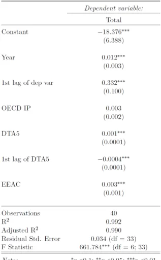
back-casting MAPE shows that the highest performing model for total scrap supply can be expressed via Equation 2 and the coefficients provided in Table 1.
Totalt=c+αt+γ Totalt−1+β1OECDIPt+β2DTA 5t+β3DTA 5t −1+β4EEACt+εt(2)
The ARDL model residuals also do not show significant autocorrelation for the first few terms as shown in the supporting information.
Table 1. Summary of the highest performing ARDL model for total scrap supply 208 209 210 211 212 213 214 215 216 217 218 219 220 221 222 223 224
Assuming the variables in the model are stable in the long run2, the long run effect from
OECDIP, DTA5 and EEAC is β1 1−γ,
β2+β3 1−γ ,
β4
1−γ respectively, and the values are 5.2×10⁻³, 2.5×10⁻⁴, 4.9×10⁻³. Since the values of all three explanatory variables are
around 100, this means that +1% change in OECDIP and EEAC would lead to approximately +0.5% change in copper scrap supply, while +1% in DTA5 would only lead to about +0.025% change. Therefore, we interpret that OECDIP and EEAC are the two main drivers of total copper scrap supply. In market equilibrium models, the equilibrium quantity we observe is influenced by supply shifters and demand shifters simultaneously (Mankiw, 2006). Our model reflects this theory as OECDIP is a supply shifter for the level of industrial production in developed countries, while EEAC reflects the level of manufacturing (and therefore demand) for electrical products, an end use that accounted for more than 20% of copper demand in 2012 (Kelly et al. , 2010).
The regression coefficients for OECDIP and EEAC are positive, i.e. everything else equal, an increase in either independent variable correlates with an increase in scrap supply. This follows our intuition for the behavior of scrap availability as a function of changes in IP index where increased industrial activity is likely to boost both the source of scrap (e.g. increased demolition and manufacturing) as well as processed scrap demand (e.g. from brass mills). A positive relationship between materials supply and industrial activity has also been found for primary metal (Binder et al. , 2006). We also observe that the regression coefficient for the lagged dependent variable is positive and less than one. This means that an increase in scrap supply is likely to be followed by further increase in succeeding years, everything else equal. Conversely, a decrease in scrap volume is more likely succeeded by further decrease than an increase. This may suggest that scrap which is not collected in year t (because of factors such as price and industrial activity) may not necessarily be available in year t+1. In line with this, others have found that old scrap stocks, the stock of copper having reached its end-of-life without being recycled, have a very modest impact on the production of secondary copper (Gomez, Guzman, 2007). At least to some degree this correlation suggests whether or not the metal may be recycled at all. Metal products reaching their end-of-life in a year with falling industrial production may not simply be set aside for recycling in more prosperous years – they may never be recycled (Blomberg and Soderholm, 2009).
Lastly, we note that we found no significant correlation between secondary and primary copper supply even when not correcting for IP and price. While links between primary and secondary metal markets exist, especially in terms of price and volatility (Xiarchos and Fletcher, 2009), our results suggest that the supply of secondary copper is not strongly correlated with the supply of primary copper.
In this first result, we treated different categories of copper scrap supply together. However, since the dataset (and metallurgical reality) of copper scrap is partitioned into high quality scrap (direct melt scrap) and low quality scrap (refined scrap), we also investigate
2 In the ARDL model, the short run effect of an explanatory variable is directly represented by the estimated regression coefficient, while the long run effect is estimated assuming that the variable of interest is stable in time. For example, we assume that scrap supply is stable, therefore
Totalt=Totalt −1=^Total , the long run effect of OECDIP is ∂OECDIP∂ ^Total =
β1 1−γ . 225 226 227 228 229 230 231 232 233 234 235 236 237 238 239 240 241 242 243 244 245 246 247 248 249 250 251 252 253 254 255 256 257 258 259 260 261 262 5 6 7 8
these two scrap populations independently to understand whether the drivers behind them are different.
3.2 Direct Melt Scrap
We now focus on models for which direct melt scrap volumes are the dependent variable. In this case variable grouping and forward stepwise variable selection yields three explanatory variables: United States Industrial Production Index (USIP), HVAC, metalworking, and power transmission machinery Index (IPDG) and EEAC. Time is again forced in the model. The ACF plot of the OLS model exhibits significant autocorrelation, and the highest performing back-casting MAPE ARDL model is summarized in Table 2 (with details in the supporting information).
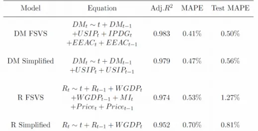
Table 2. Summary of the best ARDL model for direct melt scrap supply, termed DM FSVS (direct melt forward stepwise variable selection)
The long run effects from USIP, IPDG and EEAC are 2.2×10⁻², -3.3×10⁻³, 4.0×10⁻³
respectively. All three indicators are normalized to a scale of 100, so with +1% change in the three variables, direct melt copper scrap supply would change approximately 2.2%, -0.33% and 0.4% respectively. It is clear that among the three variables, USIP is the main driver of scrap supply. Although the USIP index is calculated only for US, its time series is very similar to OECDIP (ρ = 0.99). Therefore, we interpret from the estimated regression 263 264 265 266 267 268 269 270 271 272 273 274 275 276 277 278 279 280 281 282 283
coefficients that direct melt copper scrap supply is driven by level of industrial production activity for developed countries.
The complexity of this model (which we will refer to as DM FSVS – direct melt forward stepwise variable selection) lies on the edge of Harrell’s rule of thumb which requires that a minimum of 10 observations are required per each explanatory variable). Therefore, in order to further reduce the risk of over-fitting, we test (based on our cross-validated back casting MAPE) a simpler ARDL model (DM simplified) where we start with an OLS model that only includes year and USIP (based on the strength of the correlation with USIP described above). This DM simplified model is summarized in Table 3 and does not show significant autocorrelation.
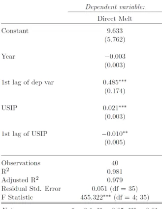
Table 3. Summary of the best performing simplified model for direct melt scrap supply, termed DM simplified
The long run effect from USIP is 0.021, which means that everything else being equal, a +1% change in USIP would lead to approximately +2.1% change in direct melt copper scrap supply. We find that the performance of the DM simplified model developed by choosing the variable with strongest dependence is similar to our more complex model found through forward stepwise variable selection. DM FSVS and DM simplified exhibit similar adjusted r2,
and MAPE values. We summarize this DM model comparison along with the model for refined scrap found in the next section in Table 6 (and section 3.4). The Test MAPE shown in the table is the back-casting MAPE using 1972~2002 data as the training set and 2003~2012 data as the test set.
284 285 286 287 288 289 290 291 292 293 294 295 296 297 298 299 300 301 302 303 304 305 306 307 308
3.3 Refined Scrap
We then use refined scrap volumes as the dependent variable and perform the regression analysis, following the same procedure. After variable grouping and forward stepwise variable selection, three explanatory variables are included in the refined (R FSVS) model: world GDP (WGDP), Mining Index (MI) and real refined copper price, and a year variable is again forced in the model. ACF plot of the OLS model exhibits significant autocorrelation (Figure S2), and the best performing R FSVS ARDL model selected is summarized in Table 4.
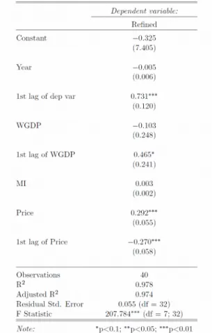
Table 4. Summary of the best performing model for refined scrap supply, termed R FSVS
The long run effects from WGDP, MI and price are 1.35, 0.011 and 0.082 respectively. Since WGDP and price are already log transformed, the estimated regression coefficients can be directly interpreted as supply elasticities (Blomberg and Soderholm, 2009). This means that +1% change in world GDP and copper price would lead to +1.35% change and 0.08% change in refined copper scrap supply, respectively. Given that values of MI are normalized to a scale of 100, +1% change in MI would lead to about +1.1% change in refined copper scrap supply.
Previous work has shown that steel is price inelastic and the demand elasticity is in the range of -0.2 to -0.3 (Malanichev and Vorobyev, 2011). Therefore,based on the estimated price elasticity, we argue that refined copper scrap supply is price inelastic, and its main drivers are world GDP and level of mining activity. MI on the other hand, reflects the 309 310 311 312 313 314 315 316 317 318 319 320 321 322 323 324 325 326 327 328 329 330 331
manufacturing output of the entire mining industry in US, and therefore can be seen as a supply shifter that affects copper supply in a general way.
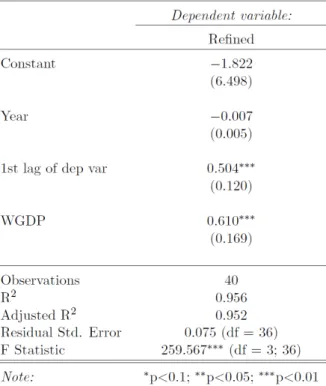
World GDP is an approximation of global income growth rate and reflects demand of products in general. It can, therefore, be considered as a demand shifter in general accordance with economic theory. Since the long run effects from world GDP is the greatest among three variables, we also explore a simpler ARDL model (R simplified) similar to the one we develop for direct melt copper scrap. We start with an OLS model that only includes year and WGDP, and select the best back-casting MAPE ARDL model, which is summarized in Table 5.
Table 5. Summary of the best performing simple model for refined scrap supply, termed R simplified
We find that the complex model slightly outperforms the simple model in terms of adjusted r2
and MAPE, but the simple model has a significantly lower back-casting MAPE shown in Table 6. We compare the performance of each of the FSVS and simplified models for direct melt and refined in the next section.
We have shown that direct melt copper scrap supply is driven mainly by the level of industrial production in developed countries, while refined copper scrap supply is driven mainly by income growth rate and level of mining activities. In addition, the simplified ARDL models for direct melt and refined scrap, which include only one explanatory variable, offer similar or better performance compared to the complex models.
We see limited dependence of copper supply on price. Refined scrap, the lower quality portion of the two, correlates in a limited way with price (and indirectly through GDP), but not with industrial activity. Direct melt scrap, the higher quality portion of the two, correlates with industrial activity, but not with price. The low own-price elasticity of secondary refined copper production of 0.08 is comparable to previous findings from 332 333 334 335 336 337 338 339 340 341 342 343 344 345 346 347 348 349 350 351 352 353 354 355 356 357 358
secondary materials, such as copper (0.25 to 0.29), aluminum (0.18 to 0.32) and paper (0.20-0.30)(Blomberg and Soderholm, 2009, Fisher et al. , 1972, Mansikkasalo, Lundmark, 2014). The relatively low own-price elasticity of recycled material supply is in part due to its dependence on past consumption patterns.
3.4 Model performance comparison
In section 3.1, we did not differentiate high quality copper scrap from low quality scrap, and demonstrated that two main drivers of total scrap supply were OECDIP and EEAC, which reflect levels of industrial production in developed countries and production of electrical products. On the other hand, our independent models for direct melt scrap and refined scrap contained USIP as the most important driver for direct melt scrap and WGDP for refined scrap. Although these are different variables from the ones in the total scrap model, they essentially reflect the same categories of drivers of scrap availability: OECDIP and USIP both reflect how industrial production in developed countries drives supply of copper scrap, while EEAC reflect drivers for copper demand in a specific end-use sector and WGDP for copper demand in general.
Here we compare model performance to synthesize our findings on what drives copper scrap availability. First, Figure 1 plots the FSVS (red lines) and simplified (blue lines) models for direct melt (circles) and refined (triangles) copper along with the actual historic data on copper scrap supply (black lines). The similarity among the lines for each scrap type is clear and Table 6 summarizes the quantitative comparison between the FSVS and simplified models. 359 360 361 362 363 364 365 366 367 368 369 370 371 372 373 374 375 376 377 378 379 380 381 382
Figure 1. Comparison of FSVS (red) and simplified (blue) econometric models for direct melt (circles) and refined (triangles) scrap with actual historic copper scrap supply (black) in
kilotons.
Table 6. Comparison of simplified and FSVS models for direct melt and refined scrap supply
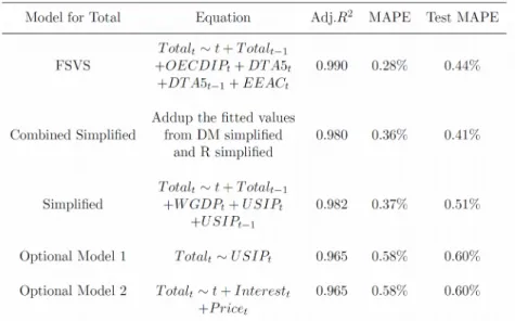
Now that we have independent models for direct melt scrap and refined scrap, we develop two additional models for total copper scrap supply and compare model performance. The first additional model adds up the fitted variables of direct melt scrap and refined scrap from the simple ARDL models (combined simplified). The second model performs an independent regression including the variables used in the two independent simple ARDL models (simplified). In order to demonstrate that the variables included are important, we also add two other models for comparison. The first is a model that only includes lead terms USIP (Optional model 1), and the second includes two less significant variables which are 10 year interest rate (Constant Maturity Rate) and price (Optional model 2). The performance of these four models compared with the total FSVS model developed in section 3.1 is summarized in Table 7. 383 384 385 386 387 388 389 390 391 392 393 394 395 396 397 398 399 400 401 402
Table 7. Comparison of different econometric models for total scrap supply We find that the first three models in Table 7 perform similarly. The FSVS model, our ‘complex’ model for total scrap supply, is the best model in terms of fitting. Combined simplified, the add-up of two simplified ARDL models, is the best in terms of predictive power. All three have improved performance over the other models in Table 7.
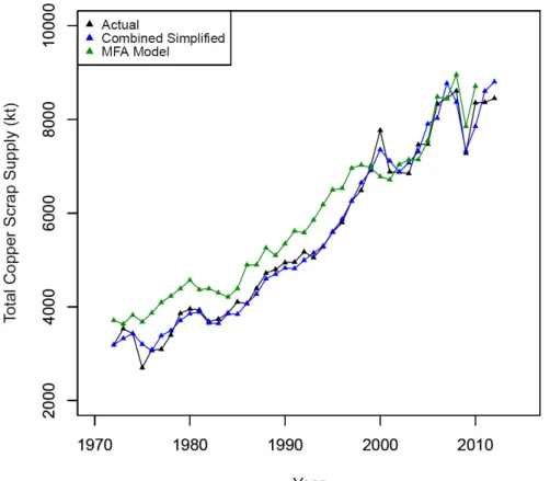
One of our motivations for this econometric study of copper scrap supply was as a complementary approach to material flow analysis (MFA) to quantify copper scrap supply (or potential supply). An example of the differences between these approaches is shown in Figure 2, where we’ve plotted MFA results by Gloser et al. (Gloser, Soulier, 2013), along with the fitted values from the combined simplified model, which we have chosen based on its predictive performance. We see improved performance for the econometric model over the MFA model for certain time periods. In addition, the MAPE of the combined simplified model is 0.36%, while the MAPE of MFA is 1.27%. This observation, in addition to the relatively lower effort and data requirements of econometric modeling make it an attractive route for short term estimation. In addition to the estimates shown in Figure 2, however, the two methods produce an array of useful information and are complementary. For example, while the MFA model yields collection rates of waste types, econometric models may shed light on how efficient incentives can be at improving those rates.
403 404 405 406 407 408 409 410 411 412 413 414 415 416 417 418 419 420 421 422 423
Figure 2. Comparison of econometric “combined simplified” model, MFA results (Gloser, Soulier, 2013) and historic copper scrap supply in kilotons
4. Conclusion
We have adopted and modified an approach to develop a set of econometric models for quantifying secondary copper supply. Our investigation of econometric drivers of scrap availability led to several conclusions that we summarize here. Total scrap is most strongly correlated with variables such as the OECD Industrial Production and production indices of copper-containing products, such as electrical equipment and appliances. We found that an increase in either of these variables corresponds to an increase in scrap supply. Based on incorporation of a lagged term on scrap supply, our model on total scrap supply also suggests that scrap which is not collected in one year may not necessarily be available for collection in subsequent years. Previous work has commented on potential availability of these so called hibernating stocks (Daigo et al. , 2015). This potential for scrap hibernation indicates that incentives should focus on capturing material as soon as scrap is generated or focus on reduction of collection costs.
The models that we developed independently for direct melt (higher quality) and refined scrap demonstrated complementary correlations. Our model of direct melt scrap correlates most strongly with the Industrial Production index for the US, while for refined scrap the dependence is dominated by world GDP and mining activity, with a limited correlation with price. More generally, direct melt scrap availability demonstrates stronger dependence on so-called supply shifting variables, while refined scrap depends more on demand shifting variables. Finally, we have shown that the performance of these econometric models performs as well or better than an MFA-derived model of historic scrap supply, and, 424 425 426 427 428 429 430 431 432 433 434 435 436 437 438 439 440 441 442 443 444 445 446 447 448
therefore, provides an opportunity for a complementary approach to understand flows of recycled material.
The results above suggest that as long as scrap is generated (e.g. through demolition and manufacturing waste) higher quality scrap will be collected and used to produce copper products almost regardless of price. This follows intuition that the collection of lower grade scrap would be more related to the economics of the collectors. The cost of collection (and processing for market) are on the order of the price for this grade of copper meaning that price fluctuations make some forms of collection and processing less attractive, although with limited influence. This is in contrast to the higher value material, where its higher price is effectively always above the threshold that triggers willingness to collect and process. It could be that further processing steps on the lower grade material add a cost to the production of secondary copper cathode that make the industry margins more sensitive to price changes.
The relationship between secondary material supply and explanatory variables has previously been discussed in light of price and quantity based policy strategies (Sigman, 1995). For example, a necessary condition for price-based policies to be effective is some correlation between material supply and price (Blomberg and Soderholm, 2009). By accounting for the quality of the scrap, the present study takes this discussion one step further: the lower the quality of scrap, the higher the potential impact of price.
Now that we have explored potential drivers of scrap availability, we comment briefly on relevant policy instruments that have been used to influence scrap availability (or to drive increased recycling). Generally market-based policy instruments include tax-subsidy combinations with a disposal fee, deposit-refund (combined output tax and recycling subsidy) and tradeable permit schemes. Research has found that these fees should be matched as closely as possible to the cost of waste disposal or the potential for damage (Calcott and Walls, 2005), but these combined approaches have been found to be more effective than only taxing waste or use of virgin materials (Kinnaman, 2016). These policy instruments can be contrasted with end-of-pipe or more general emissions monitoring on primary alternatives, which act more indirectly to increase recycling and are generally more costly (Soderholm, 2011). We therefore hypothesize that any policy instruments based on price should be directed towards the low-end segment of the scrap market where they may have more impact. This analysis has focused on primary copper price, which may not be as effective a proxy for lower grade scrap. In other words, low quality scrap may have a stronger correlation with primary copper price but is still inelastic to secondary copper prices. Materials that demonstrate own-price inelasticity (as we have demonstrated here) should likely be taxed higher than those which exhibit greater price sensitivity (or these policies may have little impact on recycling rates). Alternatively, we hypothesize that measures directed at demand-side behavior may have stronger impact or policies that facilitate willingness to invest in collection and recycling infrastructure, such as forward contracts. Others have proposed tighter coupling or cooperation between primary and secondary producers (Løvik et al. , 2014), so our findings also show this may be a promising strategy, both in terms of cost effectiveness and potential for increasing scrap availability.
5. Acknowledgements 449 450 451 452 453 454 455 456 457 458 459 460 461 462 463 464 465 466 467 468 469 470 471 472 473 474 475 476 477 478 479 480 481 482 483 484 485 486 487 488 489 490 491
The authors would like to acknowledge funding from the National Science Foundation Award #1605050, Environmental Sustainability Program (ENG-CBET) that provided partial support to make this work possible. The authors are grateful for methodological discussions and input from Randolph Kirchain and Richard Roth.
REFERENCES
Achillas C, Aidonis D, Vlachokostas C, Karagiannidis A, Moussiopoulos N, Loulos V. Depth of manual dismantling analysis: A cost-benefit approach. Waste Manage. 2013;33:948-56. Alonso E, Field FR, Kirchain RE. Platinum Availability for Future Automotive
Technologies. Environ Sci Technol. 2012;46:12986-93.
Alonso E, Gregory J, Field F, Kirchain R. Material availability and the supply chain: Risks, effects, and responses. Environ Sci Technol. 2007;41:6649-56.
Angus A, Casado MR, Fitzsimons D. Exploring the usefulness of a simple linear regression model for understanding price movements of selected recycled materials in the UK.
Resources Conservation and Recycling. 2012;60:10-9.
Azadeh A, Neshat N, Mardan E, Saberi M. Optimization of steel demand forecasting with complex and uncertain economic inputs by an integrated neural network-fuzzy mathematical programming approach. Int J Adv Manuf Tech. 2013;65:833-41.
Baffes J, Savescu C. Monetary conditions and metal prices. Appl Econ Lett. 2014;21:447-52. Bertram M, Graedel TE, Rechberger H, Spatari S. The contemporary European copper cycle: waste management subsystem. Ecological Economics. 2002;42:43-57.
Binder CR, Graedel TE, Reck B. Explanatory variables for per capita stocks and flows of copper and zinc - A comparative statistical analysis. J Ind Ecol. 2006;10:111-32.
Blomberg J, Soderholm P. The economics of secondary aluminium supply: An econometric analysis based on European data. Resources Conservation and Recycling. 2009;53:455-63. Calcott P, Walls M. Waste, Recycling, and Design for Environment. Resource and Energy Economics. 2005;27:287-305.
Chen WQ. Recycling Rates of Aluminum in the United States. J Ind Ecol. 2013;17:926-38. Cullen JM, Allwood JM. Mapping the Global Flow of Aluminum: From Liquid Aluminum to End-Use Goods. Environ Sci Technol. 2013;47:3057-64.
Daigo I, Iwata K, Ohkata I, Goto Y. Macroscopic evidence for the hibernating behavior of materials stock. Environ Sci Technol. 2015;49:8691-6.
Elshkaki A, van der Voet E, Timmermans V, Van Holderbeke M. Dynamic stock modelling: A method for the identification and estimation of future waste streams and emissions based on past production and product stock characteristics. Energy. 2005;30:1353-63.
Finnveden G, Ekvall T, Arushanyan Y, Bisaillon M, Henriksson G, Ostling UG, et al. Policy Instruments towards a Sustainable Waste Management. Sustainability-Basel. 2013;5:841-81. Fisher FM, Cootner PH, Bailey MN. Econometric Model of World Copper Industry. Bell J Econ. 1972;3:568-609.
Flores GRFA, Nikolic S, Mackey PJ. ISASMELT (TM) for the Recycling of E-Scrap and Copper in the U.S. Case Study Example of a New Compact Recycling Plant. Jom-Us. 2014;66:823-32.
Gaustad G, Olivetti E, Kirchain R. Design for Recycling. J Ind Ecol. 2010;14:286-308. Gleich B, Achzet B, Mayer H, Rathgeber A. An empirical approach to determine specific weights of driving factors for the price of commodities-A contribution to the measurement of the economic scarcity of minerals and metals. Resour Policy. 2013;38:350-62.
Gloser S, Soulier M, Espinoza LAT. Dynamic Analysis of Global Copper Flows. Global Stocks, Postconsumer Material Flows, Recycling Indicators, and Uncertainty Evaluation. Environ Sci Technol. 2013;47:6564-72.
492 493 494 495 496 497 498 499 500 501 502 503 504 505 506 507 508 509 510 511 512 513 514 515 516 517 518 519 520 521 522 523 524 525 526 527 528 529 530 531 532 533 534 535 536 537 538 539 540
Gomez F, Guzman JI, Tilton JE. Copper recycling and scrap availability. Resour Policy. 2007;32:183-90.
Gsodam P, Lassnig M, Kreuzeder A, Mrotzek M. The Austrian silver cycle: A material flow analysis. Resources Conservation and Recycling. 2014;88:76-84.
Habuer, Nakatani J, Moriguchi Y. Time-series product and substance flow analyses of end-of-life electrical and electronic equipment in China. Waste Manage. 2014;34:489-97. Hamilton JD. Time series analysis: Princeton university press Princeton; 1994.
Harrell F. Regression modeling strategies: with applications to linear models, logistic and ordinal regression, and survival analysis: Springer; 2015.
ICSG. The World Copper Factbook. 2013.
Kelly TD, Matos GR, Buckingham D, DiFrancesco C, Porter K, Berry C, et al. Historical statistics for mineral and material commodities in the United States. US Geological Survey data series. 2010;140.
Kinnaman TC. Understanding the Economics of Waste: Drivers, Policies, and External Costs. International Review of Environmental and Resource Economics. 2016;8:281-320.
Lifset RJ, Eckelman MJ, Harper EM, Hausfather Z, Urbina G. Metal lost and found: Dissipative uses and releases of copper in the United States 1975-2000. Sci Total Environ. 2012;417:138-47.
Liu G, Muller DB. Centennial Evolution of Aluminum In-Use Stocks on Our Aluminized Planet. Environ Sci Technol. 2013;47:4882-8.
Løvik AN, Modaresi R, Müller DB. Long-Term Strategies for Increased Recycling of Automotive Aluminum and Its Alloying Elements. Environ Sci Technol. 2014;48:4257-65. Malanichev A, Vorobyev P. Forecast of global steel prices. Studies on Russian Economic Development. 2011;22:304-11.
Mankiw N. Principles of microeconomics: Cengage Learning; 2006.
Mansikkasalo A, Lundmark R, Soderholm P. Market behavior and policy in the recycled paper industry: A critical survey of price elasticity research. Forest Policy Econ. 2014;38:17-29.
McMillan CA, Moore MR, Keoleian GA, Bulkley JW. Quantifying US aluminum in-use stocks and their relationship with economic output. Ecological Economics. 2010;69:2606-13. Muller E, Hilty LM, Widmer R, Schluep M, Faulstich M. Modeling Metal Stocks and Flows: A Review of Dynamic Material Flow Analysis Methods. Environ Sci Technol.
2014;48:2102-13.
Northey S, Mohr S, Mudd GM, Weng Z, Giurco D. Modelling future copper ore grade decline based on a detailed assessment of copper resources and mining. Resources Conservation and Recycling. 2014;83:190-201.
Olivetti EA, Gaustad GG, Field FR, Kirchain RE. Increasing Secondary and Renewable Material Use: A Chance Constrained Modeling Approach To Manage Feedstock Quality Variation. Environ Sci Technol. 2011;45:4118-26.
Rankin WJ. Minerals, Metals and Sustainability Meeting Future Material Needs An
introduction to sustainability. Minerals, Metals and Sustainability: Meeting Future Material Needs. 2011:41-61.
Reck BK, Graedel TE. Challenges in Metal Recycling. Science. 2012;337:690-5.
Rubin RS, de Castro MAS, Brandao D, Schalch V, Ometto AR. Utilization of Life Cycle Assessment methodology to compare two strategies for recovery of copper from printed circuit board scrap. J Clean Prod. 2014;64:297-305.
Ruth M. Thermodynamic constraints on optimal depletion of copper and aluminum in the United States: A dynamic model of substitution and technical change. Ecological Economics. 1995;15:197-213. 541 542 543 544 545 546 547 548 549 550 551 552 553 554 555 556 557 558 559 560 561 562 563 564 565 566 567 568 569 570 571 572 573 574 575 576 577 578 579 580 581 582 583 584 585 586 587 588 589
Sigman HA. A Comparison of Public Policies for Lead Recycling. Rand J Econ. 1995;26:452-78.
Slade ME. An Econometric-Model of the United-States Secondary Copper-Industry - Recycling Versus Disposal. Journal of Environmental Economics and Management. 1980;7:123-41.
Slade ME. Trends in natural-resource commodity prices: An analysis of the time domain. Journal of Environmental Economics and Management. 1982;9:122-37.
Soderholm P. Taxing virgin natural resources: Lessons from aggregates taxation in Europe. Resources Conservation and Recycling. 2011;55:911-22.
Soderholm P, Tilton JE. Material efficiency: An economic perspective. Resources Conservation and Recycling. 2012;61:75-82.
Solow RM. Economics of Resources or Resources of Economics. Am Econ Rev. 1974;64:1-14.
Wagenhals G. The World Copper Market - Structure and Econometric-Model. Lect Notes Econ Math. 1984;233:R3-+.
Wang P, Jiang ZY, Geng XY, Hao SY, Zhang XX. Quantification of Chinese steel cycle flow: Historical status and future options. Resources Conservation and Recycling. 2014;87:191-9.
Wubbeke J, Heroth T. Challenges and political solutions for steel recycling in China. Resources Conservation and Recycling. 2014;87:1-7.
Xiarchos IM, Fletcher JJ. Price and volatility transmission between primary and scrap metal markets. Resources Conservation and Recycling. 2009;53:664-73.
590 591 592 593 594 595 596 597 598 599 600 601 602 603 604 605 606 607 608 609 610 611 612