Dropped object detection in crowded scenes

Dropped Object Detection in Crowded Scenes

by

Deepti Bhatnagar

A

B.Tech., Indian Institute of Technology Delhi (2007) Li

_LIt

HUSETTS INSTnfUTE

TECHNOLOGY

IG

0

7

2009

3RARIES

Submitted to the Department of Electrical Engineering and Computer

Science

in partial fulfillment of the requirements for the degree of

Master of Science

in Electrical Engineering and Computer Science

at the

MASSACHUSETTS INSTITUTE OF TECHNOLOGY

June 2009

@ Massachusetts Institute of Technology 2009. All rights reserved.

ARCHIVES

A uthor ...

Department of Electrical Erineering and Computer Science

May 22, 2009

Certified by...

Prof. W. Eric L. Grimson

Bernard Gordon Professor of Medical Engineering

Thesis Supervisor

Accepted by ...

/

Terry Orlando

TeChairman,

rry Orlando

Department

Committee

on

G

Chairman, Department Committee on Graduate Students

Dropped Object Detection in Crowded Scenes

by

Deepti Bhatnagar

B.Tech., Indian Institute of Technology Delhi (2007)

Submitted to the Department of Electrical Engineering and Computer Science on May 22, 2009, in partial fulfillment of the

requirements for the degree of Master of Science

in Electrical Engineering and Computer Science

Abstract

In the last decade, the topic of automated surveillance has become very important in the computer vision community. Especially important is the protection of critical transportation places and infrastructure like airport and railway stations. As a step in that direction, we consider the problem of detecting abandoned objects in a crowded scene. Assuming that the scene is being captured through a mid-field static camera, our approach consists of segmenting the foreground from the background and then using a change analyzer to detect any objects which meet certain criteria.

In this thesis, we describe a background model and a method of bootstrapping that model in the presence of foreign objects in the foreground. We then use a Markov Random Field formulation to segment the foreground in image frames sampled peri-odically from the video camera. We use a change analyzer to detect foreground blobs that remain static through the scene and based on certain rules decide if the blob could be a potentially abandoned object.

Thesis Supervisor: Prof. W. Eric L. Grimson

Acknowledgments

I would like to thank my advisor Prof. Eric Grimson for his guidance, direction and encouragement. I am grateful to him for his patience, especially during my initial years at grad school. It is an honor and great pleasure to be advised by him.

This work greatly benefited from the ideas and discussions with all the people in CSAIL and APP. I thank them all for the many insightful discussions.

Words cannot express my feelings towards my parents, Mrs. Preeti Bhatnagar and Mr. Pradeep Bhatnagar, for their love, encouragement and sacrifice. This thesis is dedicated to them. I express a feeling of bliss for having a loving sister like Ms. Shikha Bhatnagar. I would also like to thank all my friends and family for their unconditional love, support and encouragement.

Contents

1 Introduction

1.1 Activity Analysis ...

1.2 Abandoned Object Detection in 1.2.1 Motivation ...

1.2.2 Other Applications . . . 1.2.3 Discussion ...

1.3 Problem Statement ...

1.4 Outline of our Approach . . . . 1.4.1 Our Contributions . . . 1.5 Organization of the Thesis . . .

. . . . . . . . . . Crowded Scenes . . . . . . . . . . . . . . . . . . . . . . . . . . . . . . . . . . . . . . . . . . . . . . . . . . . . . . . . . . . . . . . . . . . . . . .

2 Abandoned Object Detection: A Review

2.1 2.2 2.3 2.4

Related Work: Activity Monitoring in Unconstrained Settings Related Work: Object Tracking . ...

Related Work: Abandoned Object Detection ... Where This Thesis Fits In . ...

3 Foreground Extraction Using Energy Minimization 3.1 Background Model . ...

3.2 Model Description ... 3.2.1 Model Parameters ... 3.2.2 Parameter Computation . ...

3.2.3 Bootstrapping the Model ... 7 11 12 13 13 14 14 16 16 20 22

3.3 Foreground Extraction with Graph Cuts . ... . 36

4 Change Analysis and Abandoned Object Detection 43 4.1 Potential Static Blob Identification . ... 44

4.2 Region Classification for Abandoned Object Detection . ... 46

4.2.1 Deciding Whether the Entity is Moving or Static ... . 47

4.2.2 Deciding Whether the Entity is Living or Non-Living .... . 49

4.2.3 Deciding Whether the Object could be Abandoned ... 52

4.2.4 Exam ples ... .. .. . . . . .. .. ... ... .... 53

5 Assessment and Evaluation 55 5.1 D atasets . . . .. .. . 55

5.2 Background Model ... ... 56

5.3 Foreground Segmentation ... 58

5.4 Abandoned Object Detection ... 75

List of Figures

1-1 Background image for sample dataset S7 from PETS-2007 ... 17

1-2 Frame from sample dataset S7 ... 18

1-3 Extracted foreground using our technique . ... 19

1-4 Abandoned object detection in the sample frame . ... 20

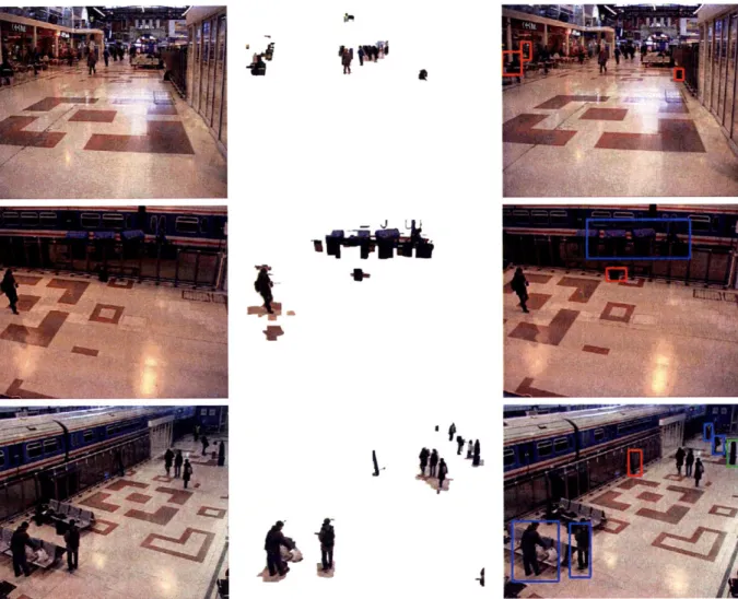
1-5 Results for other sample datasets from PETS-2006 . ... 21

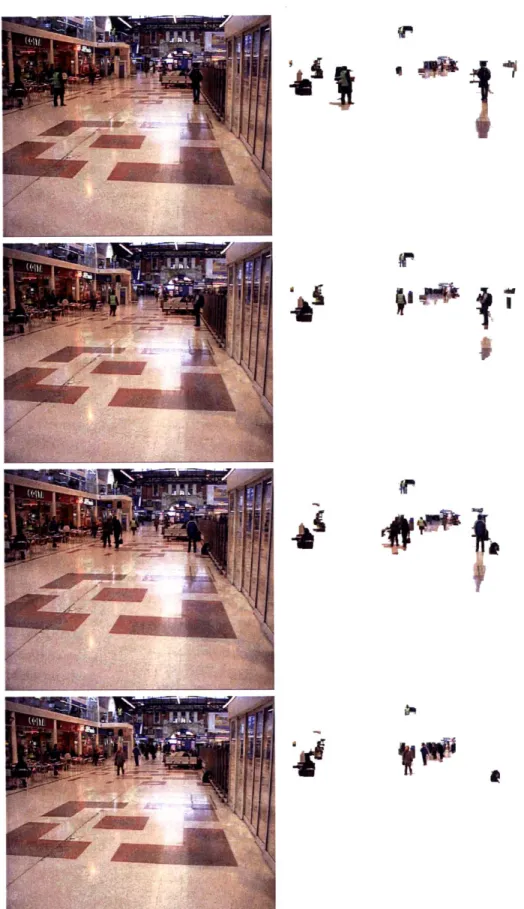
3-1 Extracted foregrounds for dataset S1 from PETS-2006 . ... 38

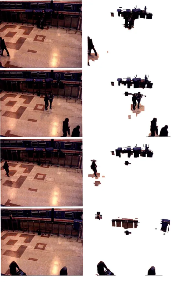
3-2 Extracted foregrounds for dataset S2 from PETS-2006 . ... 39

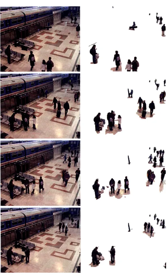
3-3 Extracted foregrounds for dataset S5 from PETS-2006 . ... 40

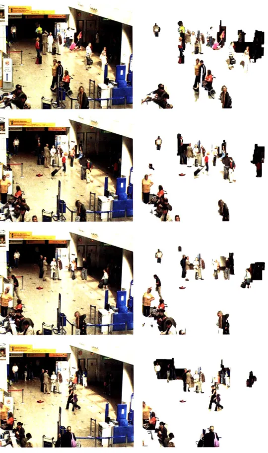
3-4 Extracted foregrounds for dataset S7 from PETS-2007 . ... 41

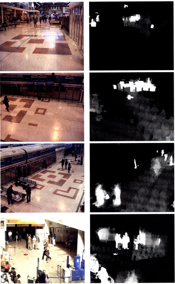
4-1 Moving average image, MA, in sample datasets . ... 45

4-2 Moving average image, MF, in sample datasets . ... 48

4-3 Examples showing observable jitter in living entities ... 50

4-4 Examples showing no observable jitter in non-living entities ... 50

4-5 Earliest frame where the object appears compared with the current frame ... ... 52

4-6 Abandoned object detection in sample datasets . ... 54

5-1 Background Image for all four datasets . ... 57

5-2 Foreground results for dataset S1 from PETS-2006: Example 1 . . . . 59

5-3 Foreground results for dataset S1 from PETS-2006: Example 2 . . . . 60

5-4 Foreground results for dataset S1 from PETS-2006: Example 3 . . .. 61

5-6 5-7 5-8 5-9 5-10 5-11 5-12 5-13 5-14 5-15 5-16 5-17 5-18 5-19 5-20 5-21

Foreground results for dataset S2 from PETS-2006: Foreground results for dataset S2 from PETS-2006: Foreground results for dataset S2 from PETS-2006: Foreground results for dataset S2 from PETS-2006: Foreground results for dataset S5 from PETS-2006: Foreground results for dataset S5 from PETS-2006: Foreground results for dataset S5 from PETS-2006: Foreground results for dataset S5 from PETS-2006: Foreground results for dataset S7 from PETS-2007: Foreground results for dataset S7 from PETS-2007: Foreground results for dataset S7 from PETS-2007: Foreground results for dataset S7 from PETS-2007: Sample results for dataset S1 from PETS-2006 Sample results for dataset S2 from PETS-2006 Sample results for dataset S5 from PETS-2006 . Sample results for dataset S7 from PETS-2007 .

Example 1 . Example 2 . Example 3 . Example 4 . Example 1 . Example 2 . Example 3 . Example 4 . Example 1. Example 2 . Example 3 . Example 4 .

Chapter 1

Introduction

Computer Vision is an active area of research, with the goal of developing techniques that can enable artificial systems to better understand the world in an automated way.

To achieve this goal, we need to extract meaningful information and patterns from the images and video clips given to us. The image data itself can take many forms, such as views from multiple cameras or multi-dimensional or multi-modal data. Moreover, we should be able to leverage that information to aid us in creation of systems that control processes, detect events, organize information, and model interactions.

Some of the interesting problems in which the computer vision community has been traditionally interested include object recognition, scene reconstruction, motion tracking, image restoration, and activity analysis in videos.

Activity analysis is the term given to the broad set of techniques that are used to analyze the contents of a video clip to recover activities of interest. An activity consists of an agent performing a series of actions in a specific temporal order.

The area of activity analysis is extremely important in terms of its scope and potential impact. If we can solve the problem, it would have significant implications on the way we organize and search for information. It can significantly benefit us in ways ranging from social science research (like crowd behavior analysis) to auto-mated monitoring in surveillance videos. We have such large amounts of information

captured in videos that could prove to be extremely helpful to mankind if we can interpret it and represent it in ways that are useful.

In this chapter we will motivate the problem of activity analysis and define it more clearly. We will illustrate the challenges that lie along the way and provide some preliminary examples.

1.1

Activity Analysis

Even though the potential applications of activity analysis are growing very fast, the concept of activity still remains mostly elusive for artificial systems. There are several reasons as to why that could be the case.

First is the problem of definition. Many activities are very subjectively defined. For example, consider a surveillance setting that does theft detection or tries to classify anti-social activities. There is no clear cut definition of what constitutes a theft, or an anti-social activity. The classification is difficult even for humans, let alone artificial systems.

Second is the problem of representation. The concept of an activity comes nat-urally to humans. But for a computer, it is very hard to represent an activity in any meaningful format. To be able to abstract an activity, a computer needs to be fully aware of the agents, the actions they are performing and in some cases, their intentions as well. It is difficult to represent this information in terms of rules or observable variables. This is because an occurrence in itself does not mean anything, it has to be taken into account with all the contextual information. Even then, the notion of activity is highly subjective and cannot be easily quantified.

Third is the problem of implementation. Even if we define an activity precisely and devise an appropriate representation, it is still very difficult to detect its occurrence in every case.

There are several reasons as to why looking for instances of an activities in a video clip is hard. To understand the actors in a clip, we need to analyze the image frames at every instant of time and discern all the different objects that are present

in it. Furthermore, we need to recover the actions by analyzing how the objects are changing over the course of time and how they are interacting with each other.

Extracting the objects present in a scene, technically called object segmentation, is a computationally hard task and remains an unsolved problem. Although, there have been many advances in the last few years, a universal solution continues to elude us. And unless we make significant progress in object segmentation and classification, developing a generic activity analyzer seems improbable.

Having concluded that a generic activity analyzer is unlikely in the near-future, the question that faces us is whether we can develop techniques that can let us analyze specific types of activities in a predefined setting without fully solving the object segmentation and classification problem.

The prerequisite for such a system would be a technique that does not deal with objects as the basic building block but rather operates at a much lower pixel level and considers an entity as a set of pixels. The problem of abandoned object detection with which we are dealing helps to illustrate this approach to activity analysis.

1.2

Abandoned Object Detection in Crowded Scenes

1.2.1

Motivation

In the last decade the topic of automated surveillance has become very important in the field of activity analysis. Within the realm of automated surveillance, much emphasis is being laid on the protection of transportation sites and infrastructure like airport and railway stations. These places are the lifeline of the economy and thus particularly prone to attacks. It is difficult to monitor these places manually because of two main reasons. First, it would be very labor intensive and thus a very expensive proposition. Second, it is not humanly possible to continuously monitor a scene for an extended period of time, as it requires a lot of concentration. Therefore, as a step in that direction, we need an automated system that can assist the security personnel in their surveillance tasks. Since a common threat to any infrastructure

establishment is through a bomb placed in an abandoned bag, we look at the problem of detecting potentially abandoned objects in the scene.

1.2.2

Other Applications

Even though the problem at which we are looking is very specific in nature, the techniques are fairly general and can be reused in completely different domains to solve other interesting problems.

Examples of areas where these techniques can be employed include retail settings, social science research and human-computer interaction. In retail, it could be rev-olutionary if the activity of the consumers could be analyzed to better understand consumer behavior and improve product placement in the stores. It can also be used to manage queues more efficiently. Similarly, for social science research, activity analysis could yield a significant amount of information on how species tend to behave under different set of circumstances. For example, it can be used to understand such diverse topics as human behavior in crowds, or the behavior of monkeys or bees under differ-ent control conditions. Also, activity analysis could be utilized in human-computer interaction to better understand how humans interact with computer systems and how they could be improved through the use of gesture-based interfaces that rely on certain types of hand-gestures for real-time interaction.

1.2.3

Discussion

There are several ways to interpret the problem of abandoned object detection in crowded scenes. There is still no consensus in the literature on what constitutes an abandoned object. Every major work on this problem has made a different set of assumptions and worked from there.

The set of assumptions that we make are as follows:

* We define an abandoned object as a non-living static entity that is part of the foreground and has been present in the scene for an amount of time greater than a predetermined threshold.

* A foreground object is defined as an entity that is not a part of the background model. It could result from a new object entering the scene or a sudden change in the background.

* There are no vehicles present in the scene. This assumption is realistic for the environments in which we are interested (like airports, train stations etc.).

* The background changes constantly over time.

* The video will be a mid-field domain. The domain of an imaging system is classified based on the resolution at which the objects and its sub-parts are imaged. In a near-field domain, the objects are high resolution and the object sub-parts are clearly visible. In a far-field domain, the object is not clearly visible and no sub-parts are visible. Mid-field lies between the two, the objects as a whole are clearly visible but some of the sub-parts may be just barely visible.

As a preliminary discussion, an obvious approach to solve this problem would be to segment the objects present in every frame and track them over the course of the video clip. Then based on some set of predefined rules, we can classify an object as abandoned and raise a red flag. There are several flaws with this approach. First and foremost, object segmentation is still a hard unsolved problem. Especially in video clips, which tend to have predominantly low resolution images, it is harder still. Adding to the problem is the fact that we expect the scenes to be densely crowded. Second, even though tracking in uncluttered scenes is comparatively reliable, it may simply not be worth the computational effort when we are trying to detect abandoned objects. Therefore, we need a new perspective on the problem and an entirely different approach to solve it. Moreover, we would like to steer clear of hard problems like object segmentation and recognition as far as possible.

1.3

Problem Statement

Given a video sequence captured by a static uncalibrated camera in a mid-field setting, our objective is:

* To develop a reliable system that detects abandoned objects in a crowded scene. As discussed earlier, we define an abandoned object as an entity which is ab-solutely static in the scene for more than a time period T and the perceived owner of the object is not present within a radius of r.

* To propose a systematic method for segmenting the foreground and background in the scene based on a comprehensive background model.

* To make the background model adaptive, so the system adapts to changes which are persistent and does not have to be restarted periodically.

* To create a system which penalizes false negatives more than false positives. * To use techniques which are robust in the presence of dense crowds, like at

airports, train stations, retail stores etc.

1.4

Outline of our Approach

We use a pixel based approach to solve the problem. Our solution is based on a foreground segmentation and statistical analysis technique. We use a statistical back-ground model based on the variation in brightness distortion and chromaticity dis-tortion of every pixel. We model the foreground segmentation problem as a labeling problem and then use a Markov Random Field setup to tackle it.

The segmented foreground is fed to a change analyzer that tries to detect sets of pixel in the image which are consistently being labeled as foreground and to ascertain if that set has been static for some predetermined amount of time (- T).

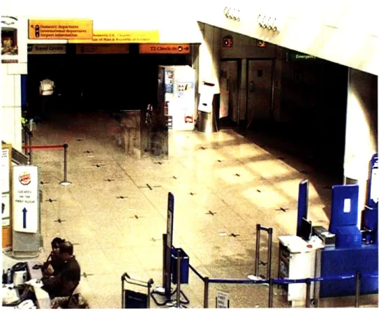
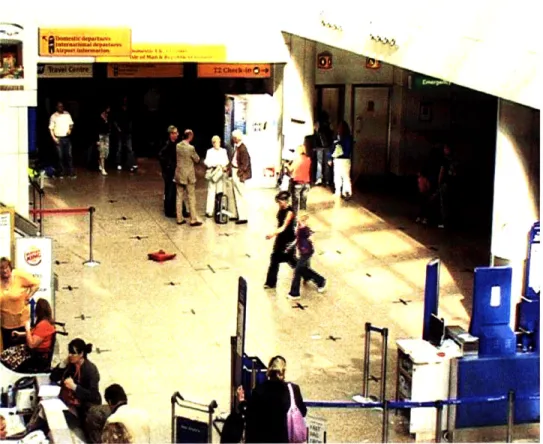
As an example, consider the background scene image shown in Fig. 1-1. For a sample frame shown in Fig. 1-2, we obtain a segmented foreground shown in Fig.

Figure 1-1: Background image for sample dataset S7 from PETS-2007

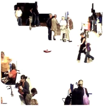
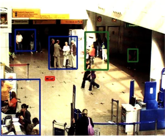
1-3. Feeding it to the change analyzer we obtain the classification shown in Fig. 1-4 where the red box indicates a potentially abandoned object, a blue box indicates a person or a group of people standing in the scene, and a green box indicates people moving through the scene. Fig. 1-5 depicts more such examples for different data sets.

We update our background model at every time step to constantly adapt it to the changing background conditions, at the same time making sure that any abandoned objects are not immediately incorporated into the background.

We try to do this without any priors over the position, orientation, scale or size of the dropped object, in order to make our approach as generic as possible. To classify the entities as living and non-living, we use a Support Vector Machine (SVM). We determine how much an entity has deviated from its position over a certain time period and use that information for classification. According to our analysis, living entities tend to deviate slightly over a period of time. This is because it is difficult for them

Ip-Figure 1-2: Frame from sample dataset S7

to stand absolutely still and even while standing at a place, they show some motion on the fringes of the silhouette. This motion can be captured by cameras in mid-field views. Therefore, we compute the difference of two frames over a predetermined time period and its Discrete Cosine Transform (DCT) over the region of interest. DCT for living entities will have higher coefficients than the non-living ones.

Our approach is based on the principle of minimal evaluation, which says that we should compute a result only if it is required. We will illustrate the use of this principle with the help of two examples. First, when we look for static objects in a scene, we don't track the objects or store their trajectory. This is because all that information is unnecessary if all we are trying to do is single out static objects.

Second, when we classify entities as living or non-living, we do not attempt to determine their exact identity. We are interested in whether the object is living, like a human or a pet, or if the object is non-living like a suitcase or a stroller. We are not interested in object recognition as long as we can make the distinction between

Figure 1-3: Extracted foreground using our technique

living and non-living entities.

The reason we use the principle of minimal evaluation is to prevent the errors in these standard algorithms from accumulating. Computer vision is full of hard problems like segmentation, tracking and object recognition which are not completely solved yet. If we use the object segmentation, classification and tracking approach to

abandoned object detection, the error rate in each of those stages will accumulate. Therefore, it is best in general to avoid a technique that involves solving too many hard problems. It is much more useful to build specific components which are more reliable to the problem at hand.

Having said that, abandoned object detection is not an easy problem and remains particularly challenging for crowded scenes. In dense environments, the objects are usually too close together and there is a lot of occlusion. For that reason, it is difficult to segment the objects or to be able to classify them. Also, it is difficult to track the objects reliably as they move through the scene.

Figure 1-4: Abandoned object detection in the sample frame

1.4.1

Our Contributions

We make four main contributions to the problem of abandoned object detection in crowded scenes.

* A novel approach to initializing and updating the background model in the presence of foreground objects.

* A modified energy minimization formulation of the problem of foreground seg-mentation.

* An efficient pixel based approach to identify whether a foreground blob belongs to an abandoned object.

* A system that maintains minimal state information. We do not need to store large amounts of data in the form of trajectories. This makes the system more scalable by reducing the storage requirements significantly.

-

-J

1.5

Organization of the Thesis

The thesis is organized as follows. Chapter 2 gives an overview of the previous work related to the problem. The scene background model and foreground segmentation technique which forms the basis of our system is described in Chapter 3. Chapter 4 presents our approach for detecting abandoned objects in the scene. Experimental results and analysis are presented in Chapter 5. Chapter 6 summarizes the contribu-tions of our work.

Chapter 2

Abandoned Object Detection: A

Review

This chapter presents an overview of the past work that forms the basis for most of the research on the topic of abandoned object detection in crowded scenes. It also presents various approaches that have been adopted by researchers in the past as an attempt to solve the problem.

Abandoned object detection belongs broadly to the area of activity monitoring in unconstrained settings. In the recent years, significant amounts of work has been done in the field of activity monitoring. Some of that work has been more specific in nature and dealt with a particular subproblem, while others have been more generic.

In this chapter, we will first look at some of the past work in the broad category of activity monitoring. We will then review the topic of object tracking, which forms the basis for most research in this area. Finally, we will look at some of the work on the specific topic of abandoned object detection in crowded scenes.

2.1

Related Work: Activity Monitoring in

Uncon-strained Settings

Most of the work in the field of activity monitoring involves automated flagging of unusual activity in videos. It either entails flagging of individual scenes in a clip or flagging of the entire clip as unusual. Most of that work involves learning from classified examples. Many approaches have been adopted for dealing with the task.

The first category of papers does not involve any tracking of individual objects but rather deals with the entire clip as one entity, which is marked as usual or unusual in entirety [34, 33, 32]. They use motion feature vectors to characterize a clip. Some of these techniques use clustering algorithms to divide the clips into clusters and treat the outliers as unusual. They form an interesting approach but are quite restrictive

for use in surveillance settings because of their inability to account for individual actions.

The second and most common category of papers involves tracking of individual objects in the video and then using statistical analysis to detect anything unusual. They segment the foreground into distinct objects and track each of those objects over time to extract their trajectories. Then using a suitable clustering algorithm, they cluster the trajectories into different clusters. For any new trajectory, they flag it as unusual if it doesn't belong to any of the clusters. Some of these papers also use appearance information to classify the objects into classes like humans, vehicles etc.

To cluster the trajectories, a metric is required to determine the inter-trajectory distance.Various metrics have been proposed in the literature including Euclidean distance [8], Hausdorff distance [16, 31] and hidden markov model based distances [23]. Various clustering techniques have also been proposed including spectral clustering [19], clustering using graph cuts [27] and agglomerative and divisive clustering [2, 18]. Although, trajectory clustering is a very common and well studied approach, there are three main problems that we would like to point out. First, despite all the re-cent advances in the area of object tracking, it remains unreliable in densely crowded scenes. Second, the trajectory of an object is an insufficient indicator of what

consti-tutes unusual in a surveillance setting. An activity could be unusual from a security perspective without having an unusual track and thus, a trajectory does not capture all information about the underlying object. Third, clustering remains ineffective and difficult if we do not know the number of clusters a priori. There are some cluster-ing techniques that do not demand to know the number of clusters; however, these non-parametric techniques are computationally very expensive.

The third category of papers involve a probabilistic approach to activity moni-toring. [20] uses Bayesian framework to determine isolated tracks in a video. [21] uses Coupled Hidden Markov Models to model interactions between two objects. There has also been a rise of non-parametric Bayesian approaches like Dirichlet pro-cess models in recent years. They use a framework like time dependent Dirichlet processes to model the time series data. For example, [7] uses Dirichlet process to solve the problem of data association for multi-target tracking in the presence of an unknown number of targets.

2.2

Related Work: Object Tracking

Since object tracking forms the basis of most research in the area of activity moni-toring, it is useful to understand the evolution of tracking.

In the 1990's, some key advances were made by researchers like Stauffer and Grimson [28] and Haritoaglu [12] in the area of far-field tracking. Since then, a fair amount of work has been done to improve reliability of tracking algorithms in challenging conditions, with lighting changes and dynamic backgrounds

Most tracking methods are based on the technique of background subtraction. They formulate a background model and then compare it with the current frame to find regions of dissimilarity. Then based on some criteria they extract foreground blobs from the scene and then cluster or segment the blobs to form distinct objects

[22, 26, 29, 30].

In sparse settings, these techniques work quite well to detect the objects present along with their associated tracks, but they are not as useful in densely crowded

scenes. Tracking in the presence of dense crowds still remains unreliable.

2.3

Related Work: Abandoned Object Detection

Abandoned object detection is a fairly recent problem in the domain of activity mon-itoring. This is because surveillance became an important topic after the increase of terrorism in different parts of the world and visual surveillance became one of the most active research topics in computer vision.

Increasing concern about security has caused tremendous growth in the number of security cameras present at every important location like airport or railway stations. With so many security cameras doing surveillance at each place, it is extremely labor intensive to have individuals monitor them, which might be an expensive proposi-tion. Besides of this, individuals might get tired or distracted easily and might miss something which is dangerous yet inconspicuous. Hence, it is very useful to have automated systems that can assist the security personnel in their surveillance tasks.

There are three different ways that we can classify the existing research on this topic.

* First is the distinction based on how the scene is being monitored using cameras i.e. single vs. multiple camera setting. In a single camera setting, there is only one camera that monitors a given location, while in a multiple-camera setting there could be multiple cameras monitoring the same location. In case there is more than one camera, the technique can be classified based on whether the multiple cameras are calibrated or not.

* The second distinction is based on the level of granularity of the basic constituents-pixel level approach vs. object level approach. A constituents-pixel level approach does some computation for every pixel and then aggregates the results, while the object level approach detects the objects present in the scene and then does some computation for them.

aban-doned objects. In general, all algorithms for abanaban-doned object detection can be grouped into three categories. First is the set of algorithms based on motion detection- this approach consists of estimating motion for all foreground pix-els/objects present in a scene and then determining the abandoned ones based on certain rules. Second is the set of algorithms based on object segmentation and classification- the scene is segmented into objects which are classified into preexisting classes (like people, luggage) and then they are observed over time to identify the static ones. The third set of techniques involves tracking based analytics- the foreground pixels/objects are tracked over time and their tracks analyzed to detect abandoned objects.

We will now discuss some specific papers that attempt to detect abandoned lug-gage in a crowded setting. [5] deals with a multi-camera setup which detects moving objects using background subtraction. All the information is merged in the ground plane of the public space floor and a heuristic is used to track objects. It detects static luggage and an alarm is triggered when the associated person moves too far. [15] again deals with a multi-camera setup which uses a tracking algorithm based on unscented Kalman filter. It employs a blob object detection system which identifies static objects. It combines the information using homographic transformations and uses a height estimator to distinguish between humans and luggage. [17] tracks ob-jects present in the scene using a trans-dimensional MCMC tracker and analyzes the output in a detection process to identify the static ones. [6] uses a tracking module which tracks blobs and humans using speed, direction and distance between objects. It; uses a Bayesian inference technique to classify abandoned luggage. [11] uses a background subtraction based tracker. It looks for pixel regions in the scene which constantly deviate from the background and flags them as potential abandoned ob-jects. [4] uses a multi-camera object tracking framework. It does object detection using adaptive foreground segmentation based on Gaussian mixtures tracking. It performs centrally in the ground plane, by homographic transformation of the single camera detection results. It does fusion analysis of the object's trajectories, detects stationary objects and splits and merges in the trajectories. [9] does foreground

ex-traction using Markov random fields. It uses a blob tracker as an attention mechanism for finding tracks of interest, extends them temporally using the meanshift algorithm. It; uses weak human and luggage models, based primarily on characteristics like size. [24] has a pixel-based solution that employs dual foregrounds. It models background as multi-layer, multi-variate Gaussian distribution which is adapted using bayesian update mechanism. It fuses multiple cameras on ground plane.

2.4

Where This Thesis Fits In

The approach that we are adopting can broadly be classified as a single camera, pixel level approach. But the algorithm we use to identify abandoned objects is based on analyzing how each pixel changes over time.

Like most other approaches, we build a background model and perform foreground separation for every video frame. But since optical flow computation, object segmen-tation and tracking are unreliable in densely crowded scenes, we adopt a pixel-based solution.

We determine a cohesive set of pixels which are consistently being classified as foreground and analyze how it has been changing over time to determine if the pixels could belong to a potentially dropped object. The advantage of our approach is that it works well under fairly crowded scenarios.

Chapter 3

Foreground Extraction Using

Energy Minimization

This chapter presents the processing steps that are required to extract the foreground from the background in each frame of the video clip. The chapter is divided into two main parts. The first part describes the different components of the background model and the algorithm to initialize them, while the second part describes the algorithm to extract the foreground from the background using an energy minimization technique. We also describe how the results from the foreground extraction can be used to update the background model.

3.1

Background Model

There has been a significant amount of work on background models in computer vision. Most models for background that have been proposed in the literature answer two broad questions. The first question is whether the background model is considered static or dynamic, and accordingly, is it allowed to change over time. The second deals with whether the background is assumed to be a single image which is unknown and has to be estimated using some technique, or is it assumed to be a statistical distribution over an image.

background is assumed to have a unique correct value which has to estimated using some technique like maximum likelihood or energy minimization. Whereas in cases where the background is assumed to have a statistical distribution over an image, every pixel has its own distribution which has to be estimated using some statistical

measures.

Before we delve into our background model, we would like to outline two charac-teristics of the scenes with which we are dealing, so as give more insight into how we answer those questions. First, the image frames that we use to construct our back-ground model are extracted from videos and as a result, their resolution is not very high. Second, the application that we are targeting, i.e. abandoned object detection in crowded scenes, may run for an extended period of time. Over such a long period, there may be significant changes in the lighting conditions and the spatial arrange-ment of objects which are present in the scene. Therefore, we must ensure that these changes are eventually incorporated in the model.

Based on the above characteristics, we have concluded that the background model in our case should be adaptive. Similarly, a statistical model is more suited to our application, as it is more robust in the presence of noise and captures more information about how each pixel might be distributed.

3.2

Model Description

We model our background as a statistical model proposed by Horprasert et al. in [13] and used by Ahn et al. to extract foreground in [1]. It is based on a color model that separates the brightness component of a pixel from its chromaticity component.

The reason we chose this model is because it captures the property of human vision called color constancy, which says that humans tend to assign a constant color to an object even under changing illumination over time or space [14]. Therefore, a color model that separates the brightness from chromaticity component is closer to the model of human vision. Also, to be able to distinguish the foreground from the background pixels we need to differentiate the color of the pixel in the current image

from its expected color in the background. We do this by measuring the brightness and chromatisity distortion for all pixels.

According to the model, the ith pixel in the scene image can be modeled as a 4-tuple < E, si, ai, bi >, where Ei is the expected RGB color value, si is the standard deviation of color value, ai is the variation of the brightness distortion, and bi is the variation of the chromaticity distortion of the ith pixel. The exact mathematical formulation will be described later.

Assuming the brightness distortion and the chromaticity distortion to be normally distributed, we can estimate the likelihood of a pixel belonging to the background using the standard normal distribution.

3.2.1

Model Parameters

More formally, background model estimation consists of estimating the following pa-rameters for each pixel.

* Let E = [pR(i), [G(i), PB(i)] be defined as the ith pixel's expected RGB color

value in the background scene image, where pR(i), PG(i) and sB(i) E [0, 255]. * Let ai = [aR(i), UG(i), B(i)] be defined as the ith pixel's standard deviation in

the RGB color, where aR(i), UG(i) and aB(i) are the standard deviation of the

ith pixel's red, green, blue values measured over a series of M observations. * The brightness distortion (a) is a scalar value that brings the observed color,

Ii, close to the expected chromaticity line, E. In other words, it is the a that

minimizes 0 where

¢(ai) = (Ii - aEi)2 _(3.1)

* Let ai represent the variation of the it_{h pixel's brightness distortion, ai, as}

measured in equation 3.1.

* The chromaticity distortion is defined as the orthogonal distance between the observed color, Ii, and the expected chromaticity line, E. The chromaticity

distortion is given by

CDI = III - aiE | (3.2)

* Let bi represent the variation of the ith pixel's chromaticity distortion, CDi, as measured in equation 3.2.

3.2.2

Parameter Computation

There are some differences between how the model parameters are computed in our approach as compared to the approach proposed by Horprasert et al. [13].

The main difference is that they assume the training set to consist of images which are purely background images and have no foreground objects in them. Thus, they assign equal weight to all the sample frames when computing the expectation and standard deviation. On the other hand, we assume that each frame can potentially have foreground objects and thus assigned weights that are directly related to the likelihood of a given pixel being a part of the background. Since we do not have any information about the background to begin with, we use another technique to bootstrap the system and compute weights, which will be described in section 3.2.3. For now, let us assume that the weight of the ith pixel in the jth training set image is

We perform all our computations in the RGB color space, as all our data is in this format. It is possible to devise equivalent models in other color spaces as well. Let Iji = [IR(j, i), IG(j, i), IB(j, i)] denote the ith pixel's RGB color in the jth training image. We can calculate the expected RGB color of the ith pixel, Ei, as follows:

Ei = [AR(i), Pi PB(i) = jiji (3.3)

1:Mj=1 Wji

Having computed the expected color, we calculate the standard deviation in the RGB color of the ith pixel as follows:

z~ Y:M"I W! y ( I _i - _E) 2 _(3.4)

r

= [UR(i), GCi),UB@)] =

Z1

The brightness distortion of the ith _{pixel in the jth image, aji, is}

aRj = argm i) - aPR (iI2 ((I(j, G j i) - G 2 B i) -( B 2

aj,i) R(i) IGU ,i)a.( i) IB(j,i)+B(i)2

= 2(3.5)

_(__ + (i) 2 + [L(i)] (3.5)

La (i) aG(i) a (i)

and the chromaticity distortion of the ith pixel in the jth image, CDji, is

CD = (IR( i) - aiR(i) 2 G - ajiG(i) 2 B( i) - jiB(i) 2

(3.6) The variation of the brightness distortion of the it

h pixel, ai is given by

a

a-=l Wji

The variation of the chromaticity distortion of the it_{h pixel, bi is given by}

M 1 Wji(CDji)2

bi = j w(CD) 2 (3.8)

3.2.3

Bootstrapping the Model

Tb be able to estimate the parameters described in the previous section, we need

weights for all pixels in all of the training images. As we mentioned earlier, the reason we need weights is to give more emphasis to pixels that belong to the background rather than the foreground. But the question that faces us is how can we decide which pixels belong to the background unless we have a valid background model. As is clear, this is a cyclic problem. To counter this problem, we need to bootstrap the algorithm somehow. We use optical flow and image continuity principles to get our first estimate of the background, and then improve our estimate iteratively.

Thus, the input for the bootstrapping algorithm consists of a set of training images,

wji for 1 l j M.

The procedure we adopt to compute those weights is to first estimate the back-ground image using an energy minimizing algorithm and then determine the weights based on how different the pixels in the training image are from pixels in the back-ground image and what is the optical flow at that location.

Background Image

Given a set of K images for recovering the background, we assume that every pixel in the resulting composite background image will come from one of these K images and thus, we can assume that every pixel in the composite image takes a label in the set {1, 2, ..., K}. In other words, if the it_{h pixel takes a label j, then the composite}

background image will copy it

h pixel from the jth image in the training set. This composite background image is used only for bootstrapping the actual model. Hence, it suffices to have only one background image instead of a mixture of images. Our actual model described in Section 3.2.2 uses this composite background image to compute weights.

We formulate a Markov Random Field (MRF) model for this labeling problem. This is because under the setting that we have described, neighboring pixels should have a higher probability of having the same label. This constraint is captured nat-urally in a MRF formulation.

Our MRF optimizes the following objective function:

EB(1) = E v (li,ly) + E FB(li) + DP(14) (3.9)

(i,j)en iEP iEP

where 1 is the field of source labels for the composite background image, P is the set of pixel sites, AN is the 4-neighborhood graph, /Bi(1, 1) encourages neighboring pixels to have the same label, FB(li) encourages the label for the it_{h pixel to be sourced from}

an image which has small optical flow at that spatial location,and Dg(li) encourages the pixel to be sourced from an image which has less contrast at that spatial location.

These terms are defined as:

V (li, lj) = cn6(1l, lj) (3.10)

FB(l) = exp

(Iij(li)

DB(l) = E exp(- I,(i) - I,(j)

l)/cd

j AK(i)

where 6(-, -) is the Kronecker delta function, Oi(k) is the optical flow of the ith pixel

in the kth image, and IlIk(i) - Ik(j) is the normed difference between the ith and jth pixels in the kth image. cn, cf and Cd are some constants.

We use graph cuts to solve the labeling problem. If the resulting label image after energy minimization is denoted by L and the resulting composite background image is denoted by B, then

B(i) = IL,(i) (3.13)

Weights

Given an estimate of the background image B, we compute the weights as a function of the optical flow and the normed difference of the training image from the background image:

wji = g(w1, w2) (3.14)

where wl = gi(| 0i(j)jl) and w2 = 92(11I(i) - B(i)

I).

wl to have the following properties:

* w1 should attain its maxima at Iqi$(j)J = 0 and should --- 0 as IIi(j)lI -* 00.

* It should decrease at a rate that increases with the optical flow.

A simple function that satisfies both the criteria is the exponential decay function given by wl = exp (-IlOi(j) I/cl), where 1/cl is the decay constant. For every increase of cl in the optical flow, wl will further decrease by a factor of 1/e. In practise, we take cl to be around 3 pixels.

Using exactly the same logic for w2, we assume the following form for w2: w2 =

exp (-| lj(i) - B(i)l/c 2). We take c2 to be around 15, which means that for every 15

units of difference between the training image and the background image intensity, u₂ will decrease by a factor of 1/e.

We take wji to be the sum of wl and w2 as follows:

ji = wl + W2 = ki exp (- Ii(j)ll/ci) + k2 exp (-JIIj(i) - B(i)II/c 2) (3.15)

where kl and k2 are constants that determine the relative importance of wl and w2.

The reason that we don't compute wji as (wl * w2) is because multiplication is not

robust to errors. In case any of the w's is wrongly computed as 0, the entire term would be wrongly computed as 0.

3.3

Foreground Extraction with Graph Cuts

Having estimated the background model parameters as described in section 3.2.2, we move on to foreground extraction based on those parameters. Given an input frame, we model the foreground extraction as a binary labeling problem that labels each pixel in the given frame as either foreground or background. We then use Markov Random Fields (MRF) to solve the binary labeling problem. This is because due to the continuous nature of real-world objects, neighboring pixels should have the same label except on object boundaries.

We formulate an energy minimization framework for the MRF which is imple-mented using graph cuts. Our data penalty and smoothness penalty terms are based on the brightness and chromaticity distortion distributions estimated earlier. The approach is similar to that used by [1] except that we do not use trimaps and our penalty functions are formulated differently.

The objective function to minimize is similar to that used in the GrabCut technique[25] and makes use of the color likelihood information. Our MRF formulation for

fore-ground extraction attempts to minimize the following function:

EF(f)= ff)+ ( D((f,) (3.16)

(i,j)EV iEP

where P is the set of pixel sites, r is the 4-neighborhood graph, f(1i, lj) encourages

neighboring pixels to have the same label, and DF( li_{) encourages the pixel to be}

la-beled as a background if it has a high likelihood of being sourced from the background color model.

In the resulting label image, we encourage neighboring pixels to have the same label, but at the same time, we want the segmentation boundaries to align with the contours of high image contrast. Therefore, we define the smoothness penalty as:

Sj(f , f

) = exp (-II(i) - I(j)

l

/)6(fi,

fj)

where 6(-, -) is the Kronecker delta function, Il(i) - I(j)lI is the normed difference

between the ith and jth pixels in the given image, and the constant 3 is chosen (Boykov and Jolly 2001 [3]) by the expectation of 211Ip - Iql2 over all {p, q} E n.

The data term measures how well the pixel i in the given image fits the statistical distribution of the background model. Therefore, we define the data term as:

Df(fi) = -log P(I(i)lfi) (3.18)

After we have segmented the image into foreground and background regions, we compute all the connected components in the foreground and remove components containing less than 100 pixels. This threshold was chosen with empirical observa-tion and can be improved by scaling it with the square of the estimated distance to the camera, if the camera is calibrated. Also, we update the background model parameters using the segmentation results.

Some sample results for foreground extraction are presented in Figures 3-1, 3-2, 3-3 and 3-4. From the figures we can see that the extraction is fairly accurate in

I

_Dsiiz

iit

v

-Msk

vwv-.

J j

l

-~1

Figure 3-2: Extracted foregrounds for dataset S2 from PETS-2006

a a I

~i~i~

a h

f

Aid'

*I

'7(P

'I

,

C

MLIU

£d

Figure 3-4: Extracted foregrounds for dataset S7 from PETS-2007

I

1%1

I

most cases. For example, in Figure 3-1, a man standing on a floor upstairs has also been segmented. There are a few cases when the segmentation is problematic. First, foreground extraction is problematic in regions where the background initialization was not proper due to presence of a foreground object for the entire duration. For example, in sequence S2 (Figure 3-2), the garbage bins were part of the background model, and as they moved away, the actual background was segmented as a fore-ground. Second, in areas of bright illumination, the shadows are captured to be a part of the foreground. Third, in case of an object having multiple states, some of the states are segmented as foreground. For example, in sequence S7 (Figure 3-4), for the door present on the upper right, the background model captured the door in an open state. As a result, whenever the door is open, it is segmented as foreground. Fourth, in regions where the camera view is far-field instead of mid-field, the algorithm does a more coarse job joining multiple people together as part of foreground, instead of a finer segmentation.

Chapter 4

Change Analysis and Abandoned

Object Detection

In this chapter, we will describe the techniques we use to detect potentially abandoned objects in a crowded scene. Even though the techniques used may have several applications, we are only dealing with this one.

To be able to detect an object in a video clip and mark it as abandoned, we have to characterize formally as to what we mean by the term "abandoned". If we consider a video clip of a crowded place, like an airport or a train station, there would be several parts of the scene that are occupied by people or objects which are not in motion. But are they abandoned? This is a difficult question to answer and there is no objective answer to that question. For the purpose of our research, we define an abandoned object as a non-living entity that is not a part of the background model, has been present in the scene at the exact same location for quite some time, and the perceived owner of the object is currently not situated close to it. It is entirely possible that such an object is not an abandoned object, but even then, all objects meeting these criteria might be worthy of closer inspection.

For this characterization to be of any practical significance, we would have to make these criteria more concrete. So, we would define an object as "abandoned" if it has been static at a particular location for more that T seconds and the perceived owner is not present in the radius of r pixels. These values are inputs to the system

and can be easily modified as per requirement.

The problem of detecting potentially abandoned objects has been decomposed into two main steps. First, we determine those regions of the image which are consistently labeled as foreground for a period of time exceeding T seconds. Second, we classify the region as either a busy part of the scene, a static living entity or a static non-living entity.

There are several points we take into account with respect to the design of the algorithm. First, we have several redundancies in place to minimize the cost of errors. In a crowded setting like an airport or a train station, errors are very common and thus, the cost of errors should not be very high and error recovery should be easy. Second, we would want to err on the side of conservatism. We don't want any abandoned objects to be missed out and thus, we would prefer false positives over false negatives. Depending on the context, these design considerations could be different in other applications and will guide the choice of parameters.

4.1

Potential Static Blob Identification

We keep a moving average statistic for every pixel that keeps track of how often a pixel is being classified as a foreground. Assuming a label of 1 for foreground and 0 for background, we have:

MAi[t] = ALabeli[t] + (1 - A)MA[t - 1] (4.1)

where MAi[t] is the moving average at time t at pixel location i, Label[t] is the label assigned to the ith pixel by the foreground extraction algorithm, and A is a

constant E [0, 1] that determines the importance of the current label with respect to the history. It is easy to see that MA [t] will always lie within [0, 1]. Figure 4-1 shows the moving average snapshot for datasets at some instant of time.

After updating MA with the latest labeling, we check to see if there is some region in the image that has high values of MA which are above a certain threshold. But

Figure 4-1: Moving average image, MA, in sample datasets

45 -~sc

before that, we have to answer the question of how high this threshold should be? To answer this question, consider a pixel that had a MA value of 0 to begin with. After being labeled as foreground continuously for K image frames, its MA value will change to A ZK1(1 - A)(k-l). If we want to detect an object that has been lying static

in the scene for more that T seconds, and our rate of sampling frames is S frames per second, then we should choose a threshold such that

ST

threshold - A EZ(1 - A)(k-l)

k=1

1 - (1 - A)ST (4.2)

We choose A as 0.05, T as 15 seconds, and calculate the threshold based on the value of S accordingly. We mark all the pixels in the image which have a MA value greater than the threshold. Having marked all the pixels with this property, we use a connected components approach to divide them into distinct sets and discard the sets which have less than 100 pixels. This threshold was chosen with empirical observation and can be improved by scaling it with the square of the estimated distance to the camera, if the camera is calibrated.

At this stage, we are faced with the question of whether we want to segment/merge the blobs to identify distinct objects. Based on our analysis, we have realized that object segmentation is very unreliable in such crowded scenes and thus, it is better to deal at the pixel level than at the object level.

Therefore, having obtained sets of pixels that could belong to abandoned objects, we analyze each of these pixel sets in greater detail.

4.2

Region Classification for Abandoned Object

Detection

We classify each pixel set into one of three classes:

are consistently being classified as foreground, but the foreground object to which they belong is not the same across time. This is especially common in those areas of the scene which see a lot of traffic and a lot of people move through them, like an escalator or a ticket counter. So, even though the pixels have their MA value above the threshold, they are not originating from an abandoned object, but rather a lot of objects moving continuously through the scene.

* Class II: The second class consists of individuals or groups of individuals (living entities) standing still at a particular location in the scene. This typically happens when people are waiting for someone or are chatting in a group. * Class III: The third class consists of objects (non-living entities) which have

been kept, dropped or abandoned at some location in the scene. This typically happens when people keep their belongings on the floor and stand beside them, or if an object belonging to the background is moved through the scene (e.g. a trolley), or if some piece of luggage has been dropped/abandoned.

We are mainly interested in the objects belonging to class III.

4.2.1

Deciding Whether the Entity is Moving or Static

Given a set of pixel locations that have consistently been marked as foreground, we have to decide whether the pixel set belongs to class I or not. Roughly speaking, class I consists of those regions of the scene that are observing a lot of traffic. Thus, if we maintain an average of the input frames over time, we should see very little similarity between the average and the current input frame over that region.

Therefore, to distinguish the moving entities from the static ones, we maintain a exponentially weighted moving average,MF, over the input frames:

MFi[t] = AI [t] + (1 - A) MF[t - 1] (4.3)

Figure 4-2: Moving average image, MF, in sample datasets

shows the MF snapshot for datasets at some instant of time.

Now, our claim is that the similarity between MF[t] and I[t] over the given pixel set (say S) will be low if the set belongs of class I, and high otherwise. This is easy to verify from the images in Figure 4-2. Foreground objects and people that are static in the scene can be seen clearly in MF, otherwise we can only see a ghost for people that are moving through the seen.

We use normalized cross-correlation to measure the degree of similarity. So, if the normalized cross-correlation, p, of MF[tJ and I[t] over the set S is less than a certain threshold, we classify the set as belonging to class I:

P

= (MF - MFs)(Ii - Is) (4.4)

iES (UMFS)(u13)

where MFs and Is are the means and aMFs and as are the respective standard deviations of MF and I over the set S.

4.2.2

Deciding Whether the Entity is Living or Non-Living

Given a pixel set that is consistently being marked as foreground and does not belong to class I, we have to decide whether the set belongs to class II or III. Roughly speaking, class II consists of living entities like humans or pets and class III consists of non-living entities like luggage.

If we observe a living being over the course of time, no matter how stationary it might be, there will still be some amount of motion or jitter on the fringes of the silhouette. Therefore, we make the following assumptions to take this decision: if we take a difference over the pixel set between two successive image frames, we can distinguish between static objects and humans based on whether the pixel set exhibits some motion or jitter on the fringes. We classify the entity as belonging to class II if there is some jitter on the silhouette boundary, and class III otherwise.

between the two image frames, say I[t] and I[t - 1].

Diffi =

IIli[t]

We can easily verify this observation in Figure 4-3 and Figure 4-4. Figure 4-3 consists of image snippets drawn from the normed difference over regions occupied by humans while Figure 4-4 consists of image snippets drawn from those occupied by objects. The motion on the fringes is clearly visible in case of humans.

Figure 4-3: Examples showing observable jitter in living entities

Figure 4-4: Examples showing no observable jitter in non-living entities

We then compute the Discrete Cosine Transform (DCT) of the normed differences,

Diff. After we have computed the DCT of the pixel set, we take the first 5 x 5

coefficients of the DCT Image and use a Support Vector Machine (SVM) to classify the set. Normed difference for sets belonging to class II have higher intensities on the fringes and thus their DCT coefficients are larger than those belonging to class III. We use a set of 50 trained examples to train our SVM. As an example, the first