The MIT Faculty has made this article openly available.
Please share
how this access benefits you. Your story matters.
Citation
Choudhury, Charisma F., Moshe Ben-Akiva, and Maya Abou-Zeid.
“Dynamic Latent Plan Models.” Journal of Choice Modelling 3, no. 2
(January 2010): 50–70.
As Published
http://dx.doi.org/10.1016/S1755-5345(13)70035-6
Publisher
Elsevier
Version
Final published version
Citable link
http://hdl.handle.net/1721.1/90251
Terms of Use
Creative Commons Attribution
Dynamic Latent Plan Models
Charisma F. Choudhury
1,*Moshe Ben-Akiva
2,†Maya
Abou-Zeid
3,Ŧ1Department of Civil Engineering, Bangladesh University of Engineering and Technology, Dhaka 1000, Bangladesh
2Department of Civil and Environmental Engineering, Massachusetts Institute of Technology, Cambridge MA 02139
3Department of Civil and Environmental Engineering, American University of Beirut, Riad El-Solh / Beirut 1107 2020, Lebanon
Received 16 January 2009, received version revised 8 July 2009, accepted 9 September 2009
Abstract
Planning is an integral part of many behavioural aspects related to transportation: residential relocation, activity and travel scheduling, route choice, etc. People make plans and then select actions to execute those plans. The plans are inherently dynamic. They evolve due to situational constraints and contextual factors, experience, inertia, or changing preferences. As a result, the chosen actions might be different from those initially planned.
In this paper, we present the methodology to model the dynamics of choices using a two-layer decision hierarchy (choice of a plan and choice of action conditional on the plan) and its dynamics. This framework, based on Hidden Markov Model principles, assumes that the plan at every time period depends on the plan at the previous time period and the actions taken in the previous time periods as well as other variables including the characteristics of the decision maker. The dynamics in the observed actions are explained by the dynamics in the underlying latent (unobserved) plans. The methodology is demonstrated by modelling the dynamics associated with the driving decisions as the drivers enter a freeway. The model is estimated using disaggregate trajectory data and validated in a microscopic traffic simulator.
Keywords: latent plan, dynamic choice, driving behaviour
* Corresponding author, T: +88-029665650, F: +88-8613026, [email protected] †T: +01-617 253-5324, F: +01-617 253-0082, [email protected]
1 Introduction
In many situations, individual travel behaviour results from a conscious planning process. People plan ahead several aspects of their travel choices: their route to a particular destination, their daily travel behaviour, their weekly activity participation patterns, their next residential location, and so on. They then select actions to execute their plans. While these plans determine the action choice set and guide the actions, the plans themselves are often unobserved (latent). Further, these plans and actions take place in a dynamic environment where individuals’ goals, resulting in plans, as well as external conditions are subject to change. People may consider several alternatives to come up with a plan, but the actions that they end up executing might be different from what they have initially planned. This evolution in plans could be due to several factors. First, situational constraints, contextual changes and information acquisition might lead one to revise his/her plan. For example, an unusual level of congestion might lead a traveller to revise his/her planned time of travel or route (see, for example, Mahmassani and Liu 1999). Second, people’s plans are influenced by past experiences. As individuals gain experience, their plans could change as well. For example, a negative experience might lead one to avoid the same plan in future situations (Chapin 1974, Redelmeier et al. 2003). Third, people may adapt to their environment, resulting in inertia in their plan choice. An example is the decision to maintain the same residential location for several years due to adaptation to the surroundings (McGinnis 1968). Another example is the choice of a deliberative or strategic decision protocol for non-habitual behaviours and a less deliberative protocol for habitual behaviours (Verplanken et al. 1998, Neal et al. 2006). Fourth, people may change their plans due to changing or time-inconsistent preferences caused, for example, by hyperbolic time discounting or the presence of visceral factors (Loewenstein and Angner 2003). People, aware of their changing preferences, could make commitments to reduce the temptation to change plans (Strotz 1955-1956). Capturing such evolutions of plans and resulting actions is key to understanding behavioural dynamics.
In this paper, we extend our previous work on latent plan models (Ben-Akiva et al. 2006, 2007) and present the methodology to model the dynamics of choices using a two-layer decision hierarchy (choice of a plan and choice of action conditional on the plan) and its dynamics using the framework of a first-order Hidden Markov Model (HMM) (Baum and Petrie 1966, Baum 1972). The methodology is demonstrated by modelling the dynamics associated with the decisions of drivers entering a freeway from an on-ramp. The model is estimated using disaggregate trajectory data extracted from video observations and validated in a microscopic traffic simulator.
2 Modelling
Planning
Behaviour
The problems regarding modeling planning and decision making under uncertainty have been addressed by researchers in many different fields, including artificial intelligence, economic analysis, operations research and control theory.
Artificial intelligence planning algorithms are concerned with finding the course of action (plans or policies) to be carried out by some agent (decision maker) to achieve its goals. In the classical case, the aim is to produce a sequence of actions that targets to guarantee the achievement of certain goals when applied to a
specified starting state. Decision-theoretic planning (DTP) (Feldman and Sproull 1977) is an attractive extension of the classical artificial intelligence planning paradigm that selects courses of action that have high expected utility. These models capture the risks and tradeoffs of different plans rather than guaranteeing the achievement of certain goals. However, in many practical cases, calculation of expected utility involves evaluation of numerous possible plans and it is usually not feasible to search the entire space of plans to find the maximum utility plan. With increasing planning horizon, computing the expected utility of a single plan can also be prohibitively expensive since the number of possible outcomes from the plan can be very large (Blythe 1999). Some other assumptions in artificial intelligence planning algorithms such as complete knowledge of the initial state and completely predictable effects of actions have also been challenged by researchers, for instance, in conditional planning (Peot and Smith 1992) and probabilistic planning (Kushmerick et al. 1994).
Dynamic programming techniques have been applied to model the planning behaviour in partially observable settings (Smallwood and Sondik 1973). In cases with partially observable current states, past observations can provide information about the system's current state and decisions are based on information gleaned in the past. The optimal policy thus depends on all previous observations of the agent. These history-dependent policies can grow in size exponentially with the length of the planning horizon. While history-dependence precludes dynamic programming, the observable history can often be summarized adequately with a probability distribution over the current state, and policies can be computed as a function of these distributions (Astrom 1965).
Markov Decision Processes (MDP) (Bellman 1957) assumes that current state transitions and actions depend only on the current state and are independent of all previous states. This significantly improves the computational tractability. Recent research on DTP has explicitly adopted the MDP framework as an underlying model (Dearden and Boutilier 1994, Barto et al. 1995, Boutilier et al. 1995, Boutilier et al. 1999, Dean et al. 1995, Simmons and Koenig 1995, Tash and Russell 1994), allowing the adaptation of existing results and algorithms for solving MDPs from the field of operations research to be applied to planning problems. The tradeoffs using MDP based utility discounting methods have been reviewed in detail by Rao (2006).
In the artificial intelligence context, the utility of a plan is based on the reward and cost values associated with the actions constituting the plan (Boutelier et al. 1999). Boutelier et al. describe two approaches for calculating the utility function: the separable approach and the additive approach. In the time-separable approach, the utility is taken to be a function of costs and rewards at each stage, where the costs and rewards can depend on the stage t, but the function that combines these is independent of the stage, most commonly a linear combination or a product (see Luenberger 1973 for details). A value function is additive if the combination function is a sum of the rewards and cost function values accrued over the history of stages. Thus, in both cases, the derivation of the utility functions associated with the plans and actions does not involve any rigorous calibration framework.
Baum and Petrie (1966) proposed the Hidden Markov Model (HMM) framework where the system being modeled is assumed to be a Markov process with unknown parameters. The challenge in this framework is to determine the hidden parameters from the observable parameters. This is illustrated in Figure 1
lT l2 l1 j1 l0
…
j2 jTFigure 1. First-order Hidden Markov Model (adapted from Bilmes 2002) where latent plans l affect observed actions j and evolve over time t.
The HMM framework has been used in various applications including speech recognition (Rabiner 1989, Baker 1975, Jelinek 1976), machine translation (Vogel et al. 1996), bioinformatics (Koski 2001), and the evolution of health and wealth in elderly people (Ribeiro 2004, Adams et al. 2003). However, its use in these applications has generally been to model certain processes that do not involve behavioral states. In other words, these applications do not involve choice or decision making of individuals.
To summarize, planning models in different research fields address the dynamics of planning through various approaches. While the assumptions and perspectives adopted in these areas differ in substantial ways, Markovian approaches are widely used to capture the model dynamics in a tractable manner. However, these models do not focus much on the behavioural aspect of choice or decision making and the methods reviewed in this section are not directly applicable to modeling the evolution of the unobserved driving decisions. But they form the basis of the modeling methodology proposed in the next section.
3 Latent Plan Models
The general framework of latent plan models is schematically shown in Figure 2. At any instant, the decision maker makes a plan based on his/her current state. The choice of plan is unobserved and manifested through the choice of actions given the plan. The actions are reflected on the updated states.
Figure 2. General decision structure of latent plan models
The key features of the latent plan model are as follows:
• Individuals choose among distinct plans (targets/tactics). Their subsequent decisions are based on these choices. The chosen plans and intermediate choices are latent or unobserved and only the final actions (manoeuvres) are observed. • Both the choice of plan and the choice of action conditional on the plan can be
based on the theory of utility maximization. The interdependencies and causal relationships between the successive decisions of an individual result in serial correlation among the observations.
• The observed actions of the individuals depend on their latent plans. The utility of actions and the choice set of alternatives may differ depending on the chosen plan.
• The choice of the plan at a particular time may depend on previous plans and actions. For example, persistence and inertia effects may affect the choice whether or not to continue to follow the original plan or to shift to an alternative one. Thus, the choice of plans and actions can lead to state-dependence in the decision process.
• The current plan can also depend on anticipated future conditions and may include expected maximum utility (EMU) derived from the decisions involved with the execution of the plan.
In the dynamic latent plan model, state-dependence is explicitly taken into consideration. That is, selection of plan l by individual n at time t is influenced by his/her previously chosen plans and actions. The overall framework of dynamic latent plan models is presented in Figure 3.
( )lnt ( )jnt (Xnt) ( )
υ
n 2 ( , ,...,l ln1 n ln t-1) 2 (jn1, jn ,..., jn t-1)Figure 3. Model framework of latent plan models with state-dependence
As shown in the figure, the plan of an individual n at any instant t is influenced by explanatory variables and individual-specific characteristics. The attributes of the alternatives
( )lnt
(Xnt) are generally observed but the individual-specific characteristics
associated with the individual are generally unobserved or latent. For example,
in the case of lane selection behaviour, attributes of the alternatives (target lanes) like average speed, density, lead and lag vehicle characteristics, etc. are observed and driver characteristics like aggressiveness, driving skills, planning horizon, etc. are latent. These latent variables can be discrete or continuous. Characteristics of the driver such as planning capability, for example, can be represented by discrete classes of drivers (e.g. drivers who plan ahead and drivers who do not). Continuous latent variables include attitudes, perceptions, and personality traits of the individual (e.g. impatience, aggressiveness, planning horizon, etc.). The actions of the individuals depend on the chosen plan as well as the observed and latent explanatory variables. These individual specific variables remain the same for all decisions of the same individual across time and choice dimensions (agent effect).
The plan at time t is influenced by previous plans ( and previous
actions in addition to the current attributes of the alternatives and
individual-specific characteristics. The observed choices/actions depend on the previously chosen plans and actions as well as the current plan, attributes of the alternatives, and individual-specific characteristics.
( )υn 1, ,...,2 n n l l ln t-1) 1, 2,..., n n j j -1 ( jn t )
4 Model Formulation
4.1 Probability of Trajectory
The trajectory of an individual includes a series of observed actions. Let,
(
| 1: 1, 1: 1,n t t t n
P l l − j − υ
)
)
= conditional probability of individual n selecting plan l at time t
(
t t t nn
j
l
j
P
|
1:,
1:−1,
υ
= conditional probability of individual n selecting action j attime t n
L = plans in the choice set of individual n
where, 1:t is shorthand for 1,2, …, t-1, t.
At time t for individual n, the probability of observing a particular action j is the
sum of probabilities that he/she is observed to execute action j given that the
selected plan is l, over all sequences of plans that could have led to plan l.
(
)
(
) (
1 1: -1 1: 1: 1 1: 1 1: 1 ( , , ) | , | , , | , , t n t t n n t t t n n t t t n l l P j j υ P j l j − υ P l l − j … =∑
− υ)
(1)The number of possible sequences in the summation of Equation 1 is lT, where l
denotes the maximum cardinality of the set of discrete plans over all decision instances. Except for degenerate cases with a very small choice set of plans or a
very short observation period, modeling all possible sequences is thus prohibitively expensive.
Application of a first order Hidden Markov Model (HMM) (Baum and Petrie 1966, Baum 1972) based solution approach simplifies the problem of estimating the model with a large number of latent plans and/or observation periods. HMM is represented graphically in Figure 4, in which the upper level represents the evolution of the plans from an initial plan at time 0 (denoted as l0) to a final plan at
time T denoted as lT. The plan at every time period is determined only by the plan at
the previous time period (first-order Markov model) and may be affected by the action taken in the previous time period (experience). The lower level represents the observed actions. An action at a given time period is determined only by the plan during the same time period. Also, the dynamics in the observed actions are explained by the dynamics in the underlying latent or unobserved plans (Hidden Markov Model).
The first order HMM assumption thus enables us to simplify the specification of the choice of plan and choice of action. This can be expressed as follows:
Plans:
The plan at a given time period depends only on the plan of the previous time period and all previous actions. The expression for the choice probability of a plan in the current time period, under the above assumptions, is as follows:(
1: -1, 1: -1,) (
1, 1: 1, n t t t n n t t t n P l l j υ =P l l− j − υ)
υ υ (2)Actions
: The dynamics in the observed actions are caused by the dynamics in the latent plans. That is, past plans and past actions affect the current actions through the choice of current plan and there is no direct causal effect of past plans and past actions on the current actions. Therefore, conditional on the plan, the action observed at a given time period is independent of the plans and actions observed at previous time periods; it is only dependent on the current plan.(
| 1: , 1: 1,)
(
| ,)
n t t t n n t t n
P j l j − υ =P j l (3)
The model framework is presented in Figure 5. Under these assumptions, the
probability of observing a particular action j at time t can be expressed as follows:
(
)
(
)
(
)
1 1: -1 1 1: 1 ( , , ) | , | , | , , t n t t n n t t n n t t t n l l P j j υ P j l υ P l l− j − … =∑
(4) lT l2 l1 j1 l0…
j2 jTFigure 4. First-order Hidden Markov Model
(latent plans l affect observed actions j and evolve over time t)
The joint probability of a sequence of actions of an individual n over a time horizon can be expressed as follows:
(
)
(
)
(
)
(
)
(
)
(
1)
1 1 1 1 0 , , , , | , , , , , n n n n Tn n T n n n T T n n n n T T T l l P j j υ P j l υ P j l υ P l l υ P l l − j … … =∑
" " 1 1: -1 n n υn(
)
(
) (
)
(
) (
) (
)
1 1 1 1: 1 1 1 2 1 1 1 1 1 0 , , , , , , , n n n n n n n Tn Tn n T T n n T T T n n T T n n n n n n n l l l P j l υ P l l j υ P j l υ P l l j υ P j l υ P l l − − − − − =∑
∑
"∑
,υ (5)where, the initial plan is assumed to be fixed or, if random, can be assumed to be handled through specific methods designed for dealing with initial conditions problems in this context (see for example Wooldridge 2005). The above simplification reduces the order of complexity for computing the probability from
0
l
(
TO l
)
to O lT( )
, where l denotes the maximum cardinality of the set of discreteplans over all decision instances.
The unconditional choice probabilities of observing the sequence of decisions are given by:
(
1, ,..2)
(
1, ,..2 n |)
( )
n T n T P j j j P j j j f d υ υ υ =∫
υ (6)where, ( )f υ denotes the distribution of the individual-specific random effect. The
model formulation is further detailed in Choudhury (2007).
Figure 5. Model framework with state-dependence 57
4.2 Specification
The probabilities of choice of plan and action can be calculated using a utility-based choice framework. The specifications of these utilities are discussed below.
Choice of Plan
With HMM assumptions, the choice of the plan at time t in the state-dependent case
depends on the choice of plan in the previous time period and all previous
actions
(
. As in the case without state-dependence, the choice of the plan canbe a function of attributes of the plan and individual-specific characteristics, and may include expected maximum utility (EMU) derived from the decisions involved
with executing that plan. The utility of latent plan l for individual n at time t can
therefore be expressed as follows:
(
l
n t-1)
)
1: -1 n tj
(
)
(
)
(
)
1: -1 -1 , , , , , E max l n t l lnt ln t n t lnt n lnt lnt 1 lnt 2 lnt j lnt J nt j U U X l I I = U ,U ,...,U ,...,U υ ε = (7) where,Xlnt = attributes of plan l for individual n at time t
Uj lnt = utility to individual n from action j at time t under plan l
Choice of Action
According to the HMM assumption, the action observed at a given time period depends on the current plan. The plan and action of previous time periods affect the current action through the current plan. The utility of action j under plan l can therefore be expressed as follows:
(
, , ,
)
jlnt jln t nt n jlnt
U
=
U X
l
υ ε
(8)
where,
Xjlnt = attributes of action j under plan l at time t
υn = individual-specific random effect
εjlnt = random utility component of action j and plan l at time t
The specification of the conditional probabilities of plan
(
P
n(
l
t|
l
t−1,
j
1:t−1,
υ
n)
)
andaction
(
P
n(
j
t|
l
t,
υ
n))
will depend on the assumptions made regarding thedistribution of the random utility components of Ulnt and Ujlnt. For example, if the
random components are independently and identically extreme value distributed, then the kernel of the choice model will be logit.
5 Application
The methodology of developing dynamic latent plan models has been demonstrated by a driving behaviour model for traffic microsimulators.
An accurate representation of driving behaviour is essential for testing the efficacy of various traffic management strategies. Capturing the dynamics of plans and actions is critical for a realistic representation of driving behaviour in many situations, particularly if there are intensive interactions among drivers. Examples include high-density traffic in freeway exits or merging sections. A dynamically changing latent plan model for the behaviour of merging drivers in congested traffic situations has been developed in this regard. This was motivated by the findings of the Next Generation Simulation (NGSIM) study on Identification and Prioritization of Core Algorithm Categories where merging models in congested scenarios have been identified by the users as a weak point of traffic micro-simulation tools (Alexiadis et al. 2004).
Traditional merging models are based on the concept that drivers merge when an ‘acceptable gap’ emerges. However, in congested situations, acceptable gaps are often unavailable and more complex merging phenomena are observed. Drivers may merge through courtesy of the lag driver in the target lane or become impatient and decide to force in, compelling the lag driver to slow down. Thus, drivers’ plans involve selection of the merging tactic and affect subsequent merging behaviour. However, the chosen plan is unobserved and only the action, the execution of the merge through gap acceptance, is observed. The acceptable gaps for completion of the merge at any instant depend on the plan at that time. For example, acceptable gaps are smaller in the case of courtesy merging compared to normal merging since there is less risk. The plan may evolve dynamically as the immediate execution of the chosen merging plan may not be feasible. A driver may begin with a plan of normal merging and then change to a plan of forced merging as the merging lane comes to an end. The probabilities of transitions from one plan to another are affected by the risk associated with the merge and the characteristics of the driver such as impatience, urgency, and aggressiveness (latent) as well as a strong inertia to continue the previously chosen merging tactic (state dependence). These effects are captured by variables such as relative speed and acceleration of the mainline vehicles, delay associated with the merge, density of traffic, remaining distance to the end of the merging lane, etc.
The decision framework is presented in Figure 6 and detailed in Choudhury et al. (2007a) and Choudhury (2007). In the trajectory data, only the final execution of the merge is observed but the sequence of tactics used for the merge are unobserved. A Hidden Markov Model formulation as proposed in Section 4 is used for formulating the likelihood of the observations.
5.1 Estimation
All model parameters - the parameters of the gap acceptance models, the plan/state transition models and the agent effect (reflecting driver heterogeneity) - are estimated simultaneously with detailed vehicle trajectory data from I-80 California (Cambridge Systematics 2004) using the maximum likelihood technique within the GAUSS 7.0 estimation software (Aptech Systems 2003). Estimation results show that the inclusion of the three merging tactics and the associated differences in critical gaps are justified by the data. A summary of the estimation results is presented below. The detailed estimation results are presented in Choudhury et al. (2007a).
No Change Merging Tactics (Plan) Execution of the Merge (Action) Normal Change No Change Courtesy Change No Change Forced Change
Figure 6. Framework of the merging model
Normal or Courtesy or Forced
No Change
…
Normal Normal or Courtesy
or Forced No Change Normal or Courtesy or Forced No Change Normal or Courtesy or Forced Change 0 1 2 T-1 T Time Merging Tactics (Plan) Execution of the Merge (Action)
5.1.1 Choice of Merging Tactics (Plan)
The default plan of the driver is to merge by normal gap acceptance. If a normal gap acceptance is not possible and the driver perceives that the lag driver is slowing down to show courtesy, he/she switches to the courtesy merging plan. Further, if the driver perceives that the lag driver is not slowing down, he evaluates the decision of whether or not to switch to the forced merging plan. If the driver does not initiate a courtesy or a forced merge, the plan remains to merge by normal gap acceptance. The transition probabilities from one plan to another (i.e. normal to courtesy and normal to forced) are discussed in the following sections.
Courtesy Merging Plan
The merging driver evaluates the position, speed, and acceleration of the lag driver in the merging lane and tries to infer the future position of the lag driver. The courtesy or discourtesy of the lag driver is reflected in the ‘anticipated gap’ which is
defined as the total gap after time
τ
n (anticipation time) and can be expressed asfollows: ) a a ( ) V V ( Y G G ) ( G lag nt lead nt n lag nt lead nt n n lag nt lead nt n nt = + + + − + 2 − 2 1 τ τ τ (9)
where, for individual n at time t, nt
G
= anticipated gap (m)n
Y
= length of the subject vehicle (m)lead nt
G
,G
ntlag = available lead and lag spacing, respectively, (m)lead nt
V
,V
ntlag = lead and lag speeds, respectively, (m/sec)lead nt
a
, lag = lead and lag accelerations, respectively, (m/sec2)nt
a
The anticipated gap is compared against the critical anticipated gap and if deemed acceptable (that is if the anticipated gap is larger than the critical anticipated gap), the merging driver perceives that he/she is receiving courtesy from the lag driver and initiates a courtesy merge. Critical gaps are assumed to be log-normally distributed (a better fit than other non-negative distributions). The mean of the distribution is a function of explanatory variables: the relative lag speed, remaining distance, and density of the traffic stream. This can be expressed as follows:
( ) (
)
ln GntA =G Xnt
, ,
υ β αn A,
A+
ε
ntA (10)where, A nt
G
= critical gap of individual n at time t for anticipated gap acceptancent
X
= explanatory variablesn
υ
= individual-specific random effect:υ
n~
N
( )
0
,
1
Ant
ε
= random term for anticipated gap acceptance: A~
( )
0
,
A2nt
N
σ
ε
A
β
,α
A = parameters for anticipated gap acceptanceThe probability of individual n initiating a courtesy merge (i.e. switching to a
courtesy merging plan) at time t can be expressed as follows:
(
)
( )
(
)
( )
( , ) ( ) | , ln n t t n A nt n n nt t A nt n nt A P l C| l M P G G l M G - G = σ υ τ υ τ = = = > = ⎡ ⎤ ⎢ ⎥ Φ ⎢ ⎥ ⎢ ⎥ ⎣ ⎦ n (11) where, tl
= Plan at time t: M = Normal, C = CourtesyThe critical anticipated gap is larger at higher lag speeds (indicating lower probabilities of adopting courtesy merging plan in such situations). It decreases as the remaining distance decreases and it is smaller for aggressive drivers than timid drivers. Courtesy yielding/merging more commonly occurs in dense traffic conditions and hence the probability of merging through courtesy increases with the density of mainline traffic. The critical anticipated gap therefore decreases with density of traffic in the rightmost mainline lane.
The estimated critical anticipated gap was found to be as follows:
61
(
)
0.244 1.82 1.82 0, 0.153 1 exp(0.449 0.360 ) exp 0.231 lag nt nt nt A n nt A n nt Max V d G ρ υ υ ε ⎛ ⎞ + Δ − + ⎜ + + ⎟ = ⎜ ⎟ ⎜− + ⎟ ⎝ ⎠ (12)where, A nt
G
= critical anticipated gap for initiating courtesy merge (m)lag nt
V
Δ
= relative speed of the lag vehicle with respect to the subject (m/sec)nt
d
= remaining distance to the mandatory lane changing point (10 m)nt
ρ
= density in the rightmost lane of the mainline (veh/10 m)n
υ
= unobserved driver characteristicsA nt
ε
= random error terms, A~
N
(
0
,
0
.
0106
2)
nt
ε
Forced Merging Plan
If the driver perceives that a normal lane change is not possible and there is no courtesy yielding of the lag driver (anticipated gap is not acceptable), the driver chooses whether or not to initiate a forced merge. This is assumed to follow the following binary logit form:
(
)
(
)
, 1 1 exp n t t n F F nt n P l F l M X υ β α υ = = = + − − (13) where, tl
= Plan at time t: M = Normal, F = ForcedF
β
,α
F = parameters for forced mergingThe decision whether to initiate a forced merge or not was found to be dependent on the aggressiveness of the driver and whether the lag vehicle in the mainline is a heavy vehicle or not. In particular, the coefficient of aggressiveness was found to have a significant impact on the decision to initiate a forced merge. If the lag is a heavy vehicle, the probability of initiating a forced merge decreases, as the driver perceives a higher risk in undertaking such a maneuver. The variable remaining distance (urgency of the merge) and delay (impatience) of the driver were assumed to impact forced merge, but the estimated coefficients of these two variables did not have the expected signs. This may be due to the fact that in the estimation dataset, many of the forced merges actually occurred in the beginning of the section as opposed to the end.
The estimated probability of initiating a forced merge was found to be as follows: ( )
(
)
, 1 1 exp 6.41 1.25 5.43 n t t n hv nt n P l Fl M υ δ υ = = = + + − (14) where, hv ntδ
= heavy lag vehicle dummy, 1 if the lag vehicle is a heavy vehicle, 0 otherwise
It is assumed that once the driver adopts a courtesy or forced merging plan, he/she continues to pursue it unless there is a significant change in situation (e.g. change in lead or lag vehicle associated with the gap).
5.1.2 Execution of the Merge (Action)
The driver decides whether or not to complete the merge by accepting the available gap based on the respective lead and lag critical gaps. The acceptable (critical) gaps are compared against the available gaps in this regard. The critical gaps are assumed to follow lognormal distributions and can vary depending on the chosen plan; e.g. the critical gap may be smaller for courtesy merging than normal merging. The mean gap is assumed to be a function of explanatory variables and can be expressed as follows:
( ) (
)
pg nt pg pg pg n nt pg ntG
X
G
=
,
υ
,
χ
,
β
,
α
+
ε
ln
{
lead lag}
g∈ , , p∈
{
Normal( )
M ,Courtesy( )
C ,Forced( )
F}
(15) where,pg nt
G
= critical gap g associated with plan pg∈
{
lead,lag}
, p∈{
Normal( )
M ,Courtesy( )
C ,Forced( )
F}
ntX
= vector of explanatory variablesn
υ
= individual-specific random effect:υ
n~
N
( )
0
,
1
pg
χ
,β
pg,α
pg = parameters for gap acceptance g under plan ppg nt
ε
= random error for normal gap acceptance: ~(
0, 2)
pg pg nt N
σ
ε
)
)
A gap is considered to be acceptable under plan p if both lead and lag gaps are
acceptable. The execution of the merge conditional on choice of plan p can therefore
be expressed as follows:
(
) (
(
) (
( )
( )
| , | , ln - ln -n t n nlead p lead lag p lag
n nt nt t n n nt nt t n
lead p lead lag p lag
nt nt nt nt
p lead p lag
P accept lead gap|l =p, P accept lag gap|l =t p, n
=P G >G l p P G >G l p G G G G υ υ υ υ σ σ = = ⎡ ⎤ ⎡ ⎤ ⎢ ⎥ ⎢ ⎥ = Φ Φ ⎢ ⎥ ⎢ ⎥ ⎣ ⎦ ⎣ ⎦ (16)
Gap acceptance can be affected by the interaction between the subject vehicle and the lead and lag vehicles in the adjacent lane. It can be also affected by the urgency of the merge that can be captured through the variable remaining distance or time to the mandatory lane changing (MLC) point. Candidate variables affecting execution of the merge (gap acceptance) include speed and acceleration of the subject, lead and lag vehicles, distance remaining to the MLC point on the ramp, type of vehicles, etc. For identification purposes, except for the constant and the unobserved driver characteristics, the coefficients of variables in these levels are restricted to be the same for the normal, courtesy and forced gap acceptance levels.
The estimated probabilities are as follows:
(
)
(
)
(
)
' 2 2 1.32 0.521 0.505 0, 1 exp(0.420 0.355 ) exp 0.230, 0.819, ~ 0,3.42 0.582, 0.0540, ~ 0, 0.0109 plead lead nt nt nt p lead n nt plead plead n ntM lead M lead M lead
nt
C lead C lead C lead
nt F lea V Min V d G N N χ υ α υ ε χ α ε χ α ε χ ⎛ + − Δ + ⎞ ⎜ + + ⎟ = ⎜ ⎟ ⎜ + ⎟ ⎝ ⎠ = − = − = − = −
(
2)
3.11, 0.0401, ~ 0, 7.95 d F lead F lead nt N α ε = = − (17)(
)
(
)
(
)
(
2)
0.208 0, 0.184 0, exp 0.439 0.0545 0, 1 exp(0.0242 0.00018 ) 0.198, 0.0076, ~ 0,0.840 1.23, 0.0226,plag lag lag
nt nt
plag
nt lag plag p lag
nt nt n nt
n
M lag M lag M lag
nt C lag C lag nt Max V Min V G d Max a N χ α υ ε υ χ α ε χ α ε ⎛ + Δ + Δ ⎞ ⎜ ⎟ = ⎜ ⎟ + + − ⎜ + + ⎟ ⎝ ⎠ = = − = − = −
(
)
(
)
2 2 ~ 0,0.554 2.53, 0.0239, ~ 0,0.465 C lagF lag F lag F lag
nt N N χ = − α = − ε + (18) where, plead nt
G
,G
ntplag = lead and lag critical gaps for merging plan p, respectivelyn
υ
= individual-specific random effect:υ
n~
N
( )
0
,
1
pgχ
,β
pg,α
pg = parameters for gap acceptance g under plan pplead nt
ε
andε
ntplag = random error terms associated with merging plan pThe lead critical gap increases with the average speed of the mainline. As the mainline average speed increases, the driver needs larger critical gaps to adjust the speed to the speed of the mainstream. However, the critical gap does not increase linearly with increasing average speeds in the mainline, rather it increases as a
diminishing function
β
avgV
nt′
, where,(
(
)
)
⎟⎟⎠ ⎞ ⎜⎜ ⎝ ⎛ Δ − + = ′ avg nt nt Max V V , 0 exp 1 1 ,
being the relative speed between the average mainline and the subject vehicle (m/sec). The lead critical gap is larger when the lead vehicle is moving slower than the subject since the driver perceives an increased risk when the lead is slowing down and he/she is getting closer to the lead vehicle. The lag critical gap increases with the relative lag speed: the faster the lag vehicle is relative to the subject, the larger the critical gap. The lag critical gap increases as the acceleration of the lag vehicle increases, due to the higher perceived risk of merging into the mainstream when the lag vehicle is accelerating. Both the lead and lag critical gaps decrease as the distance remaining to the mandatory lane changing point decreases. This is because as the driver approaches the point where the ramp ends, the urgency to make the merge increases and he/she is willing to accept lower gaps to merge. To capture drivers’ heterogeneity, an individual-specific random term has been introduced in the coefficient of the remaining distance. Aggressive and timid drivers can thus have different critical gaps, the remaining distance being equal. All other variables having no effect, the lead and lag critical gaps as a function of remaining avg nt
V
Δ
65
distance for aggressive drivers are much smaller than the gaps for timid drivers. Thus, aggressive drivers can find lead and lag gaps to be acceptable even when they are far from the MLC point. Estimated coefficients of the unobserved driver characteristics (
υ
n) are negative for both the lead and lag critical gaps. This implies that an aggressive driver requires smaller gaps for lane changing compared with a timid driver.The estimation results show that all other things held constant, a driver is more willing to accept smaller lead and lag gaps when he/she is in the courtesy merging state than in normal or forced merging states. This is intuitive since in case of courtesy merging, the lag vehicle is slowing down and therefore, a smaller buffer space is sufficient.
The constant term for the lag critical gap for forced merging is smaller than for the normal and courtesy merges. However, the lead critical gap for the forced merging case is found to be larger than the case of the normal merge. This reflects the fact that once the driver has initiated a forced merge (pushed the front bumper establishing the right of way), the lead gap plays a dominant role in the completion of the merge. Once initiated, the forced merge is completed only when the lead gap is sufficiently large since the maneuver involves significantly higher risk than for normal gap acceptance.
5.2 Validation
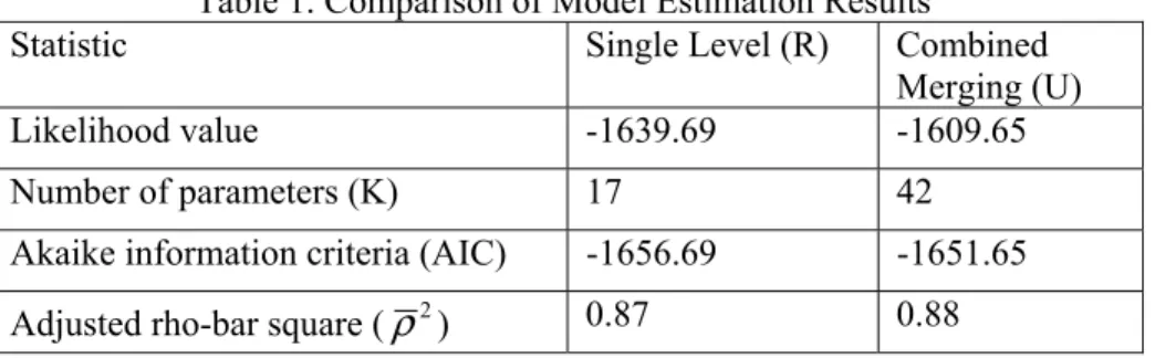
To demonstrate the usefulness of inclusion of the latent plans, the estimation results were compared against a reduced form model with no latent tactics ( Lee 2006, Choudhury et al. 2007a). In the reduced form model, gap acceptance was modeled as an instantaneous single level decision that assumes the same critical gaps for normal, courtesy, and forced merging. The statistical comparison results are presented in Table 1.
Statistical tests indicated that the latent plan model has a significantly better goodness-of-fit compared to the reduced form model.
Table 1. Comparison of Model Estimation Results
Statistic Single Level (R) Combined
Merging (U)
Likelihood value -1639.69 -1609.65
Number of parameters (K) 17 42
Akaike information criteria (AIC) -1656.69 -1651.65
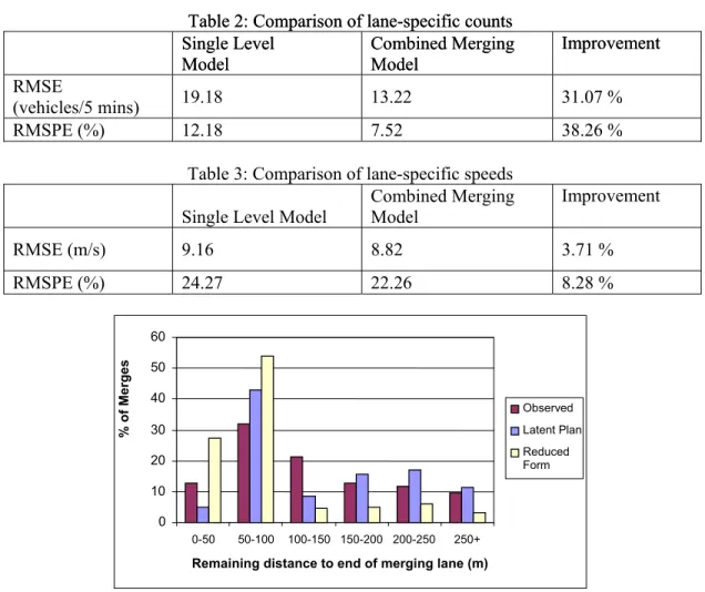
Both models were implemented in the microscopic traffic simulator MITSIMLab (Yang and Koutsopoulos 1996) and the performances in replicating traffic were compared in a different location using data from US 101, CA (Cambridge Systematics 2005). Different behavioural components of the traffic simulator were jointly calibrated using aggregate data collected from this site. A different set of aggregate data (not used for aggregate calibration) were used for validation purposes. The following measures of effectiveness were used in this regard:
Both models were implemented in the microscopic traffic simulator MITSIMLab (Yang and Koutsopoulos 1996) and the performances in replicating traffic were compared in a different location using data from US 101, CA (Cambridge Systematics 2005). Different behavioural components of the traffic simulator were jointly calibrated using aggregate data collected from this site. A different set of aggregate data (not used for aggregate calibration) were used for validation purposes. The following measures of effectiveness were used in this regard:
• Lane-specific flows • Lane-specific flows • Lane-specific speeds • Lane-specific speeds • Location of merges • Location of merges
The results are summarized in Tables 2 and 3 and Figure 7. The results are summarized in Tables 2 and 3 and Figure 7.
As seen in the tables and figure, the latent plan model was found to consistently perform better than the reduced model in simulating the observed traffic characteristics and had a much better representation of the actual congestion (Choudhury 2007, Choudhury et al. 2007b).
As seen in the tables and figure, the latent plan model was found to consistently perform better than the reduced model in simulating the observed traffic characteristics and had a much better representation of the actual congestion (Choudhury 2007, Choudhury et al. 2007b).
Table 2: Comparison of lane-specific counts Table 2: Comparison of lane-specific counts
Single Level Single Level
Model Model Combined Merging Combined Merging Model Model Improvement Improvement RMSE (vehicles/5 mins) 19.18 13.22 31.07 % RMSPE (%) 12.18 7.52 38.26 %
Table 3: Comparison of lane-specific speeds Single Level Model
Combined Merging Model Improvement RMSE (m/s) 9.16 8.82 3.71 % RMSPE (%) 24.27 22.26 8.28 % Figure 7: Comparison of location of merges
0 10 20 30 40 50 60 0-50 50-100 100-150 150-200 200-250 250+
Remaining distance to end of merging lane (m)
% of Merges Observed Latent Plan Reduced Form 66
6 Conclusion
A general methodology and framework for modelling behaviours with unobserved or latent plans has been presented in this paper. The action at any time depends on the plan at that time. In dynamic contexts, the current plan can also depend on previous plans and actions as well as attributes of different plans, expected utilities of executing the plans and the characteristics of the individual. The computational tractability of the state dependent model is attained by using the HMM approach. Using the HMM principles, the modelling assumption reduces to the following: the current action only depends on the current plan; the current plan depends only on the previous plan.
The justifications for using the latent plan modeling approach are further strengthened by validation case studies using aggregate traffic data within the microscopic traffic simulator MITSIMLab (Yang and Kousopoulos 1996), where the simulation capabilities of the latent plan models have been compared against the performance of the ‘reduced form’ models. In all cases, the latent plan models better replicate the observed traffic conditions.
The concept of latent plan and the proposed framework have enormous potential in improving behavioural models in many other travel and mobility choice applications involving dynamically evolving ‘hidden’ decision layers and latent alternatives. Examples include residential location choice, route choice, shopping destination choice, activity participation, and travel behaviour models. The extent of the effect of latent planning on observed actions can however vary depending on the nature of choice situation and associated decision making. Application of the methodology in more diverse applications will therefore further validate the findings.
It may be noted that the loss of accuracy due to the HMM assumption (i.e. the plan at a given time period depends only on the plan of the previous time period; the current action depends only on the current plan) has not been tested in this application due to computational complexity. This may be evaluated in future research with a small subset of the dataset to further support the methodology. Another important direction of future research is to compare the methodology with a partially observable discrete Markov decision process (POMDP) where evaluation of optimal policies based on rational expectations is explicitly taken into account.
Acknowledgement
This paper is based upon work supported by the Federal Highway Administration under contract number DTFH61-02-C-00036. Any opinions, findings and conclusions or recommendations expressed in this publication are those of the authors and do not necessarily reflect the views of the Federal Highway Administration.
68
References
Adams, P., Hurd, M., McFadden, D., Merrill, A. and Ribeiro, T. 2003. Healthy, wealthy and
wise? Tests for direct causal path between health and socioeconomic status, Journal of
Econometrics, 112(1) 3-56.
Alexiadis, V., Gettman, D., and Hranac, R. 2004. NGSIM Task D: Identification and Prioritization of Core Algorithm Categories, Federal Highway Administration, FHWA-HOP-06-008.
Aptech Systems, 2003. GAUSS Manual, Volume I and II, Maple Valley, WA.
Astrom, K. J., 1965. Optimal control of Markov decision processes with incomplete state
estimation, Journal of Mathematical Analysis and Applications, 10(1), 174-205.
Baker, J. K., 1975. The dragon system-An overview, IEEE Trans, Acoustic, Speech and Signal
Processing, ASSP-23-1, 24-29.
Barto, A., Bradtke, S. and Singh, S., 1995. Learning to act using real-time dynamic
programming, Artificial Intelligence, Special Volume on Computational Research on
Interaction and Agency, 72(1) 81-138.
Baum, L. E. and Petrie, T. P., 1966. Statistical inference for probabilistic functions of finite state
Markov chains, Annals of Mathematical Statistics, 37(6), 1554-1563.
Baum, L. E., 1972. An inequality and associated maximization technique in statistical estimation
for probabilistic functions of Markov processes, Inequalities, 3, 1-8.
Bellman, R. E., 1957. A Markovian Decision Process, Journal of Mathematics and Mechanics,
6, 679-684.
Ben-Akiva, M., Abou-Zeid, M. and Choudhury, C., 2007. Hybrid choice models: from static to dynamic, paper presented at the Triennial Symposium on Transportation Analysis VI, Phuket, Thailand.
Ben-Akiva, M., Choudhury, C. and Toledo, T., 2006. Modeling latent choices: application to
driving behavior, paper presented at the 11th International Conference on Travel Behaviour
Research, Kyoto, Japan.
Bilmes, J., 2002. What HMMs can do, University of Washington Technical Report, https://www.ee.washington.edu/techsite/papers/documents/UWEETR-2002-0003.pdf
Blythe, J., 1999. An overview of planning under uncertainty, AI Magazine, 20(2), Summer 1999,
37–54.
Boutilier, C., Dean, T. and Hanks, S., 1999. Decision-theoretic planning: structural assumptions
and computational leverage, Journal of Artificial Intelligence Research, 11(1), 1-94.
Boutilier C., Dearden, R. and Goldszmidt, M., 1995. Exploiting structure in policy construction, in Proceedings of the Fourteenth International Joint Conference on Artificial Intelligence, Montreal, Canada, 1104-1111.
Cambridge Systematics, Inc., 2004. NGSIM: I-80 Data Analysis. http://www.ngsim.fhwa.dot.gov/
Cambridge Systematics, Inc., 2005. NGSIM: U.S. 101 Data Analysis. http://www.ngsim.fhwa.dot.gov
Chapin, F. S. Jr., 1974. Human Activity Patterns in the City: Things People Do in Time and
Space, John Wiley and Sons, New York.
Choudhury, C. 2007. Modeling Driving Decisions with Latent Plans, Ph.D. Dissertation,
Department of Civil and Environmental Engineering, MIT.
Choudhury, C., Ben-Akiva, M., Toledo, T., Lee, G. and Rao, A., 2007. Modeling cooperative
lane-changing and forced merging behavior, paper presented at the 86th Transportation
Research Board Annual Meeting, Washington DC, USA.
Choudhury, C., Ben-Akiva, M., Toledo, T., Rao, A. and Lee, G., 2007. Modeling
state-dependence in lane-changing behavior, paper presented at the 17th International Symposium
69
Dean, T., Kaelbling, L., Kirman, J. and Nicholson, A., 1995. Planning under time constraints in
stochastic domains, Artificial Intelligence, 76(1-2), 3-74.
Dearden, R. and Boutilier, C., 1994. Integrating planning and execution in stochastic domains, in Proceedings of the Tenth Conference on Uncertainty in Artificial Intelligence, Washington, DC, 162-169.
Feldman, J. A. and Sproull, R. F., 1977. Decision theory and artificial intelligence ii: The hungry monkey, Cognitive Science, 1(2), 158–192.
Jelinek, F., 1976. Continuous speech recognition by statistical methods, in Proceedings of IEEE,
64, 532-536.
Koski, T., 2001. Hidden Markov Models for Bioinformatics, Kluwer, Dordrecht.
Kushmerick, N., Hanks, S. and Weld, D. S., 1994. An algorithm for probabilistic
least-commitment planning, in Proceedings AAAI-94, Seattle, WA, 1073- 1078.
Lee, G., 2006. Modeling Gap Acceptance at Freeway Merges, M.S. Thesis, Department of Civil
and Environmental Engineering, MIT.
Loewenstein, G. and Angner, E., 2003. Predicting and indulging changing preferences, in Time
and Decision: Economic and Psychological Perspectives on Intertemporal Choice, Loewenstein, G., D. Read, and R. Baumeister (eds.), 351-391, Russell Sage Foundation, New York.
Luenberger, D. G., 1973. Introduction to Linear and Nonlinear Programming, Addison-Wesley, Reading, Massachusetts.
Mahmassani, H. S. and Liu, Y., 1999. Dynamics of commuting decision behaviour under
advanced traveller information systems, Transportation Research Part C, 7(2-3), 91-107.
McGinnis, R., 1968. A stochastic model of social mobility, American Sociological Review,
33(5), 712-722.
Neal, D. T., Wood, W. and Quinn, J. M., 2006. Habits – a repeat performance, Current
Directions in Psychological Science, 15(4), 198-202.
Peot, M. A. and Smith, D. E., 1992. Conditional nonlinear planning, in Proceedings of the First
International Conference on Artificial Intelligence Planning Systems, 189–197.
Rabiner, L. R., 1989. A tutorial on Hidden Markov Models and selected applications in speech
recognition, in Proceedings of the IEEE, 257-286.
Rao, A., 2006. Modeling Anticipatory Driving Behavior, M.S. Thesis, Department of Civil and
Environmental Engineering, MIT.
Redelmeier, D. A., Katz, J. and Kahneman, D., 2003. Memories of colonoscopy: a randomized trial, Pain, 104(1-2), 187-194.
Ribeiro, T., 2004. Hidden Markov models and their applications to estimation, forecasting and
policy analysis in panel data settings, Working paper.
Simmons, R. and Koenig, S., 1995. Probabilistic robot navigation in partially observable
environments, in Proceedings of the Fourteenth International Joint Conference on Artificial
Intelligence, Montreal, Canada, 1080-1087.
Smallwood, R. D. and Sondik, E. J., 1973. The optimal control of partially observable Markov
processes over a finite horizon, Operations Research, 21(5) (Sep. - Oct., 1973), 1071-1088.
Strotz, R. H., 1955-56. Myopia and Inconsistency in Dynamic Utility Maximization, Review of Economic Studies, 23(3), 165—180.
Tash, J. and Russell, S., 1994. Control strategies for a stochastic planner, in Proceedings of the Twelfth National Conference on Artificial Intelligence, Seattle, WA, 1079-1085.
Verplanken, B., Aarts, H., van Knippenberg, A. and Moonen, A., 1998. Habit versus planned
behaviour: a field experiment, The British Journal of Social Psychology, 37(1), 111-128.
Vogel, S., Ney, H. and Tilmann, C., 1996. HMM-based word alignment in statistical translation, in Proceedings of the 16th Conference on Computational Linguistics, 2, 836-841.
70
Wooldridge, J. M., 2005. Simple solutions to the initial conditions problem in dynamic
non-linear panel data models with unobserved heterogeneity, Journal of Applied Econometrics,
20, 39-54.
Yang, Q. and Koutsopoulos, H. N., 1996. A microscopic traffic simulator for evaluation of