HAL Id: hal-01868457
https://hal.archives-ouvertes.fr/hal-01868457
Submitted on 5 Sep 2018
HAL is a multi-disciplinary open access
archive for the deposit and dissemination of
sci-entific research documents, whether they are
pub-lished or not. The documents may come from
teaching and research institutions in France or
abroad, or from public or private research centers.
L’archive ouverte pluridisciplinaire HAL, est
destinée au dépôt et à la diffusion de documents
scientifiques de niveau recherche, publiés ou non,
émanant des établissements d’enseignement et de
recherche français ou étrangers, des laboratoires
publics ou privés.
Stress Estimation in Reservoirs by a Stochastic Inverse
Approach
Antoine Mazuyer, Richard Giot, Paul Cupillard, Marianne Conin, Pierre
Thore
To cite this version:
Antoine Mazuyer, Richard Giot, Paul Cupillard, Marianne Conin, Pierre Thore. Stress Estimation in
Reservoirs by a Stochastic Inverse Approach. 7th International Symposium on In-Situ Rock Stress,
May 2016, Tampere, Finland. �hal-01868457�
STRESS ESTIMATION IN RESERVOIRS BY A STOCHASTIC INVERSE APPROACH
Antoine Mazuyer ([email protected])
Université de Lorraine – GeoRessources – RING Team France
Richard Giot
Université de Lorraine – GeoRessource France
Paul Cupillard
Université de Lorraine – GeoRessources – RING Team France
Marianne Conin
Université de Lorraine – GeoRessources France
Pierre Thore Total SA, Pau
France
ABSTRACT
The aim of this study is to estimate the initial stress in reservoirs before production using 3D calibrated geomechanical models. We propose an inverse method for estimating stress. Wellbore data can be integrated in a Mechanical Earth Model in order to estimate stresses nearby wells. It yields a first rough estimation in the whole reservoir by a simple interpolation which is not in equilibrium with the external forces and boundary conditions. From this rough stress field, the inversion aims at finding a physically acceptable stress state (i.e.: in equilibrium with the external forces and boundary conditions) that fit the local stresses wells. The forward problem is ensured by a Finite Element Analysis which is able to take into account structures such as faults, which have a significant influence on the stress magnitude and orientation. Inverse loop stops when the stress computed near wells matches the one estimated using borehole data. The uncertainties on the boundary conditions, elastic parameters and the first stress estimation are taken into account with a stochastic approach. In this study, faults are built with a volumetric representation of the core and damage zone by introducing elastic parameters variations within. This representation is possible because only small deformations are expected.
KEYWORDS
Stress estimation, reservoirs, elasticity, inverse problem, stochastic
INTRODUCTION
Subsoil raw materials exploitation generally induces stress changes. For instance, depletion disturbs the mechanical equilibrium, yielding a stress change in the reservoir and in the overlying geological layers (the overburden). It could have dramatic consequences such as borehole instability (Zoback et al., 2003) and fault reactivation, which can lead to unexpected oil and gas leaks or migration (Wiprut and Zoback, 2002).
Stress estimation is important during field exploitation to avoid these problems and to anticipate measures to stabilize wells using different drilling and casing techniques (Wilson et al., 1999). Depletion can be monitored and it is possible to estimate the relative stress change during the exploitation. The goal of this paper is to introduce a new approach to estimate the absolute stress in the reservoir and the overburden before
exploitation. Stress estimation needs a complete understanding of the mechanics of the reservoir. It goes through a geomechanical model building, with behaviour laws, mechanical parameters and geometric structures. Exploration wells could provide very local stress information using which are not sufficient to estimate the stress state in the whole reservoir and overburden because subsoil is often heterogeneous with different faulted and folded materials. These structures affect the stress field depending on the material mechanical properties. A simple interpolation between wells will not take into account these effects. Moreover, material properties, position and orientation of faults and horizons are prone to a lot of uncertainties. This paper presents an inverse method to estimate the stress field in the whole reservoir, in 3D geomechanical models. This method uses the Finite Element Method to compute a physically admissible stress state in the whole reservoir, consistent with both the local estimation nearby wells and the reservoir geology.
INVERSE PROBLEMS NOMENCLATURE
In mechanics, one can use a numerical model to predict a result (i.e. displacements, strain or stress fields) from given behaviour law, constitutive parameters, initial and boundary conditions. Such a problem is called the
forward problem. We use the nomenclature introduced by Tarantola, (2005) to set the inverse problem in this
paper.
)
(m
g
d
(1) m stands for the set of the model parameters (i.e. constitutive parameters, boundary and initial
conditions etc.). m belongs to the model space which can contain different models m.
d stands for the set of the observable data parameters (i.e. stress). d belongs to the data space.
g stands for the transformation, linking m and d. It can represent an analytical solution or a numerical
simulation.
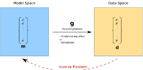
Figure 1 shows a simple scheme of the data and the model spaces.
Figure 1. Relation between the model space and the data space. m is one possible model from the model space.
d is a set of observable data parameters that can be compared to some results from the transformation g.
The inverse problem consists in using observed data to infer the model parameters (Tarantola, 2005). This paper sets the inverse problems that we want to solve in order to estimate the stress state in the whole reservoir.
FORWARD PROBLEM PRESENTATION Classical mechanical problem formulation
Stress computation in a geological model can be described as a boundary value problem (Figure 2) involving both boundary conditions and equilibrium equation.
boundary
on t he
boundary
on t he
domain
in t he
0
, h i j ij q i i i i ijh
n
q
u
F
(2)Where Fi are the external forces, qi is a prescribed boundary displacement function (Dirichlet condition) and hi is
a prescribed boundary stress function (Neumann condition). To solve this system, we have to input a constitutive behaviour law and initial and boundary conditions. The set of mechanical parameters and initial and boundary conditions describes a geomechanical model. In our case, a model from the model space will be a set of mechanical parameters and boundary conditions. The dimension of the space will be constrained by the discretization of the model in elements.
Figure 2. a) the boundary-value problem represented in a classical way (modified from Hughes 2012). b) a simple geological model. It can be also assimilated as a boundary value problem.
Because we are dealing with a boundary value problem, the Finite Element Analysis is suitable to find a solution for the system (2). The Finite Element Analysis represents the g transformation described in equation (1).
Eventually, the observable data parameters can be displacements, strains and even stresses. These parameters are punctually observed (for instance nearby well, see next section) and will be compared to the results of the g transformations of m to solve the inverse problem.
Using a linear elastic behaviour law
Linear elastic law is used to model a mechanical behaviour when no non-linearity and small deformation are expected. Indeed, we will see in the next section that we are dealing with problems involving small deformations. Moreover, running simulations on large stochastic inverse problems induces high computation costs. Using an elastic behaviour law yields to fast computations and involves few parameters to invert. This allows saving time in a first approach.
The main problem of this assumption is related to the presence of faults. In mechanics, faults are classically modeled with a friction law that makes the problem non-linear. At low stress, before failure occurs, we can assume that faults deform elastically while impacting the state of stress. It is yet reasonable to investigate the possibility of modelling faults with an elastic model, for a certain range of stress.
Faults are complex geological structures that localize the brittle deformation of the upper crust. They are often defined as an ensemble of a fault core and a damage zone (Figure 3) (Torabi and Berg, 2011). The fault core is where the deformations and the displacements are the highest. The damage zone surrounds the fault core ; it is made of brittle rocks with a high density of fractures (Torabi and Berg, 2011). Faulkner et al., (2006), carried experimental laboratory work to determine the mechanical properties in the fault damage zone using microfracture density. They show that the elastic properties vary as a function of the distance from the fault core: Young modulus increases with distance from the fault core, whereas the Poisson's ratio decreases, because the material becomes more brittle near the fault core. The authors then developed a model to compute stress in a horizontal plane cutting a fault. A stress σ1 is applied on the boundaries with different angles with the fault. Mean
stress value increases from the edge of the damage zone to the fault core, which shows a stress accumulation occurring nearby faults.
Figure 3. Simple scheme of a fault with its fault core and its damage zones.
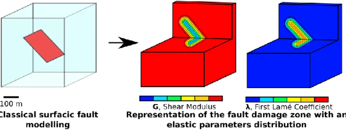
From these observations, we develop a 3D elastic model of the faults. Classically, in geomodellers, faults are modelled with a surface. We assume that this surface is the fault core and we introduce an elastic parameters distribution in the fault damage zone: the shear modulus is decreasing from the edge of the damage zone to the fault core as the first Lame coefficient increasing. With these kinds of elastic parameters variations, we assume that the shear is the highest nearby the fault core (Figure 4).
Figure 4. Classical surfacic fault modelling VS volumic fault modelling using elastic parameters distribution function of the distance to the fault.
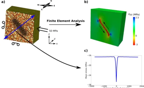
In order to see if this approach produces suitable stress variation nearby the faults, we run a simple Finite Element Analysis on the model presented on Figure 4 by reproducing a compressive context. Figure 5 presents the boundary conditions applied on the model and the results. To run the Finite Element Analysis, we use a homemade library based on the open-source mesh library RINGMesh1. This let us the possibility to set the elastic parameters different on each cells in order to reproduce the distribution shown in Figure 4. σzz shows
symmetric compressive and extensive quadrants. These quadrants are consistent with the reverse fault regime expected. The magnitude of the mean stress increases from the edge of the damage zone to the fault core, which is coherent with the Faulkner observations.
Figure 5. a). The model is meshed using extrusion method from the fault (Renaudeau et al., 2015): it is refined on the damage zone, where the elastic parameters are changing. Neumann condition of 50 MPa is applied on
the East face of the model. Displacement is set to zero in x direction on the West face, in z direction on the Bottom face, and in y direction on the North face. b) σzz computation shows anti-symmetric compressive and
extensive quadrants. c) Mean stress magnitude evolution on a line perpendicular to the fault.
Sign convention is: compressive stress as negative.
This approach may not be sufficient when the mechanical behaviour nearby the fault is not elastic despite of the small deformation hypothesis. Perspectives of this study are to introduce other parameters describing locally the elasto-plastic behaviour (i.e. Hoek and Brown criterion (Hoek and Brown, 1980), nearby the fault core or in the damage zone). An alternative would be to represent a fault zone as a single surface, through interface elements with a friction law, such as Coulomb’s.
STRESS ESTIMATION NEARBY WELLBORE
Drilling wells bring information about the encountered materials. They can be equipped with logging tools to infer stresses nearby wells. Petroleum industry gives a lot of attention on borehole stability. As a consequence, the geomechanics nearby wells needs to be fully understood. Mechanical Earth Models are numerical representations of the stress field nearby the wells. They are 1D models compounded of depth profiles of elasto-plastic parameters. These models generally assume that the vertical stress (denoted σv) is one of the principal
stresses, so that the maximum horizontal stress and the minimum principal stress (respectively σhmin σHmax) are
the two other principal stresses. So σv, σhmin, and σHmax can be estimated nearby the boreholes using this model.
The reader may refer to Plumb et al. (2000) to find more information about this widely used mechanical model. Stress estimation nearby the wells will be used in the inverse problem as the observable data parameters (see next section).
GLOBAL STRESS INVERSION
We assume that the studied reservoir and overburden are in a mechanical equilibrium. It means that the external forces that apply on the boundaries of the domain are in equilibrium with the internal stress. To compute this stress, a rough estimation is first done in the whole reservoir and the overburden (e.g. a stress estimation using
the rock weight and a simple interpolation between the stresses estimated on the wells). This stress state is not in equilibrium with the external forces corresponding to the regional tectonic context, so it needs to be changed until it reaches equilibrium with the boundary conditions. However there are uncertainties on the elastic parameters and on the boundary conditions. Therefore, a stochastic approach is planned in order to deal with these uncertainties. Inputs of the forward problem will be a set of models (m = {m1, m2,…,mn
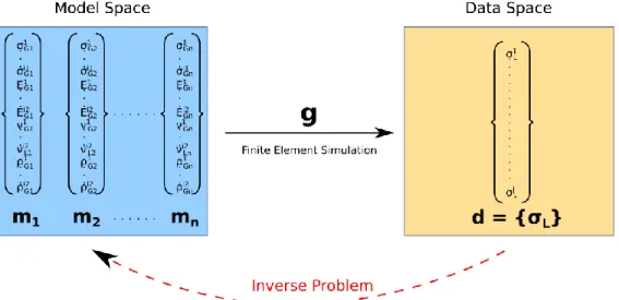
}) corresponding to different combinations of elastic parameters and boundary conditions. One way to deal with these different set of models with a large number of variables is to use ensemble inverse method such as CMA-ES (Hansen and Ostermeier, 2001) which is an evolutionary algorithm based on a stochastic method for optimization problems. A population is represented by the set of models. This population evolves until a cost function is minimized. Finite Element Analysis is used as the g transformation to compute the equilibrium state on each model. It will handle the effect of the structures on the stress. The result of the simulations gives a physically admissible stress state. We are not taking into account the whole geological history because it would be tedious to integrate in the inversion process. We made the assumption that the mechanical evolution to the equilibrium follows an elastic behaviour, except nearby some faults where we assume a plastic behaviour. Indeed, we expect small deformation during the evolution from the rough stress estimation to the equilibrium state. Moreover, using an elastic behaviour law yields to fast computation. This is an important parameter when dealing with stochastic simulations with a lot of realisations. As a consequence, the model space contains models with the different mechanical parameters (elastic or elasto-plastic) and the boundary conditions. Stress estimated using the Mechanical Earth Model will be used as the set of observable data parameters in the inverse problem (see Figure 6).
Figure 6. Scheme of the inverse problem. The model space contains all the models mi generated for the
simulation. It let us handle the uncertainties. In this scheme, it contains only models with a full elastic behaviour. G subscript stands for Global because these are models at the reservoir scales. The data space contains all the obserable data which are the local stress estimation from the Mechanical Earth Model. L subscript stands for
Local because these are local data obtained nearby wells.
In practice, a sensibility study of the models parameters on the forward problem will be done to select which one are relevant to invert. The parameters which have the more influence on the results will be kept. In a first approach, the mechanical parameters can be fixed and the model space will contain only sets of boundary conditions.
CONCLUSIONS
We see in this article that the problem of stress computation is multiscale, which makes it difficult to model. Using the Mechanical Earth Model let us taking into account the data provided by the wells to estimate the stresses locally. This information is used as data for the inversion. This change of scale raises the problem of upscalling.
Uncertainties on the model parameters (mechanical parameters and boundary conditions) are taken into account using stochastic approach to use a set of models instead of one unique model.
A linear elastic law is preferred as a first approach. It leads to the discussion about the fault mechanical modelling. We have found that using only elastic parameters on the fault damage zone yields to consistent results. The perspectives of this study on mechanical fault modelling are to analyse these results quantitatively and to compare them with other behaviour law (plastic, elasto-plastic or friction law).
ACKNOWLEDGEMENTS
This work was performed in the frame of the RING project at Université de Lorraine. We would like to thank the industrial and academic sponsors of the Gocad Research Consortium managed by ASGA for their support, in particular Total for additional support for Antoine Mazuyer Ph.D.
REFERENCES
Faulkner, D. R., Mitchell, T. M., Healy, D., and Heap, M. J. Slip on 'weak' faults by the rotation of regional stress
in the fracture damage zone. Nature 444.7121 (2006): 922-925.
Hansen, N. and A. Ostermeier. Completely Derandomized Self-Adaptation in Evolution Strategies. Evolutionary Computation, (2001), 9(2), pp. 159-195
Hoek, E., and Brown E. T. Underground excavations in rock. No. Monograph. 1980.
Hughes, Thomas JR. The finite element method: linear static and dynamic finite element analysis. Courier Corporation, 2012.
Plumb, Richard A., and Stephen H. Hickman. Stress‐induced borehole elongation: A comparison between the four‐arm dipmeter and the borehole televiewer in the Auburn Geothermal Well. Journal of Geophysical
Research: Solid Earth (1978–2012) 90.B7 (1985): 5513-5521.
Kirsch, Gustav. Die theorie der elastizität und die bedürfnisse der festigkeitslehre. Springer, 1898.
Plumb, R., Edwards, S., Pidcock, G., Lee, D., and Stacey, B.. The mechanical earth model concept and its
application to high-risk well construction projects. IADC/SPE Drilling Conference. Society of Petroleum
Engineers. (2000)
Renaudeau, J., Botella, A, Caumon, G, Levy, B. Tetrahedral and hex-dominant meshing for fault damage zones. 35th Gocad Meeting - 2015 RING Meeting., 2015
Tarantola, Albert. Inverse problem theory and methods for model parameter estimation. siam, 2005.
Torabi, A. and Silje S. Scaling of fault attributes: a review. Marine and Petroleum Geology 28.8 (2011): 1444-1460.
Willson, S. M., Last, N. C., Zoback, M. D., and Moos, D. Drilling in South America: a wellbore stability approach
for complex geologic conditions. Latin American and Caribbean petroleum engineering conference. Society of
Petroleum Engineers, 1999.
Wiprut, David and Mark D. Zoback. Fault reactivation, leakage potential, and hydrocarbon column heights in the
northern North Sea. Norwegian Petroleum Society Special Publications 11 (2002): 203-219.
Zoback, M. D., Barton, C. A., Brudy, M., Castillo, D. A., Finkbeiner, T., Grollimund, B. R, Wiprut, D. J.
Determination of stress orientation and magnitude in deep wells. International Journal of Rock Mechanics and