Fast computation of the geoelectric field using the method of elementary current systems and planar Earth models

HAL Id: hal-00317211

https://hal.archives-ouvertes.fr/hal-00317211

Submitted on 1 Jan 2004

HAL is a multi-disciplinary open access

archive for the deposit and dissemination of

sci-entific research documents, whether they are

pub-lished or not. The documents may come from

teaching and research institutions in France or

abroad, or from public or private research centers.

L’archive ouverte pluridisciplinaire HAL, est

destinée au dépôt et à la diffusion de documents

scientifiques de niveau recherche, publiés ou non,

émanant des établissements d’enseignement et de

recherche français ou étrangers, des laboratoires

publics ou privés.

Fast computation of the geoelectric field using the

method of elementary current systems and planar Earth

models

A. Viljanen, A. Pulkkinen, O. Amm, R. Pirjola, T. Korja

To cite this version:

A. Viljanen, A. Pulkkinen, O. Amm, R. Pirjola, T. Korja. Fast computation of the geoelectric field

using the method of elementary current systems and planar Earth models. Annales Geophysicae,

European Geosciences Union, 2004, 22 (1), pp.101-113. �hal-00317211�

Annales Geophysicae (2004) 22: 101–113 © European Geosciences Union 2004

Annales

Geophysicae

Fast computation of the geoelectric field using the method of

elementary current systems and planar Earth models

A. Viljanen1, A. Pulkkinen1, O. Amm1, R. Pirjola1, T. Korja2,*, and BEAR Working Group3

1_{Finnish Meteorological Institute, Geophysical Research Division, P.O.B. 503, FIN-00101 Helsinki, Finland} 2_{Geological Survey of Finland, P.O.B. 96, FIN-02151 Espoo, Finland}

3_{Contact person: T. Korja}

*_{now at: University of Oulu, Department of Geosciences, P.O.B. 3000, FIN-90014 Oulu, Finland}

Received: 25 October 2002 – Revised: 3 June 2003 – Accepted: 18 June 2003 – Published: 1 January 2004

Abstract. The method of spherical elementary current

sys-tems provides an accurate modelling of the horizontal com-ponent of the geomagnetic variation field. The interpolated magnetic field is used as input to calculate the horizontal geoelectric field. We use planar layered (1-D) models of the Earth’s conductivity, and assume that the electric field is re-lated to the local magnetic field by the plane wave surface impedance. There are locations in which the conductivity structure can be approximated by a 1-D model, as demon-strated with the measurements of the Baltic Electromagnetic Array Research project. To calculate geomagnetically in-duced currents (GIC), we need the spatially integrated elec-tric field typically in a length scale of 100 km. We show that then the spatial variation of the electric field can be neglected if we use the measured or interpolated magnetic field at the site of interest. In other words, even the simple plane wave model is fairly accurate for GIC purposes. Investigating GIC in the Finnish high-voltage power system and in the natural gas pipeline, we find a good agreement between modelled and measured values, with relative errors less than 30% for large GIC values.

Key words. Geomagnetism and paleomagnetism

(geomag-netic induction; rapid time variations) – Ionosphere (electric field and currents)

1 Introduction

Temporal variations of the geomagnetic field are accompa-nied by an electric field whose horizontal component can, in extreme cases, exceed 10 V/km at the Earth’s surface. The geoelectric field produces currents in the conducting Earth as well as in manmade conductors such as power systems and pipelines. In the case of technological systems, the term geomagnetically induced current (GIC) is used. GICs are of practical importance due to possibly harmful effects (Bolduc, 2002; Boteler et al., 1998; Gummow, 2002;

Kap-Correspondence to: A. Viljanen (ari.viljanen@fmi.fi)

penman, 1996; Lahtinen and Elovaara, 2002; Lesher et al., 1994; Molinski, 2002; Osella et al., 1998; Pirjola et al., 2002). Only few really severe GIC disturbances have oc-curred, but developing methods for calculating the geoelec-tric field is relevant as basic research, too: a successful mod-elling of GIC requires a detailed knowledge of ionospheric currents and of the Earth’s conductivity, and provides a com-prehensive test for geospace models.

The calculation of GIC in a conductor system consists of two independent steps: determination of the geoelectric field, and computation of GIC due to the given electric field. The latter task is different for discretely (e.g. power grids; see Lehtinen and Pirjola, 1985) and continuously grounded systems (e.g. buried pipelines; see Pulkkinen et al., 2001a; Trichtchenko and Boteler, 2002), but it is simple compared to the former part. The difficulty in the geophysical step arises from the fact that GIC is not only affected by spatially and temporally complicated ionospheric currents, but the geo-electric field also crucially depends on the Earth’s conductiv-ity. In this sense the electric field differs from the magnetic field, because the latter can be fairly accurately calculated without taking into account induction effects (cf. Tanskanen et al., 2001).

The calculation of the geoelectric field requires that iono-spheric currents are known as functions of time and space, and that a model of the Earth’s conductivity is known. In practice, a full 3-D modelling of the whole geospace is not feasible. The knowledge of the ionosphere and the Earth is never perfect either. In GIC studies it is not necessary to know the spatial structure of the electric field in a kilome-tre scale. When GIC is determined in a power system or a pipeline, the electric field is integrated along the conductors. Consequently, the relevant spatial scale is given, for example, by the distances between nodes of a power system, which are at least tens of kilometres in Finland. Consequently, regional averages of the field are adequate for GIC purposes.

A sophisticated computation technique with layered con-ductivity structures is the complex image method (CIM) (Lindell et al., 2000; Thomson and Weaver, 1975; Wait and

102 A. Viljanen et al.: Fast computation of the geoelectric field Spies, 1969), which, in a generalised form, allows for

in-cluding realistic 3-D models of ionospheric currents (Pirjola and Viljanen, 1998). It allows for use of closed-form for-mulas, thus making computations much faster than with the exact Fourier integrals. Viljanen et al. (1999a) and Vilja-nen et al. (1999b) applied this technique to models of typical ionospheric events in order to investigate the magnetotelluric source effect, and to calculate GIC in the Finnish power grid. A major advantage in the modelling of the ionosphere is the method of spherical elementary current systems (SECS) (Amm and Viljanen, 1999; Pulkkinen et al., 2003a,b). It al-lows for rapid determination of equivalent ionospheric cur-rents from regional to global scales. The combination of CIM and SECS was introduced by Pulkkinen et al. (2003a), and we now demonstrate its applicability of determining the geo-electric field for GIC calculations. Although CIM is a con-venient tool for theoretical modelling purposes, it is not the most optimal choice for more operational applications. As a replacement, we show that a simple local 1-D assumption is very reasonable when we aim at calculating the spatially av-eraged geoelectric field from the magnetic field determined with SECS. So we can calculate the electric field at any sur-face point with a different 1-D conductivity model at each site if desired, and then numerically integrate the field along conductors to obtain the GIC. We also show that even the simplest plane wave method with spatially uniform fields is good enough in GIC calculations, on the important condition that the magnetic field used is measured close to or interpo-lated at the GIC site under study. A further advantage in the plane wave method is that GIC is directly determined by the horizontal electric field via constant multipliers without the need to integrate the field separately for each time step.

We present a strict physical approach, which starts from geomagnetic recordings and provides the geoelectric field at any point at the Earth’s surface. Our method is well suited to post-analysis of interesting events. In addition, it would be useful for predicting the geoelectric field, provided that fore-casts of ground magnetic field variations are available. Al-though this paper focuses on the methodology, it also shows how complicated the geometry of the geoelectric field is and how rapidly it changes. Pulkkinen et al. (2003c) present a more detailed analysis about ionospheric currents during an extreme event.

After briefly reviewing some central equations, we first show that the assumption of a planar geometry is reason-able. Then we demonstrate that the time derivative of the ground magnetic field can be reproduced with a good accu-racy, even with quite a sparse magnetometer network. This is a critical point when considering the geoelectric field. Use-fulness of the local 1-D assumption during highly disturbed events is shown by comparing modelled and measured data of the electric field. The most important evidence is given by comparing measured and modelled GIC in the Finnish high-voltage power system and in the natural gas pipeline.

2 Method of calculation

Equivalent ionospheric currents are determined using spher-ical elementary current systems, as described by Amm and Viljanen (1999), and validated in detail by Pulkkinen et al. (2003a). The method is based on the fact that geomag-netic variations at the Earth’s surface can be explained by a horizontal divergence-free current system at the ionospheric level. Strictly speaking, induction effects in the Earth should be included by setting another current layer below the Earth’s surface, but it is omitted in this study. We are interested in highly disturbed events, where the ionospheric contribution to horizontal magnetic variations close to strong currents is typically more than 80% of the total variation (Tanskanen et al., 2001). Neglecting induction effectively means that we obtain slightly overestimated amplitudes of ionospheric equivalent currents, but the geometric patterns of the cur-rent systems remain practically unchanged. It is possible to separate the field into external and internal parts with SECS (Pulkkinen et al., 2003b), but at regions with sparse measure-ments this would not lead to a significantly better result.

We cannot determine the true 3-D ionospheric current sys-tem by using ground magnetometer data only. However, for any given 3-D system, a horizontal equivalent current system exists that produces the same magnetic and electric field at the Earth’s surface (cf. Pirjola and Viljanen, 1998). Further-more, as will be seen, we do not actually need ionospheric equivalent currents, but just the total horizontal variation field at the Earth’s surface.

Amplitudes of elementary current systems are determined by fitting the modelled horizontal field to the measured one. Although this is done in a spherical geometry, we can assume a planar geometry in local applications, which makes com-putations much simpler without affecting the modelled fields too much. Then the surface current density of an elementary system with an amplitude I at height h in cylindrical coordi-nates is (r =px2_+y2_{) is J(r) = I /(2π r) e}

φ, as given by

Amm (1997) (misprint in his formula corrected here). The electric field at the Earth’s surface due to one element is

E = −iωµ0I

4π

√

r2_+h2_−h

r eφ, (1)

where the z axis points vertically downwards, and the Earth’s surface is the xy plane, and a harmonic time-dependence (eiωt) is assumed (e.g. Pulkkinen et al., 2003a). The mag-netic field is B = µ0I 4π r ( (1 − h √ r2_+h2)er + r √ r2_+h2 ez). (2)

Because the field is calculated directly from a given current system, it automatically fulfills the Maxwell equations, es-pecially the curl-free condition of the magnetic field outside of the source region. So the SECS method provides a robust interpolation technique.

In the complex image method the effect of the Earth is approximated by setting a perfect conductor at the complex depth p(ω) = Z(ω)/(iωµ0), where Z(ω) is the plane wave

A. Viljanen et al.: Fast computation of the geoelectric field 103 surface impedance of the layered Earth defined by the

thick-nesses and electromagnetic parameters of the layers. To cal-culate the field due to induced currents in the Earth, h in Eq. (1) is replaced by h + 2p(ω), and the signs of Bzand E

are changed (corresponding to the opposite sign of the image current). So induction tends to decrease the horizontal elec-tric field and the vertical magnetic field, and to increase the horizontal magnetic field.

The simplest method to calculate the electric field from magnetic data is the local 1-D model, when

Ex(ω) = Z(ω) µ0 By(ω), Ey(ω) = − Z(ω) µ0 Bx(ω). (3)

At first sight, this may appear as a severe oversimplification, since it basically requires that the fields are laterally con-stant, which, in turn, presumes that neither the ionospheric currents, nor the Earth’s conductivity have lateral variations. However, the formula works quite well if we use local 1-D Earth models and the local magnetic field. In fact, a strict lateral constancy is not required, but a linear spatial variation of the fields is allowed (Dmitriev and Berdichevsky, 1979).

An advantage compared to CIM is that now the magnetic field provided by SECS is exactly the one needed in the lo-cal 1-D method, i.e. the total horizontal variation field at the Earth’s surface. So induction effects are not taken into ac-count twice, as in the combination of SECS and CIM, where ionospheric equivalent currents are biased by the effect of telluric currents.

3 Application to real data

3.1 Modelled and measured fields during the BEAR project Baltic Electromagnetic Array Research (BEAR) is a subpro-ject of SVEKALAPKO

(SVEcofennian-KArelia-LAPland-KOla). SVEKALAPKO is aimed to determine the

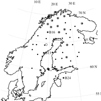
ge-ometry, thickness and age of the lithosphere, the upper-most shell of the solid Earth, and the disposition of ma-jor lithospheric structures in the Fennoscandian (Baltic) Shield (Korja et al., 2002). Within the BEAR measurement phase, June–July 1998, the magnetic and electric fields were recorded with a 2 or 10-second time resolution in a dense network in Fennoscandia (Fig. 1). In this study, we use one-minute averaged BEAR data.

The elementary current systems were placed in the iono-sphere at the height of 100 km in a regular grid, which cov-ered the continental part of IMAGE with extensions of some degrees. A typical number of grid points was around 250 in the range of 55–75 deg N and 0–35 deg long, with spacings of 1.25 deg latitudinally and 2.5 deg longitudinally.

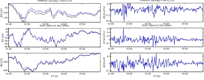
We first show that the assumption of a planar geometry is acceptable. Figure 2 depicts the calculated magnetic field in spherical and planar geometries. The amplitudes of elemen-tary current systems were determined in the spherical geom-etry. The planar geometry was then constructed by a stere-ographic projection. In particular, the good correspondence

Figures

Fig. 1. BEAR sites in summer 1998. IMAGE magnetometer stations operating at that time are marked

with circles (Svalbard excluded). The four stations B13, B16, B22, B24 used in Fig. 5 are assigned by

their codes.

black: spherical, blue: planar

01:00 02:00 03:00 04:00 05:00 -150 -100 -50 BX [nT] 19980626, (lat,long) = (60.0,22.0) 01:00 02:00 03:00 04:00 05:00 -0.5 0 0.5 UT [h] dZ/dt [nT] 01:00 02:00 03:00 04:00 05:00 -0.2 0 0.2 0.4 0.6 dY/dt [nT/s]

black: spherical, blue: planar

01:00 02:00 03:00 04:00 05:00 -0.4 -0.2 0 0.2 dX/dt [nT/s] 19980626, (lat,long) = (60.0,22.0)

Fig. 2. Comparison of the ground magnetic field and its time derivative calculated in a spherical (black

line) and planar geometry (blue line). The ionospheric equivalent current system used as input for both

cases was determined in the spherical geometry. The effect of the conducting earth is ignored.

24

Fig. 1. BEAR sites in summer 1998. IMAGE magnetometer

sta-tions operating at that time are marked with circles (Svalbard ex-cluded). The four stations B13, B16, B22, B24 used in Fig. 5 are assigned by their codes.

between the time derivative of the magnetic field is notable, since it is closely related to the geoelectric field. (The time derivative is calculated as a difference between two succes-sive field values.)

Using BEAR data, Pulkkinen et al. (2003a) showed that the SECS method reproduces the horizontal ground magnetic variation field very well, and they also demonstrated that its time derivative (dH/dt) is accurately reproduced at the mea-suring sites. We will now have a closer look at dH/dt . To show that the relatively sparse IMAGE network can yield good interpolated values of dH/dt , we consider a disturbed day of 26 June 1998. We determined equivalent currents us-ing the 14 IMAGE magnetometer stations that were operat-ing on the continent duroperat-ing that day. (Nowadays, the situa-tion is better, since there are 22 continental sites.) During an intense substorm, a westward electrojet covered the whole continental part of BEAR, as seen in Fig. 3. There are no striking features in the horizontal field pattern. On the con-trary, dH/dt is much more structured, which is typical at these latitudes (Pulkkinen et al., 2003a,c).

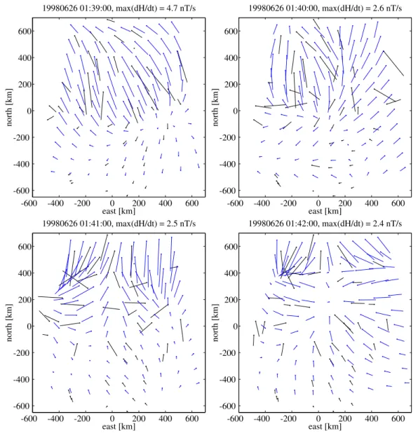
A sequence of dH/dt plots shows how rapidly the pat-terns change in a one-minute timescale (Fig. 4). The equiva-lent currents are not shown, but they are very similar to those in Fig. 3. Recalling that we used only IMAGE magnetome-ters to determine elementary currents systems, we still ob-tain a satisfactory fit even for dH/dt . There are clear devi-ations in magnitudes and direction in places, but the over-all structure is mostly well reproduced. As Pulkkinen et al. (2003a) showed, very small-scale ionospheric features (less

104 A. Viljanen et al.: Fast computation of the geoelectric field

Figures

Fig. 1. BEAR sites in summer 1998. IMAGE magnetometer stations operating at that time are marked

with circles (Svalbard excluded). The four stations B13, B16, B22, B24 used in Fig. 5 are assigned by

their codes.

black: spherical, blue: planar

01:00 02:00 03:00 04:00 05:00 -150 -100 -50 BX [nT] 19980626, (lat,long) = (60.0,22.0) 01:00 02:00 03:00 04:00 05:00 -0.5 0 0.5 UT [h] dZ/dt [nT] 01:00 02:00 03:00 04:00 05:00 -0.2 0 0.2 0.4 0.6 dY/dt [nT/s]

black: spherical, blue: planar

01:00 02:00 03:00 04:00 05:00 -0.4 -0.2 0 0.2 dX/dt [nT/s] 19980626, (lat,long) = (60.0,22.0)

Fig. 2. Comparison of the ground magnetic field and its time derivative calculated in a spherical (black

line) and planar geometry (blue line). The ionospheric equivalent current system used as input for both

cases was determined in the spherical geometry. The effect of the conducting earth is ignored.

24

Fig. 2. Comparison of the ground magnetic field and its time derivative calculated in a spherical (black line) and planar geometry (blue

line). The ionospheric equivalent current system used as input for both cases was determined in the spherical geometry. The effect of the conducting Earth is ignored.

-500

0

500

-500

0

500

east [km]

north [km]

19980626 01:47:00, max(dH/dt) = 1108 nT

-500

0

500

-500

0

500

east [km]

north [km]

max(dH/dt) = 5.3 nT/s

Fig. 3. Measured and modelled horizontal magnetic field in the BEAR region on June 26, 1998, 0147

UT. Left panel: horizontal magnetic field vectors (rotated 90 degrees clockwise). Right panel: time

derivative of the horizontal magnetic field. Measured values are shown with black arrows and modelled

with blue arrows. The effect of the conducting earth is ignored. Only IMAGE magnetometer were used

to derive ionospheric equivalent currents.

25

Fig. 3. Measured and modelled horizontal magnetic field in the BEAR region on 26 June 1998, 01:47 UT. Left panel: horizontal magnetic

field vectors (rotated 90 degrees clockwise). Right panel: time derivative of the horizontal magnetic field. Measured values are shown with black arrows and modelled with blue arrows. The effect of the conducting Earth is ignored. Only IMAGE magnetometer were used to derive ionospheric equivalent currents.

than about 100 km scale sizes) cannot be explained due to the sparsity of the ground magnetometer array, and also due to the 100 km distance from the surface to the ionosphere. It would be possible to improve the fit at measuring sites, but the price would be to allow unrealistically varying patterns between observation points.

The use of the recorded BEAR electric field is more com-plicated, because it is typically very much distorted due to local geology. However, some stations are obviously at loca-tions where a 1-D Earth model is a good approximation. We

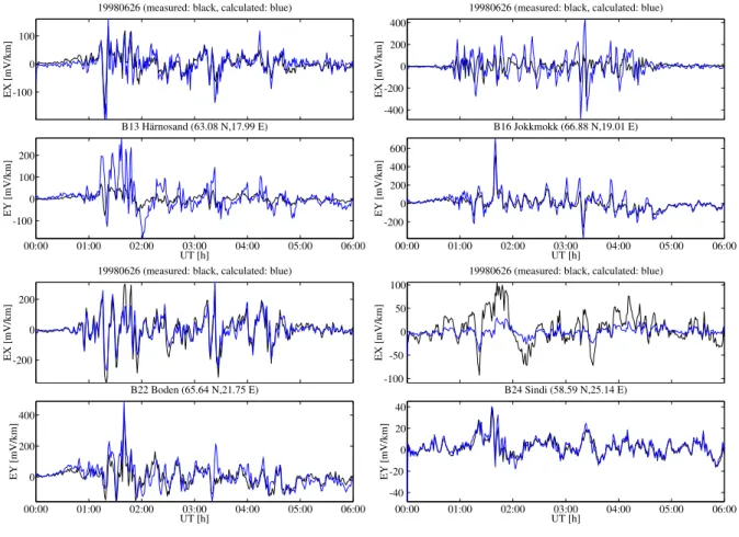
calculated the electric field using the local 1-D method with conductivity models compiled from the conductance map of the Fennoscandian Shield (Korja et al., 2002), and averaged on an area of 50 km × 50 km (Table 1). Examples of four sites at different latitudes during high magnetic activity are shown in Fig. 5. It is noteworthy how accurately the field can be modelled with the local 1-D method, although this is definitely not a plane wave event. The approximative nature of the 1-D assumption is clear, especially at B24. There are several other sites not shown here where the local 1-D model

A. Viljanen et al.: Fast computation of the geoelectric field 105 -600 -400 -200 0 200 400 600 -600 -400 -200 0 200 400 600 east [km] north [km] 19980626 01:39:00, max(dH/dt) = 4.7 nT/s -600 -400 -200 0 200 400 600 -600 -400 -200 0 200 400 600 east [km] north [km] 19980626 01:40:00, max(dH/dt) = 2.6 nT/s -600 -400 -200 0 200 400 600 -600 -400 -200 0 200 400 600 east [km] north [km] 19980626 01:41:00, max(dH/dt) = 2.5 nT/s -600 -400 -200 0 200 400 600 -600 -400 -200 0 200 400 600 east [km] north [km] 19980626 01:42:00, max(dH/dt) = 2.4 nT/s

Fig. 4. As Fig. 3, but for time-derivatives of the magnetic field at four consecutive minute intervals in

the BEAR region on June 26, 1998.

26

Fig. 4. As Fig. 3, but for time-derivatives of the magnetic field at four consecutive minute intervals in the BEAR region on 26 June 1998.

cannot satisfactorily reproduce the field. However, in GIC studies we need regional averages of the electric field, so a pointwise measured electric field is not very useful. This will become obvious in the next section when comparing mea-sured and modelled GIC.

3.2 Geomagnetically induced currents 3.2.1 Finnish high-voltage power system

We will first show that CIM can be replaced with the local 1-D method. Using ionospheric equivalent current systems, we calculated the magnetic (BCI M) and electric field (ECI M)

at the Earth’s surface with the conductivity model in Table 2 for the whole area, although it is most appropriate for south-ern Finland (Viljanen et al., 1999a,b). The aim is not to vali-date Earth models, but to prove that the combination of SECS and the local 1-D method provides reasonable results in GIC

modelling, in which we need the electric field smoothed by a spatial integration.

We computed the sum of GIC due to ECI M at all nodes

of the Finnish high-voltage power system. Second, we used

BCI M as input in the local 1-D method with the same Earth

model as with CIM and calculated again the sum of GIC. As Fig. 6 indicates, the local 1-D method yields practically the same result as CIM, even during very disturbed events. Con-sequently, CIM can be replaced with the local 1-D method, which makes the computation faster. Furthermore, as dis-cussed earlier, CIM has the problem of using biased iono-spheric equivalent currents affected by telluric currents. In the local 1-D method, the input must be the total horizontal variation field, which is very accurately produced by SECS. The apparent absence of the magnetotelluric source problem is due to the fact that dominating periods during significant GIC events are of the order of some minutes. As shown

106 A. Viljanen et al.: Fast computation of the geoelectric field 00:00 01:00 02:00 03:00 04:00 05:00 06:00 -100 0 100 200 UT [h] EY [mV/km] B13 Härnosand (63.08 N,17.99 E) -100 0 100 EX [mV/km]

19980626 (measured: black, calculated: blue)

00:00 01:00 02:00 03:00 04:00 05:00 06:00 -200 0 200 400 600 UT [h] EY [mV/km] B16 Jokkmokk (66.88 N,19.01 E) -400 -200 0 200 400 EX [mV/km]

19980626 (measured: black, calculated: blue)

00:00 01:00 02:00 03:00 04:00 05:00 06:00 0 200 400 UT [h] EY [mV/km] B22 Boden (65.64 N,21.75 E) -200 0 200 EX [mV/km]

19980626 (measured: black, calculated: blue)

00:00 01:00 02:00 03:00 04:00 05:00 06:00 -40 -20 0 20 40 UT [h] EY [mV/km] B24 Sindi (58.59 N,25.14 E) -100 -50 0 50 100 EX [mV/km]

19980626 (measured: black, calculated: blue)

Fig. 5. Measured (black line) and modelled (blue line) electric field at four BEAR sites on June 26, 1998.

The local 1D method (Eq. 3) with conductivity models of Table 1 were used. Each (E

, E

) pair belongs

to the same site named between the panels of E

and E

. Locations of the four sites are shown in Fig. 1.

27

Fig. 5. Measured (black line) and modelled (blue line) electric field at four BEAR sites on 26 June 1998. The local 1-D method (Eq. 3) with

conductivity models of Table 1 were used. Each (Ex, Ey) pair belongs to the same site named between the panels of Exand Ey. Locations

of the four sites are shown in Fig. 1.

Table 1. Earth conductivity models of selected BEAR sites.

Re-sistivities are given in m. Values below 60 km are identical at all sites and are shown only in the first column.

depth [km] B13 B16 B22 B24 0 - 10 1307 949 639 183 10 - 20 755 1284 377 1059 20 - 30 583 170 242 1402 30 - 40 839 86 35 1509 40 - 50 1039 102 543 1668 50 - 60 1521 105 549 1322 60 - 100 1000 100 - 200 300 200 - 300 20 300 - 400 100 400 - 600 20 600 - 800 2 800 - 1200 5 1200 - 1500 0.5 1500 - 1

by numerous theoretical studies, the source effect is small at short periods (e.g. Mareschal, 1986; Osipova et al., 1989). Measured and modelled geoelectric field and GIC during a very intense storm in April 2001 are shown in Figs. 7–8. The measured GIC at Yllikk¨al¨a is at times disturbed proba-bly by a DC railway system in Russia (e.g. the spike just after 18:00 UT). The largest GIC occurred after around 21:30 UT following an auroral breakup. The simultaneous GIC in the natural gas pipeline exceeded 20 A. Until about 21:00 UT, there was a strong eastward current above southern Finland, and later a westward current. The electric field pattern with a clear vortex at 21:30 UT resembles the field due to a west-ward traveling surge modelled by Viljanen et al. (1999a).

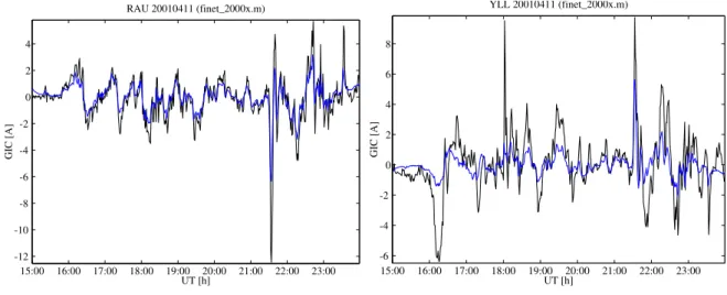
The conductivity model of Table 2 is quite reasonable for southern Finland. For Rauma, the fit is good, and us-ing slightly smaller conductivities further improves the re-sult due to an increased electric field. Concerning Yllikk¨al¨a, clearly smaller values of the conductivity would seem neces-sary. However, the lack of good data from Yllikk¨al¨a prevents a detailed analysis.

To show that a modified conductivity model improves model results, we considered 10 stormy days in 1999–2001 (Table 3). There is a high correlation between the measured

A. Viljanen et al.: Fast computation of the geoelectric field 107 16:000 17:00 18:00 19:00 20:00 21:00 20 40 60 80 100 120 140 160 180 200 220 UT [h] sum(GIC) [A] 20010411 01:300 02:00 02:30 03:00 03:30 04:00 04:30 05:00 50 100 150 200 250 UT [h] sum(GIC) [A] 20011106

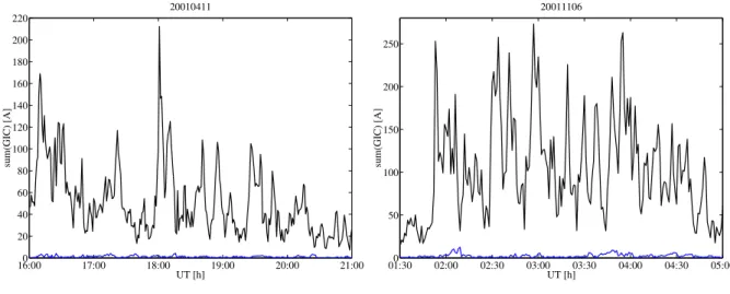
Fig. 6. Comparison of the sum of the absolute values of geomagnetically induced currents in the nodes

of the Finnish high-voltage power system (April 11, 2001 and November 6, 2001), as calculated with

the complex image method (black line) and the local 1D method. The absolute value of the difference is

plotted as a blue line. In both cases, the total horizontal magnetic variation field is the same. The earth’s

conductivity model is given in Table 2.

max = 55 mV/km

21:30:00

max = 162 mV/km

21:31:00

max = 431 mV/km

21:32:00

max = 436 mV/km

21:33:00

max = 365 mV/km

21:34:00

max = 247 mV/km

21:35:00

max = 169 mV/km

21:36:00

max = 156 mV/km

21:37:00

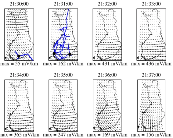
Fig. 7. Snapshots of the calculated electric field on April 11, 2001, using the local 1D method and the

earth model of Table 2. The main parts of the Finnish natural gas pipeline are sketched in the first plot

with blue lines and the measuring site at M¨ants¨al¨a is marked as a black dot. The Finnish 400 kV and

220 kV power lines are shown in the second plot with blue lines. The Rauma and Yllikk¨al¨a 400 kV

transformers are the black dots in the west and east, respectively.

28

Fig. 6. Comparison of the sum of the absolute values of geomagnetically induced currents in the nodes of the Finnish high-voltage power

system (11 April 2001 and 6 November 2001), as calculated with the complex image method (black line) and the local 1-D method. The absolute value of the difference is plotted as a blue line. In both cases, the total horizontal magnetic variation field is the same. The Earth’s conductivity model is given in Table 2.

Table 2. A simple Earth conductivity model used in this study

(Vil-janen et al., 1999b) depth [km] resistivity [m] 0 - 3 5000 3 - 9 500 9 - 14 100 14 - 21 10 21 - 44 20 44 - 150 1000 150 - 1

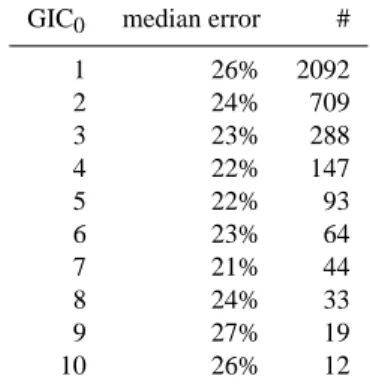
and modelled values during all events. A linear regression analysis shows that multiplying measured values by 1.8844 yields the best fit when GIC larger than 1 A is considered. A rough way to modify the Earth model is to divide the conduc-tivities of each layer by 1.88442 ≈ 3.55. This would work exactly with a uniform Earth, since then the electric field is inversely proportional to the square root of the conductivity. With this simple division of all conductivities of the layered model, we obtain the model errors given in Table 4. The measuring noise is at least ±0.5 A, so the fit is quite reason-able. A more systematic procedure would be necessary for an objective way to modify the Earth model. A division of conductivities by a constant does not necessarily yield the optimal result, but it is obviously necessary to change layer thickness, too.

Taking into account that Rauma is located close to the southern boundary of IMAGE and that the nearest magnetic station Nurmij¨arvi is at a distance of 200 km, the correspon-dence between the modelled shape of the GIC curve is good. This is not completely surprising, because the electric field in Fig. 7 varies quite smoothly in a length scale of 100–200 km

Table 3. Stormy events used in the comparison of measured and

modelled GIC at Rauma. The second column gives the linear cor-relation coefficient between the measured and modelled values.

day correlation 19990922 0.839 20000406 0.723 20000715 0.922 20000917 0.840 20001106 0.901 20010331 0.925 20010411 0.914 20011106 0.896 20020907 0.860 20021001 0.884

in southern Finland. This is in concert with the results by Vil-janen et al. (2001), who found that large dH/dt vectors tend to be north-south oriented in the subauroral region, whereas in the auroral region there is no clear preference of direction. So at subauroral latitudes, there is evidently less spatial vari-ations in ionospheric currents than at higher latitudes. 3.2.2 Finnish natural gas pipeline

Calculation of GIC in a pipeline is basically similar to the power system. Two examples in Fig. 9 show that the shape of the modelled curve again follows closely the measured one. This is expected, since the pipeline is located in the same region as the southern part of the power system, and GIC model results are good for it (Fig. 8). Correlation coefficients between the modelled and measured values are mostly larger than 0.8. As discussed by Pulkkinen et al. (2001b), the active cathodic protection system tries to keep the pipe-to-soil

volt-108 A. Viljanen et al.: Fast computation of the geoelectric field 16:000 17:00 18:00 19:00 20:00 21:00 20 40 60 80 100 120 140 160 180 200 220 UT [h] sum(GIC) [A] 20010411 01:300 02:00 02:30 03:00 03:30 04:00 04:30 05:00 50 100 150 200 250 UT [h] sum(GIC) [A] 20011106

Fig. 6. Comparison of the sum of the absolute values of geomagnetically induced currents in the nodes

of the Finnish high-voltage power system (April 11, 2001 and November 6, 2001), as calculated with

the complex image method (black line) and the local 1D method. The absolute value of the difference is

plotted as a blue line. In both cases, the total horizontal magnetic variation field is the same. The earth’s

conductivity model is given in Table 2.

max = 55 mV/km

21:30:00

max = 162 mV/km

21:31:00

max = 431 mV/km

21:32:00

max = 436 mV/km

21:33:00

max = 365 mV/km

21:34:00

max = 247 mV/km

21:35:00

max = 169 mV/km

21:36:00

max = 156 mV/km

21:37:00

Fig. 7. Snapshots of the calculated electric field on April 11, 2001, using the local 1D method and the

earth model of Table 2. The main parts of the Finnish natural gas pipeline are sketched in the first plot

with blue lines and the measuring site at M¨ants¨al¨a is marked as a black dot. The Finnish 400 kV and

220 kV power lines are shown in the second plot with blue lines. The Rauma and Yllikk¨al¨a 400 kV

transformers are the black dots in the west and east, respectively.

28

Fig. 7. Snapshots of the calculated electric field on 11 April 2001, using the local 1-D method and the Earth model of Table 2. The main

parts of the Finnish natural gas pipeline are sketched in the first plot with blue lines, and the measuring site at M¨ants¨al¨a is marked as a black dot. The Finnish 400 kV and 220 kV power lines are shown in the second plot with blue lines. The Rauma and Yllikk¨al¨a 400 kV transformers are the black dots in the west and east, respectively.

age constant, so it tends to decrease GIC. The conductivity model happens to be quite suitable, implicitly correcting this bias, too.

3.2.3 Plane wave model

In the previous examples, the geoelectric field was calculated using a spatially nonuniform magnetic field. Then the elec-tric field also varies spatially at each time step. It follows that, for example, voltages between nodes in a power system must be integrated separately at each instant. On the other hand, if we can assume that the electric field does not vary spatially then GIC at each time step is

GI C(t ) = aEx(t ) + bEy(t ) (4)

where a and b depend on the topology and resistances of the network. This method was used, for example, by Viljanen and Pirjola (1989), who calculated GIC in the Finnish power system using magnetic data of the Nurmij¨arvi observatory. It turned out that GIC at a site of about 300 km northeast from the observatory could not be modelled very well. The ob-vious explanation was that magnetic field variations around the GIC site are usually not sufficiently similar to that at Nur-mij¨arvi.

However, the plane wave method is useful if the electric field is calculated so that the magnetic field is the field ob-served or interpolated at the GIC site of interest. This means that for each GIC site we select an Earth model used globally. This is slightly different from the local 1-D method discussed above, in which we can use a different model for each Earth surface grid point. The benefit of the plane wave model is that GIC is obtained simply by Eq. (4). Next, we will demon-strate that the plane wave method is really applicable. We use all available GIC data of April, September–November 2001, and also of the other events listed in Table 3.

With the plane wave assumption, GIC at M¨ants¨al¨a is

GI C(A) = −70Ex+88Ey, where the electric field is given

in V/km (Pulkkinen et al., 2001b). We now assume that the Earth is uniform. Since we are interested in large currents, we considered only (absolute) values larger than 1 A when searching for the optimal value of the conductivity. Results are given in Tables 5–6. The conductivity value depends on the way the linear fit is made: the larger value is obtained when we express the measured values as a function of the modelled ones. The smaller value is obtained when we make the fit vice versa. The smaller conductivity yields a better fit for small currents, but for the largest currents the larger con-ductivity is a better choice. A slightly better fit for large

cur-A. Viljanen et al.: Fast computation of the geoelectric field 109

Table 4. Misfit of modelled GIC values at Rauma during the events

used in Table 3. The first column gives the lower limit of (absolute) GIC values considered. The second column gives the median error of modelled values. The last column gives the number of measured one-minute values larger than GI C0. The Earth model is explained

in the text

GIC0 median error #

1 26% 2092 2 24% 709 3 23% 288 4 22% 147 5 22% 93 6 23% 64 7 21% 44 8 24% 33 9 27% 19 10 26% 12

rents was found with a conductivity 0.050 ohmm−1. So this value could be a reasonable choice for M¨ants¨al¨a. Pulkkinen et al. (2001b) used the value 0.031 ohmm−1based on a sam-ple event. Using a properly constructed multi-layer model would evidently provide the best fit, but finding such a model is non-trivial.

GIC at Rauma in the plane wave model is GI C(A) =

−1.9Ex −22.3Ey, where the electric field is expressed in

V/km. Now GIC depends practically only on Ey, which in

turn is determined by dX/dt. We used the interpolated mag-netic field at Rauma (Table 7) or directly the field measured at Nurmij¨arvi (Table 8). The use of the Nurmij¨arvi field pro-vides nearly equally good results. There are two reasons for this: Rauma and Nurmij¨arvi are at about the same latitude, and latitudinal dX/dt variations in the subauroral region are not very strong (Viljanen et al., 2001), cf. also Fig. 7. Nur-mij¨arvi is also the closest magnetometer station to Rauma, so it has the largest effect on the interpolated field. We tested this hypotheses by calculating GIC using the measured mag-netic field at Hankasalmi (62.30 N, 26.65 E) about 250 km northeast from Rauma (Table 9). Now the errors are clearly larger, indicating that the time derivative of the magnetic field varies more in the north-south direction than in the east-west direction, at least in the subauroral region.

3.2.4 Computational performance

We present here some illustrative numbers of computation times of the full determination of GIC in the Finnish power system. We used a 867 MHz laptop and MatLab by vectoris-ing the code as much as possible, but without usvectoris-ing external compiled subroutines. In the following, we consider a one-day event of 1440 one-minute values.

1. Calculation of the ionospheric equivalent currents using the measured ground magnetic field. The number of

Table 5. Misfit of modelled GIC values at M¨ants¨al¨a during April,

September-November 2001, and during the other events listed in Ta-ble 3. The first column gives the lower limit of (absolute) GIC val-ues considered. The second column gives the median error of mod-elled values. The last column shows the number of measured 10-s values larger than GI C0. The electric field was calculated using

only the magnetic data of the Nurmij¨arvi observatory. A uniform Earth model was assumed with a conductivity of 0.07663 ohmm−1.

GIC0 median error #

2 38% 17106 4 34% 5580 6 33% 2357 8 29% 1157 10 27% 650 12 26% 357 14 22% 226 16 23% 152 18 22% 93 20 20% 61 22 20% 35 24 24% 22

ionospheric grid points was about 400. Calculation of currents takes about 3 s.

2. Interpolation of the magnetic field at the Earth’s surface (three components). Using 231 points to cover Finland takes about 13 s per day. However, a smaller number of points (around 60) is needed if the plane wave method is used for each power system node separately.

3. Calculation of the electric field at the Earth grid points. With FFT this takes 25 s for 231 points. (We do not force the time series to be of length 2n for an optimal FFT.) Again, the plane wave method would reduce the time due to a smaller number of grid points.

4. Calculation of GIC in the power system nodes and trans-mission lines. If the electric field varies spatially, then it must be integrated separately for each time step, which takes 137 s for 62 nodes and 68 lines. The slowness of this phase is mainly due to the need to interpolate the electric field for a numerical integration along transmis-sion lines. However, if the plane wave method is used then GIC is obtained from Eq. (4), which takes a small amount of time.

Altogether, with the local 1-D method, it takes about 3 min to execute the computation for the Finnish power system for a one-day event using one-minute values. With the plane wave method, it takes less than half a minute. In any case, the computation time is fast enough for an extensive event post analysis.

An operational application is the real-time calculation of GIC in the Finnish natural gas pipeline system within the European Space Agency Space Weather Pilot Programme

110 A. Viljanen et al.: Fast computation of the geoelectric field 15:00 16:00 17:00 18:00 19:00 20:00 21:00 22:00 23:00 -12 -10 -8 -6 -4 -2 0 2 4 UT [h] GIC [A] RAU 20010411 (finet_2000x.m) 15:00 16:00 17:00 18:00 19:00 20:00 21:00 22:00 23:00 -6 -4 -2 0 2 4 6 8 UT [h] GIC [A] YLL 20010411 (finet_2000x.m)

Fig. 8. Measured (black line) and modelled (blue line) geomagnetically induced currents at the Rauma

(RAU) and Yllikk¨al¨a (YLL) 400 kV transformer stations on April 11, 2001.

19:00 20:00 21:00 22:00 23:00 -15 -10 -5 0 5 10 15 20 25 30 35 UT [h] GIC [A] 20000715 15:00 16:00 17:00 18:00 19:00 20:00 21:00 -15 -10 -5 0 5 10 15 UT [h] GIC [A] 20010331

Fig. 9. Measured (black line) and modelled (blue line) geomagnetically induced currents along the

Finnish natural gas pipeline at M¨ants¨al¨a on July 15, 2000 and on March 31, 2001. The geoelectric field

is calculated by the complex image method.

29

Fig. 8. Measured (black line) and modelled (blue line) geomagnetically induced currents at the Rauma (RAU) and Yllikk¨al¨a (YLL) 400 kV

transformer stations on 11 April 2001.

15:00 16:00 17:00 18:00 19:00 20:00 21:00 22:00 23:00 -12 -10 -8 -6 -4 -2 0 2 4 UT [h] GIC [A] RAU 20010411 (finet_2000x.m) 15:00 16:00 17:00 18:00 19:00 20:00 21:00 22:00 23:00 -6 -4 -2 0 2 4 6 8 UT [h] GIC [A] YLL 20010411 (finet_2000x.m)

Fig. 8. Measured (black line) and modelled (blue line) geomagnetically induced currents at the Rauma

(RAU) and Yllikk¨al¨a (YLL) 400 kV transformer stations on April 11, 2001.

19:00 20:00 21:00 22:00 23:00 -15 -10 -5 0 5 10 15 20 25 30 35 UT [h] GIC [A] 20000715 15:00 16:00 17:00 18:00 19:00 20:00 21:00 -15 -10 -5 0 5 10 15 UT [h] GIC [A] 20010331

Fig. 9. Measured (black line) and modelled (blue line) geomagnetically induced currents along the

Finnish natural gas pipeline at M¨ants¨al¨a on July 15, 2000 and on March 31, 2001. The geoelectric field

is calculated by the complex image method.

29

Fig. 9. Measured (black line) and modelled (blue line) geomagnetically induced currents along the Finnish natural gas pipeline at M¨ants¨al¨a

on 15 July 2000 and on 31 March 2001. The geoelectric field is calculated by the complex image method.

started in spring 2003. The magnetic field data is retrieved from Nurmij¨arvi and the electric field is calculated assum-ing that the field does not vary over the pipeline system. As shown in this paper, a fairly good prediction is then expected for GIC. The pipeline company can use the nowcasted GIC as additional information to distinguish between geomagnetic and other reasons for disturbances in the corrosion protec-tion system. Because the magnetic field is used only from one site, the electric field is obtained practically immediately. The same is true for GIC determined with Eq. (4).

4 Conclusions

A powerful method to calculate the geoelectric field for space weather purposes is presented in this paper. It needs only two inputs: the horizontal geomagnetic variation field at the

Earth’s surface, and 1-D models of the Earth’s conductivity. The method of spherical elementary current systems (SECS) allows for interpolating the magnetic field at any ground point. Assuming a planar geometry, the geoelectric field is obtained by the surface impedance relation from the local magnetic field using a local 1-D model of the Earth’s con-ductivity. The validity of the local 1-D method was proved by comparisons of measured and modelled electric fields and geomagnetically induced currents (GIC). Especially con-cerning GIC, spatially averaged electric fields are obtained with a good accuracy.

A handy way is to consider each GIC site separately, as-suming that the magnetic field does not vary spatially, which is the plane wave model. Then GIC is obtained by a multi-plication of the horizontal electric field components by con-stants, which are determined by resistances and the geometry

A. Viljanen et al.: Fast computation of the geoelectric field 111

Table 6. As Table 5, but with a conductivity of 0.03993 ohmm−1.

GIC0 median error #

2 36% 17106 4 33% 5580 6 32% 2357 8 32% 1157 10 31% 650 12 30% 357 14 29% 226 16 28% 152 18 27% 93 20 27% 61 22 25% 35 24 20% 22

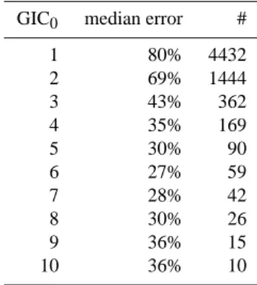
Table 7. Misfit of modelled GIC values at Rauma during the events

listed in Table 3. The first column gives the lower limit of (abso-lute) GIC values considered. The second column gives the median error of modelled values. The last column shows the number of measured one-minute values larger than GI C0. Interpolated values

of the magnetic field at Rauma were used to calculate the electric field. The conductivity of the uniform Earth was 0.01309 ohmm−1.

GIC0 median error #

1 76% 4432 2 65% 1444 3 43% 362 4 28% 169 5 23% 90 6 23% 59 7 22% 42 8 22% 26 9 23% 15 10 23% 10

of the technological conductor system. So this is a some-what simpler way than that used by Pulkkinen et al. (2000) and Erinmez et al. (2002), in which the electric field must be integrated along conductors separately for each time step. Although the plane wave model neglects the spatial variation of the magnetic field, it provides a good prediction for the electric field in a sufficiently large region around the site un-der study. In other words, the voltages induced in conductors near the specific site have the largest contribution to GIC at that site. The key point is that the magnetic field must be accurately determined at the GIC site. Some earlier attempts like Viljanen and Pirjola (1989) partly failed due to using the magnetic field measured at a distant location. Now the inter-polation of the field by the SECS method fixes this problem. Dense magnetometer arrays are typically located in sparsely-populated areas in the auroral region. The Finnish natural gas pipeline and most of the high-voltage power sys-tem lie in the subauroral area, where there are only some

Table 8. As Table 7, but the magnetic field at Nurmij¨arvi was used

to calculate the electric field.

GIC0 median error #

1 77% 4432 2 64% 1444 3 43% 362 4 32% 169 5 26% 90 6 28% 59 7 24% 42 8 26% 26 9 28% 15 10 25% 10

Table 9. As Table 8, but the magnetic field at Hankasalmi was used

to calculate the electric field.

GIC0 median error #

1 80% 4432 2 69% 1444 3 43% 362 4 35% 169 5 30% 90 6 27% 59 7 28% 42 8 30% 26 9 36% 15 10 36% 10

magnetic observation sites. It follows that the spatial accu-racy of ionospheric equivalent currents is inevitably smaller than in the auroral region. This is not necessarily a limitation to the usefulness of the calculation method of the electric field, provided that relevant spatial scales are of the same or-der as magnetometer separations. There is some indication that large subauroral GIC events are more often related to large-scale electrojets than at high latitudes (Viljanen et al., 2001), but further studies are necessary (e.g. Pulkkinen et al., 2003c). From the practical viewpoint, most of the systems vulnerable to GIC are located farther south than the Finnish power grid. So the local 1-D method validated in the subau-roral region evidently works well also in mid-latitudes with spatially smoother magnetic fields.

In the future, it may be possible to include detailed 3-D models of the Earth, and perform calculations of the electric field with the multisheet modelling technique, as, for exam-ple, by Engels et al. (2002). However, much more compu-tational power is required before such an approach will be feasible for studying large sets of events.

The next step would be using the local 1-D and plane wave methods in GIC forecasting (cf. Kappenman et al., 2000; Erinmez et al., 2002). The ultimate goal in space weather

112 A. Viljanen et al.: Fast computation of the geoelectric field research is to provide forecasts in the same way as normal

weather forecasts are given today. Concerning the geoelec-tric field, the ground magnetic variation field should be pre-dicted. Today’s skills are not yet good enough for really ac-curate forecasting, but there are rapidly developing efforts to improve this in the way required in GIC forecasting (Gleis-ner and Lundstedt, 2001; Valdivia et al., 1999; Weigel et al., 2002).

The method described in this paper is also applicable to magnetotelluric studies. Its first step includes an equivalent description of ionospheric currents, so it gives full control on the source field. Second, Earth models can be directly tested with the local 1-D method for any events. GIC are related to a spatially smoothed electric field, so they yield information on Earth’s conductivity in a regional scale, and the 1-D assumption seems then reasonable, as in the southern Finland area considered in this paper.

Acknowledgement. The Academy of Finland supported the works

of O.A. and A.P. We thank all institutes maintaining the IMAGE magnetometer network. INTAS funded partly the BEAR project (no. 97-1162). Fingrid Oyj and Gasum Oy are acknowledged for a fruitful co-operation on geomagnetically induced currents in the Finnish high-voltage power system and in the Finnish natural gas pipeline, respectively.

The Editor in Chief thanks I. Ferguson and another referee for their help in evaluating this paper.

References

Amm, O.: Ionospheric Elementary Current Systems in Spherical Coordinates and Their Application, J. Geomag. Geoelectr., 49, 947–955, 1997.

Amm, O. and Viljanen, A.: Ionospheric disturbance magnetic field continuation from the ground to the ionosphere using spherical elementary current systems, Earth Planets Space, 51, 431–440, 1999.

Bolduc, L.: GIC observations and studies in the Hydro-Quebec power system, J. Atmos. Sol.-Terr. Phys., 64, 1793–1802, 2002. Boteler, D. H. and Pirjola, R. J.: The complex-image method for

calculating the magnetic and electric fields produced at the sur-face of the Earth by the auroral electrojet, Geophys. J. Int., 132, 31–40, 1998.

Boteler, D. H., Pirjola, R. J.,and Nevanlinna, H.: The effects of ge-omagnetic disturbances on electrical systems at the Earth’s sur-face, Adv. Space Res., 22, 17–27, 1998.

Dmitriev, V. and Berdichevsky, M.: The fundamental model of magnetotelluric sounding, IEEE Proc., 67, 1034, 1979.

Engels, M., Korja, T., and the BEAR Working Group: Multi-sheet modelling of the electrical conductivity structure in the Fennoscandian Shield, Earth Planets Space, 54, 559–573, 2002. Erinmez, I. A., Kappenman, J. G., and Radasky, W. A.:

Manage-ment of the geomagnetically induced current risks on the national grid company’s electric power transmission system, J. Atmos. Sol.-Terr. Phys., 64, 743–756, 2002.

Gleisner, H. and Lundstedt, H.: A neural network-based local model for prediction of geomagnetic disturbances, J. Geophys. Res., 106, 8425–8433, 2001.

Gummow, R. A.: GIC effects on pipeline corrosion control systems, J. Atmos. Sol.-Terr. Phys., 64, 1755–1764, 2002.

Kappenman, J. G.: Geomagnetic Storms and Their Impact on Power Systems, IEEE Power Engineering Review, May 1996, 5–8, 1996.

Kappenman, J. G., Radasky, W. A., Gilbert, J. L., and Erinmez, I. A.: Advanced Geomagnetic Storm Forecasting: A Risk Man-agement Tool for Electric Power System Operations, IEEE T. Plasma Sci., 28, 2114–2121, 2000.

Korja, T., Engels, M., Zhamaletdinov, A. A., Kovtun, A. A., Pal-shin, N. A., Smirnov, M. Yu., Tokarev, A. D., Asming, V. E., Vanyan, L. L., Vardaniants, I. L., and the BEAR Working Group: Crustal conductivity in Fennoscandia – a compilation of a database on crustal conductance in the Fennoscandian Shield, Earth Planets Space, 54, 535–558, 2002.

Lahtinen, M. and Elovaara, J.: GIC Occurrences and GIC Test for 400 kV System Transformer, IEEE T. Power Delivery, 17, 555– 561, 2002.

Lehtinen, M. and Pirjola, R.: Currents produced in earthed conduc-tor networks by geomagnetically-induced electric fields, Ann. Geophysicae, 3, 479–484, 1985.

Lesher, R. L., Porter, J. W., and Byerly, R. T.: SUNBURST – A Network of GIC Monitoring Systems, IEEE T. Power Deliver., 9, 128–137, 1994.

Lindell, I. V., H¨anninen, J. J., and Pirjola, R.: Wait’s Complex-Image Principle Generalized to Arbitrary Sources, IEEE T. An-tennas Propagat., 48, 1618–1624, 2000.

Mareschal, M.: Modelling of natural sources of magnetospheric ori-gin in the interpretation of regional induction studies: a review, Surv. Geophys., 8, 261–300, 1986.

Molinski, T. S.: Why utilities respect geomagnetically induced cur-rents, J. Atmos. Sol.-Terr. Phys., 64, 1765–1778, 2002.

Osella, A., Favetto, A., and Lopez, E.: Currents induced by geo-magnetic storms on buried pipelines as a cause of corrosion, J. Appl. Geophys., 38, 219–233, 1998.

Osipova, I. L., Hjelt, S. E., and Vanyan, L. L.: Source field problems in northern parts of the Baltic Shield, Phys. Earth Planet. Int., 53, 337–342, 1989.

Pirjola, R. and Viljanen, A.: Complex image method for calculating electric and magnetic fields produced by an auroral electrojet of a finite length, Ann. Geophysicae, 16, 1434–1444, 1998. Pirjola, R., Pulkkinen, A., and Viljanen, A.: Studies of Space

Weather Effects on the Finnish Natural Gas Pipeline and on the Finnish High-Voltage Power System, accepted for publication in Adv. Space Res., 2002.

Pulkkinen, A., Viljanen, A., Pirjola, R., and BEAR Working Group: Large geomagnetically induced currents in the Finnish high-voltage power system, Finn. Meteorol. Inst. Rep., 2000:2, 99 pp., 2000.

Pulkkinen, A., Pirjola, R., Boteler, D., Viljanen, A., and Yegorov, I.: Modelling of space weather effects on pipelines, J. Appl. Geo-phys., 48, 233–256, 2001a.

Pulkkinen, A., Viljanen, A., Pajunp¨a¨a, K., and Pirjola, R.: Record-ings and occurrence of geomagnetically induced currents in the Finnish natural gas pipeline network, J. Appl. Geophys., 48, 219–231, 2001b.

Pulkkinen, A., Amm, O., Viljanen, A., and BEAR Working Group: Ionospheric equivalent current distributions determined with the method of spherical elementary current systems, J. Geophys. Res., 108(A2), 1053, doi:10.1029/2001JA005085, 2003a. Pulkkinen, A., Amm, O., Viljanen, A., and BEAR Working Group:

Separation of the geomagnetic variation field into external and internal parts using the spherical elementary current system method, Earth Planets Space, 55, 117–129, 2003b.

A. Viljanen et al.: Fast computation of the geoelectric field 113

Pulkkinen, A., Thomson, A., Clarke, E., and McKay, A.: April 2000 storm: ionospheric drivers of large geomagnetically induced cur-rents, Ann. Geophysicae, 21, 709–717, 2003c.

Tanskanen, E. I., Viljanen, A., Pulkkinen, T. I., Pirjola, R., H¨akkinen, L., Pulkkinen, A., and Amm, O.: At substorm on-set, 40% of AL comes from underground, J. Geophys. Res., 106, 13 119–13 134, 2001.

Thomson, D. J., and Weaver, J. T.: The Complex Image Approxi-mation for Induction in a Multilayered Earth, J. Geophys. Res., 80, 123–129, 1975.

Trichtchenko, L. and Boteler, D. H.: Modelling of geomagnetic in-duction in pipelines, Ann. Geophysicae, 20, 1063–1072, 2002. Valdivia, J. A., Vassiliadis, D., Klimas, A., and Sharma, A. S.:

Mod-eling the spatial structure of the high latitude magnetic pertur-bations and the related current systems, Physics of Plasmas, 6, 4185–4194, 1999.

Viljanen, A. and Pirjola, R.: Statistics on geomagnetically-induced currents in the Finnish 400 kV power system based on recordings of geomagnetic variations. J.Geomagnetism and Geoelectricity,

41, 411–420, 1989.

Viljanen, A., Amm, O., and Pirjola, R.: Modelling Geomagneti-cally Induced Currents During Different Ionospheric Situations, J. Geophys. Res., 104, 28 059–28 072, 1999a.

Viljanen, A., Pirjola, R., and Amm, O.: Magnetotelluric source effect due to 3-D ionospheric current systems using the com-plex image method for 1-D conductivity structures, Earth Planets Space, 51, 933–945, 1999b.

Viljanen, A., Nevanlinna, H., Pajunp¨a¨a, K., and Pulkkinen, A.: Time derivative of the horizontal geomagnetic field as an activity indicator, Ann. Geophysicae, 19, 1107–1118, 2001.

Wait, J. R. and Spies, K. P.: On the image representation of the quasi-static fields of a line current source above the ground, Can. J. Phys., 47, 2731–2733, 1969.

Weigel, R. S., Vassiliadis, D., and Klimas, A. J.: Coupling of the solar wind to temporal fluctuations in ground magnetic fields, Geophys. Res. Lett., 29, No. 19, doi:10.1029/2002GL014740, 2002.