Climatological lower thermosphere winds as seen by ground-based and space-based instruments

(1)

HAL Id: hal-00317393

https://hal.archives-ouvertes.fr/hal-00317393

Submitted on 14 Jun 2004

HAL is a multi-disciplinary open access

archive for the deposit and dissemination of

sci-entific research documents, whether they are

pub-lished or not. The documents may come from

teaching and research institutions in France or

abroad, or from public or private research centers.

L’archive ouverte pluridisciplinaire HAL, est

destinée au dépôt et à la diffusion de documents

scientifiques de niveau recherche, publiés ou non,

émanant des établissements d’enseignement et de

recherche français ou étrangers, des laboratoires

publics ou privés.

ground-based and space-based instruments

J. M. Forbes, Yu. I. Portnyagin, W. Skinner, R. A. Vincent, T. Solovjova, E.

Merzlyakov, T. Nakamura, S. Palo

To cite this version:

J. M. Forbes, Yu. I. Portnyagin, W. Skinner, R. A. Vincent, T. Solovjova, et al.. Climatological lower

thermosphere winds as seen by ground-based and space-based instruments. Annales Geophysicae,

European Geosciences Union, 2004, 22 (6), pp.1931-1945. �hal-00317393�

(2)

SRef-ID: 1432-0576/ag/2004-22-1931 © European Geosciences Union 2004

Annales

Geophysicae

Climatological lower thermosphere winds as seen by ground-based

and space-based instruments

J. M. Forbes1, Yu. I. Portnyagin2, W. Skinner3, R. A. Vincent4, T. Solovjova2, E. Merzlyakov2, T. Nakamura5, and S. Palo1

1_{Department of Aerospace Engineering Sciences, University of Colorado, Boulder, CO 80309, USA}

2_{Institute for Experimental Meteorology, SPA Typhoon, Obninsk, Russia}

3_{Space Physics Research Laboratory, University of Michigan, Ann Arbor, MI, USA}

4_{Department of Physics and Mathematical Physics, University of Adelaide, Adelaide 5005 SA, Australia} 5_{Radio Atmospheric Science Center, Kyoto University, Kyoto, Japan}

Received: 30 January 2003 – Revised: 9 February 2004 – Accepted: 25 February 2004 – Published: 14 June 2004

Abstract. Comparisons are made between climatological

dynamic fields obtained from ground-based (GB) and space-based (SB) instruments with a view towards identifying SB/GB intercalibration issues for TIMED and other future aeronomy satellite missions. SB measurements are made from the High Resolution Doppler Imager (HRDI) instru-ment on the Upper Atmosphere Research Satellite (UARS). The GB data originate from meteor radars at Obninsk, (55◦N, 37◦E), Shigaraki (35◦N, 136◦E) and Jakarta (6◦S,

107◦E) and MF spaced-antenna radars at Hawaii (22◦N,

160◦W), Christmas I. (2◦N, 158◦W) and Adelaide (35◦S, 138◦E). We focus on monthly-mean prevailing, diurnal and semidiurnal wind components at 96 km, averaged over the 1991–1999 period. We perform space-based (SB) analyses for 90◦_{longitude sectors including the GB sites, as well as} for the zonal mean. Taking the monthly prevailing zonal winds from these stations as a whole, on average, SB zonal winds exceed GB determinations by ∼63%, whereas merid-ional winds are in much better agreement. The origin of this discrepancy remains unknown, and should receive high pri-ority in initial GB/SB comparisons during the TIMED mis-sion.

We perform detailed comparisons between monthly clima-tologies from Jakarta and the geographically conjugate sites of Shigaraki and Adelaide, including some analyses of in-terannual variations. SB prevailing, diurnal and semidiur-nal tides exceed those measured over Jakarta by factors, on the average, of the order of 2.0, 1.6, 1.3, respectively, for the eastward wind, although much variability exists. For the meridional component, SB/GB ratios for the diurnal and semidiurnal tide are about 1.6 and 1.7. Prevailing and tidal amplitudes at Adelaide are significantly lower than SB

val-Correspondence to: J. M. Forbes

(forbes@colorado.edu)

ues, whereas similar net differences do not occur at the con-jugate Northern Hemisphere location of Shigaraki. Adelaide diurnal phases lag SB phases by several hours, but excellent agreement between the two data sources exists for semidiur-nal tidal phases throughout the year. These results are con-sistent with phase retardation effects in the MF radar tech-nique that are thought to exist above about 90 km. Prevail-ing and tidal amplitudes from Shigaraki track year-to-year variations in SB fields, whereas in the Southern Hemisphere poorer agreement exists. The above hemispheric differences are due in part to MF vs. meteor radar techniques, but zonal asymmetries and day-to-day variability, combined with inad-equate sampling, may also be playing a role. Based on these results, some obvious recommendations emerge that are rele-vant to combined GB/SB studies as part of TIMED and other future aeronomy missions.

Key words. Meteorology and atmospheric dynamics

(ther-mospheric dynamics; waves and tides; instruments and tech-niques)

1 Introduction

The dynamics of the mesosphere and lower thermosphere (MLT, ca. 80–150 km) contains large contributions from gravity waves, thermal tides, and planetary-scale waves that originate in the lower atmosphere, grow exponentially with height, and dissipate in this region. Winds in this region are measured from the ground (i.e. by various radar and opti-cal methods) and from space (i.e. by optiopti-cal interferome-try). Ground-based (GB) instruments have the obvious ad-vantage of good time resolution, but are distributed sparsely over the globe. Space-based (SB) measurements offer global

(3)

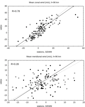
Mean zonal wind (m/s), h=96 km stations, GEWM HRDI -40 -20 0 20 40 60 80 -40 -20 0 20 40 60 R=0.78

Mean meridional wind (m/s), h=96 km

stations, GEWM HRDI -20 -15 -10 -5 0 5 10 15 20 -20 -15 -10 -5 0 5 10 15 20 R=0.28

Fig. 1. Scatter plots of HRDI monthly mean zonal winds at latitudes 52◦N, 35◦N, 22◦N, 2◦N, 6◦S, and 35◦S, representing averages of measurements made during the 1991–1999 period, versus the corresponding ground-based measurements at the same latitudes. Filled circles: HRDI winds versus winds measured at the individual MF and meteor radar stations (Obninsk, 52◦N; Shigaraki, 35◦N; Hawaii, 22◦N (1991–1992); Christmas I., 2◦N; Jakarta, 6◦S; Ade-laide, 35◦S); the solid line is the corresponding least-squares fit. Open circles: HRDI winds versus the corresponding GEWM winds at the same latitudes; least-squares fit to these data is the broken line. Top: zonal winds. Bottom: meridional winds. All data are at a height of 96 km.

coverage, but poor time resolution at various points fixed on the Earth. In order to deconvolve unambiguously the spa-tial and temporal characteristics of the dynamically evolving MLT circulation, it is becoming increasingly evident that the SB and GB measurements need to be assimilated together in some way. This requires the SB and GB measurements to consistently represent the dynamical circulation, or that they be intercalibrated so that consistency is achieved. Develop-ment and application of GB/SB assimilation techniques are likely to assume important roles in achieving the scientific objectives of the NASA TIMED (Thermosphere-Ionosphere-Mesosphere Energetics and Dynamics) mission that was ini-tiated by launch of the TIMED satellite on 7 December 2001. The purpose of this paper is to present comparisons be-tween climatological GB and SB wind measurements repre-sentative of the UARS (Upper Atmosphere Research Satel-lite) mission during 1991–1999, and to identify the inter-calibration issues that emerge from this effort. This

infor-mation is anticipated to be of significant value to similar activities likely to emerge within TIMED and other future missions. The data utilized here are from the High Res-olution Doppler Imager (HRDI) instrument on UARS, and from several radars and a global empirical model. Previ-ous SB/GB wind comparisons using UARS data (see, for example, Burrage et al., 1996) have primarily concentrated on statistical analyses of accumulated “overflight” or “co-incident” measurements. The pitfalls of overflight compar-isons are well known. “Coincidence” is considered to ex-ist out to a radial dex-istance of ∼1000 km. The SB measure-ment is nearly instantaneous, but represents an average ve-locity over ∼500 km along the line of sight. In contrast, the radar measurement is spatially local, but may be aver-aged over ∼1 h prior to comparison with the SB data. On the other hand, it is well accepted and intuitively clear that high spatial coherence exists in multi-year average fields for the lowest-frequency components of the atmospheric circulation (i.e. prevailing winds, diurnal and semidiurnal tides, month-to-month and interannual variations). In this case, the pre-viously mentioned difficulties of overflight comparisons are reduced considerably. The focus of this paper is to conduct such a climatological comparison.

A similar but more limited study involving winds from the Wind-Imaging Interferometer (WINDII) instrument on UARS was conducted by Portnyagin et al. (1999). They uti-lized the GEWM (Global Empirical Wind Model; Portnya-gin and Solovjova, 2000) as being representative of the cli-matology of mesosphere and lower thermosphere dynamics as seen by ground-based radars. Their study was restricted to the zonal mean wind field. They found a degree of con-sistency between climatologies representative of GB and SB data sources, in that the annual and semiannual components of the zonal mean wind field were very similar. However, a systematic bias was found between the annual mean zonal winds, with the GEWM winds being generally smaller than those of WINDII by a factor of 2.0–2.5. This bias is practi-cally independent of altitude and can be described by a term of Acos4θ , where A is about 20 ms−1and θ is colatitude.

The following section describes the data utilized in the study. Section 3 presents our results, and Sect. 4 summa-rizes our conclusions and identifies issues that need to be ad-dressed in connection with SB/GB comparisons anticipated for the NASA TIMED mission.

In this paper we utilize the following abbreviations: GB (ground-based); SB (space-based); u (zonal, or eastward wind component); v (meridional or northward wind compo-nent). In addition, we refer to the prevailing (diurnal-mean), diurnal and semidiurnal components of the wind field as “di-urnal harmonics”, and to the annual-mean, annual and semi-annual components collectively as the “semi-annual harmonics”. Amplitudes (ms−1, unless otherwise noted) and phases (lo-cal time of maximum) of the diurnal harmonics are denoted ao, a1, t1, a2, t2. For the annual harmonics we use the

no-tations Ao, A1, P1, A2, P2, where phase refers to month of

maximum. Note that the annual harmonics may refer to any one of the diurnal harmonics.

(4)

2 Data

The satellite-based wind measurements utilized here origi-nate from the High Resolution Doppler Imager (HRDI) in-strument (Hays et al., 1993) on the Upper Atmosphere Re-search Satellite (UARS), covering the period from late 1991 through 1999. The HRDI instrument infers horizontal winds from Doppler-shift of the O2(0,0) emission on the limb.

Dur-ing the day a wind profile is obtained; however, at night the measurement is taken at a single fixed tangent altitude of 96 km since the emission originates from a very thin layer. The height of the O2(0,0) emission peak lies varies between

92–97 km (Burrage et al., 1994). Besides the practical need to keep the current work manageable in size, we restrict our-selves to an altitude of 96 km and a latitude range of ±40◦ latitude for several reasons. This is the only altitude where day and night data are available from the HRDI instrument, thus making possible unambiguous separation of the diurnal, mean and semidiurnal harmonics in the data. In addition, lat-itude coverage of the HRDI instrument (due to local time, or-bital and viewing constraints) is limited to about 42◦latitude in one hemisphere and 72◦in the other, such that data cover-age is lacking at high winter latitudes. Therefore, in order to compare seasonal variations between GB and SB data sets, our primary focus is on latitudes less than 42◦_{, although data} from Obninsk (55◦N, 137◦E) are included in some parts of the study.

The ground-based data upon which the present study is based includes monthly diurnal, semidiurnal and diurnal-mean northward and eastward wind components that are vec-tor averages over the period 1991–1999, except where noted. The data originate from meteor radars at Obninsk, (55◦N, 137◦E), Shigaraki (35◦N, 136◦E) and Jakarta (6◦S, 107E) and MF radars using the spaced-antenna method at Hawaii (22◦_{N, 160}◦_{E; 1991–1992), Christmas I. (2}◦_{N, 158}◦_{E) and} Adelaide (35◦_{S, 138}◦_{E). The meteor radar technique} mea-sures the movement of ionization trails due to meteors ablat-ing in the upper atmosphere, which are assumed to drift at the local neutral wind speed due to the high plasma-neutral col-lision frequencies. The meteor trails roughly follow a Gaus-sian distribution with maximum near 92–94 km and full-width at half-maximum of ∼10 km. In the meteor technique, it is important to select the more short-lived characteristic “underdense” echoes for unambiguous inference of the wind field (Valentic et al., 1997). The meteor radar wind fields presented herein are based on winds derived from individual echoes averaged over 1 h and an estimated area of the order of 150 km×150 km (Nakamura et al., 1991, 1997; Hocking et al., 2001). MF radars measure the horizontal movement of plasma irregularities which are assumed to drift at the neutral wind speed spatially averaged over an illuminated area with diameter of the order of 100 km.

There exist a few co-located measurements by MF and meteor radars that provide some measure of

con-sistency between the two techniques (Cervera and

Reid, 1995; Hocking and Thayaparan, 1997;

Thaya-paran and Hocking, 2002; Valentic et al., 1997).

The analyses of Cervera and Reid (1995) and Valentic

et al. (1997) are based upon analyses of about 10 days worth of data at the Buckland Park site (35◦_{S, 138}◦_{E) and caution} should be exercised in extrapolating their results into general conclusions. However, for the present purposes the two stud-ies yield the same basic conclusion: MF and meteor radar results are in good agreement below 90 km, but at 95 km wind estimates from the MF technique are consistently lower than those from meteor radar measurements. Another study (Manson et al., 2004) comparing meteor and MF radar measurements in Scandanavia find MF winds to be about a factor of 1.6 smaller than meteor winds near 96 km. Possible contributors to these net differences include contamination by total reflected signals from sporadic layers or the normal E-layer (Hocking, 1997), pattern scales smaller than the spaced antenna separation, and sidelobe contamination

in the meteor method. The general consensus, however,

is that receiver saturation above 90 km is the most likely explanation (see also Vincent et al., 1995). It is noted that comparisons between MF radar and optical measurements of winds near 96 and 87 km during nighttime, when group retardation effects are nonexistent, show little disagreement

(Meek et al., 1997; Manson et al., 1996). At auroral

latitudes, it is also possible that electric fields may influence measured drift velocities, although no effects were detected by the meteor radar system at the South Pole (Forbes et al., 2001).

From the above discussion, it is important to note that the altitude of 96 km adopted herein for analysis is near the alti-tude of greatest accuracy for the meteor method, and at the fringes of applicability for the MF method.

Hocking and Thayaparan (1997) and Thayaparan and Hocking (2002) perform long-term comparisons between prevailing winds and tides measured by co-located MF and

meteor radars at London, Canada (43◦_{N, 81}◦_{W) between}

1994–1999. The conclusions of these papers are identical in that sometimes monthly mean prevailing meridional winds measured by the two techniques are opposite in direction. Further, they note greater consistency between local prevail-ing wind directions derived from the meteor radar and zonal mean meridional winds inferred from HRDI data by Lieber-man et al. (1998).

3 Results

3.1 Multi-latitude scatter plots

We begin by providing a comparison between GB and SB climatologies from a broad perspective, focusing on monthly mean prevailing winds from a range of latitudes. In this section only, we include radar measurements from Obninsk (52◦N), Hawaii (22◦N) and Christmas I. (2◦N), in addition to those from Shigaraki (35◦N), Jakarta (6◦S) and Adelaide (35◦S), which are examined in more detail in Sects. 3.2– 3.5. The scatter plots in Fig. 1 depict monthly mean zonal and meridional prevailing winds from the above radars (filled

(5)

Mean zonal wind, h=96 km, 1991-1999 35-40 N month m/s -40 -20 0 20 40 60 80 0 1 2 3 4 5 6 7 8 9 10 11 12 13

Mean meridional wind, h=96 km, 1991-1999 35-40 N month m/s -30 -20 -10 0 10 20 30 0 1 2 3 4 5 6 7 8 9 10 11 12 13

Fig. 2. Climatic season variations of the prevailing zonal (top) and meridional (bottom) wind components at 96 km during 1991–1999 as seen by HRDI and by the meteor radar at Shigaraki. Filled cir-cles: HRDI data for the 35◦–40◦N latitude belt, averaged over all longitudes. Open circles: HRDI data for the 91◦–181◦E longitude sector. Open triangles: Shigaraki data (35◦N, 136◦E). Vertical bars represent one standard deviation.

circles) vs. those derived from the HRDI measurements (open circles) at 52◦N, 35◦N, 22◦N, 2◦N, 6◦S, and 35◦S. The solid line represents the least-squares linear fit to these data:

UHRDI=5.0 + 1.63Uradar(ms−1). (1)

(This fit was performed according to the maximum likeli-hood method, Kendall and Stuart, 1966, where in the present case the errors for the two variables were assumed equal.) While the GB and SB data are obviously well correlated (R=0.78), Fig. 1 shows that the magnitude of prevailing zonal wind sensed by the HRDI instrument is, on average, 63% higher than that of the radars, in addition to a 5 ms−1 net bias.

The bottom panel of Fig. 1 is the same as the upper panel, except for v. The amplitudes are much smaller and the scatter much larger than for u. In this case the fit to the GB/SB data is given by

VHRDI=1.0 + 1.18Vradar(ms−1). (2)

Thus, there is an anisotropy in the GB/SB wind compo-nent comparisons, with v in much better agreement with

24-h amplitude (zonal comp.), h=96 km, 1991-1999 35-40 N month m/s -15 -5 5 15 25 35 45 0 1 2 3 4 5 6 7 8 9 10 11 12 13 24-h amplitude (meridional comp.), h=96 km, 1991-1999

35-40 N month m/s -5 5 15 25 35 45 0 1 2 3 4 5 6 7 8 9 10 11 12 13

Fig. 3. Same as Fig. 2, except for amplitude of diurnal tide.

the GB data than u. This anisotropy, the origin of which remains unknown, was discussed in detail in Portnyagin et al. (1999), wherein they provided comparisons between the Global Empirical Wind Model (GEWM, Portnyagin and Solovjova, 2000) and wind measurements from the Wind Imaging Doppler Interferometer (WINDII, Shepherd et al., 1993) instrument on UARS. The GEWM is a global climato-logical model based on long-term wind measurements from 46 radars over the globe. The open circles and dotted lines also provided in Fig. 1 correspond to comparisons between GEWM values and the same HRDI wind measurements. The GEWM indicates slightly worse (better) agreement between GB zonal (meridional) winds than those from the individual site comparisons, i.e. a further exaggeration of the GB/SB anisotropy noted above.

3.2 The 35◦_–40◦_{N latitude regime}

Figures 2–6 include climatological comparisons between HRDI winds averaged between 35◦–40◦N latitude and radar

winds measured over Shigaraki (35◦N, 136E) during 1991–

1999. Figure 2 focuses on monthly-mean prevailing winds (the parameter ao). For UARS, two values of aoare depicted:

one that is a zonal mean (i.e. longitudinally-averaged), and another that represents the diurnally-averaged wind within the 91◦–181◦ longitude sector. Comparison between these two quantities provides some measure of the presence of sta-tionary planetary waves, amplitudes of which are seen to be

(6)

small (in comparison with the zonal mean values) in the cli-matological mean for both u and v at these latitudes. Differ-ences between radar and UARS values of aofor u are small,

except during the months of April and July, where differ-ences of ∼30 ms−1 and ∼20 ms−1 are noted, respectively. Note that radar data are missing during September and Octo-ber. For the meridional winds, differences from the satellite data of the order of 5–15 ms−1 (i.e. 100%) are not uncom-mon, but do not conform to any particular trend.

At this point there is no pattern that can be ascribed to the noted GB/SB discrepancies, which may in fact be due to sampling differences combined with interannual variabil-ity (see Sect. 3.4). Rather than dwell too much on GB/SB differences on a month-by-month basis, in a climatological analysis it may serve well to take a broader perspective, and to compare amplitudes and phases of the low-order annual harmonics, i.e. annual mean (Ao), annual (A1, P1)and

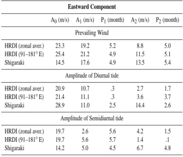
semi-annual (A2, P2). This information is supplied in Table 1 for

the 35◦–40◦N analysis. We concentrate on the HRDI val-ues within the same longitude sector as Shigaraki. For u, Ao

at Shigaraki is 14.5 ms−1, compared to 25.4 ms−1for HRDI in this longitude sector. These lower values for Shigaraki are obviously connected with the lower GB values during

April and July, as noted previously. However, A1 and A2

agree within 20% between GB and SB determinations, and the corresponding phases match almost exactly. For v, the largest component is A1(i.e. 9–10 ms−1), which is about the

same in amplitude for GB vs. SB, but the GB phase leads that of SB by 2.4 months (i.e. 36◦out of 360◦). The GB value of A2is 3.8 ms−1compared to 1.5 ms−1for SB, but the

semian-nual component is of secondary importance for the prevailing meridional wind at this latitude.

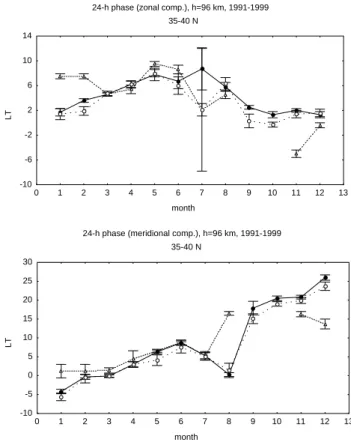
Analogous results for the diurnal tide in this longitude sec-tor are provided in Figs. 3 (amplitude) and 4 (phase) and Table 1. For these and forthcoming results, the seasonal cycles of amplitude and phase for a given tidal component are not fit with annual and semiannual harmonics separately. Rather, these components are written in complex form, the scalar real and imaginary parts are fit separately, and then re-constructed to obtain the amplitudes and phases. Similar to the zonal mean winds, the seasonal cycles of GB/SB zonal wind amplitudes in Fig. 3 agree in terms of salient features, but rather significant differences appear for the meridional winds. GB/SB phase discrepancies occur for a few months (Fig. 4), but for the most part the seasonal variations in di-urnal phase in this latitude regime are in good agreement for both u and v.

The above results are reflected in the annual harmonic am-plitudes (Ao, A1, A2)and phases (P1, P2)in the following

way (see Table 1). For u, the GB Aois 28.9, compared to a

SB value of 21.4; for v, agreement is within 5%. Annual am-plitudes (A1)also agree within 5%, but phase discrepancies

exist (2.2 months for u and 5.6 months for v). A2and P2are

in excellent agreement for v, but the GB A2=14.4 for u far

exceeds the SB value of 3.6 while their phases agree within 1 month.

24-h phase (zonal comp.), h=96 km, 1991-1999 35-40 N month LT -10 -6 -2 2 6 10 14 0 1 2 3 4 5 6 7 8 9 10 11 12 13

24-h phase (meridional comp.), h=96 km, 1991-1999 35-40 N month LT -10 -5 0 5 10 15 20 25 30 0 1 2 3 4 5 6 7 8 9 10 11 12 13

Fig. 4. Same as Fig. 2, except for phase of diurnal tide.

12-h amplitude (zonal comp.), h=96 km, 1991-1999 35-40 N month m/s -5 5 15 25 35 45 0 1 2 3 4 5 6 7 8 9 10 11 12 13

12-h amplitude (meridional comp.), h=96 km, 1991-1999 35-40 N month m/s -5 5 15 25 35 45 0 1 2 3 4 5 6 7 8 9 10 11 12 13

(7)

Table 1. Annual mean, annual (A1, P1) and semiannual (A2, P2) harmonics (amplitude, phase) corresponding to the prevailing (di-urnal mean), di(di-urnal and semidi(di-urnal components of the eastward wind (top) and northward wind (bottom) component for 35◦–40◦N.

Eastward Component

A₀(m/s) A₁(m/s) P₁(month) A₂(m/s) P₂(month) Prevailing Wind

HRDI (zonal aver.) 23.3 19.2 5.2 8.8 5.0 HRDI (91–181◦E) 25.4 21.2 4.9 11.5 5.1

Shigaraki 14.5 17.6 4.9 13.5 5.4

Amplitude of Diurnal tide

HRDI (zonal aver.) 20.9 10.7 .3 2.7 1.7 HRDI (91–181◦E) 21.4 11.1 .3 3.6 3.7

Shigaraki 28.9 11.0 2.5 14.4 2.6

Amplitude of Semidiurnal tide

HRDI (zonal aver.) 19.7 2.6 5.6 4.2 1.5 HRDI (91–181◦E) 19.7 5.6 5.7 1.4 .1

Shigaraki 14.2 5.0 4.5 6.7 4.8

Northward Component

A0(m/s) A1(m/s) P1(month) A2(m/s) P2(month)

Prevailing Wind

HRDI (zonal aver.) −.7 8.8 11.4 1.5 .1 HRDI (91–181◦E) −.1 10.4 11.4 1.5 .5

Shigaraki −1.5 9.3 9.0 3.8 2.9

HRDI (zonal aver.) 16.6 5.4 1.3 3.7 1.7 HRDI (91–181◦E) 17.3 6.1 .5 3.8 2.4

Shigaraki 18.1 5.4 6.1 4.4 2.8

Shigaraki 13.3 10.2 3.0 9.1 5.7

Amplitudes and phases of the semidiurnal tide are pre-sented in Figs. 5 and 6, respectively, and annual harmonics are listed in Table 1. For February–March and June–August, “local” (i.e. for longitude sector 91◦_-181◦_{E) HRDI values} of a2 differ from zonal mean values by 5–10 ms−1,

indicat-ing possibly greater importance of nonmigratindicat-ing tidal com-ponents. The general trend is for the GB amplitudes to agree better with the zonal mean values. There is generally good GB/SB agreement in the annual mean amplitude (20 ms−1), but significant (5–10 ms−1)differences occur during some months. For v there is also reasonable agreement in terms of average amplitude for the year (∼20 ms−1)but the month-to-month GB/SB variations are better correlated than for u. Phases for u oscillate back and forth about a mean value near 07:00 h, which shows only slight variation throughout

12-h phase (zonal comp.), h=96 km, 1991-1999 35-40 N month LT -2 0 2 4 6 8 10 12 14 0 1 2 3 4 5 6 7 8 9 10 11 12 13

12-h phase (meridional comp.), h=96 km, 1991-1999 35-40 N month LT -2 0 2 4 6 8 10 12 0 1 2 3 4 5 6 7 8 9 10 11 12 13

Fig. 6. Same as Fig. 2, except for phase of semidiurnal tide.

the year for SB values. For v, the phase has a linear trend from ∼08:00 to ∼02:00 from beginning to end of the year, whereas the SB phases linearly decrease from ∼05:00 to

∼03:00.

From Table 1, the annual mean semidiurnal amplitude Ao

for u from Shigaraki measurements (14.2 ms−1)

underesti-mates the “local” HRDI value (19.7 ms−1)by about 30%.

GB/SB values of A1 and P1 are in good agreement, while

the GB determination of A2(6.7 ms−1)considerably exceeds

the HRDI value (1.4), and lags the SB value in phase by 4.7 months (i.e. nearly in antiphase). Similar behavior to the above is reflected in v.

General impressions that emerge from the comparisons in Figs. 2–6 are the following. Month-to-month variations in prevailing, diurnal and semidiurnal components derived from SB measurements tends to be smoother and less er-ratic than from the GB winds. This could be due to the in-tegrated sampling offered by the satellite measurements (in terms of latitude, longitude, line of sight), whereas the radar measurements are more localized and perhaps more subject to effects of gravity waves and other geophysical variations. To some extent these differences are ameliorated through examination of annual harmonics of the tidal components. Also, at Shigaraki, the 9-year climatologies are constructed from “campaigns” rather than from a near-continuous data stream like that provided by the Adelaide MF radar. Sec-ondly, the zonal-mean and longitudinally-restricted SB mea-surements seldom disagree within the standard deviations of

(8)

Mean zonal wind, h=96 km, 1991-1999 35-40 S month m/s -20 -10 0 10 20 30 40 50 60 70 0 1 2 3 4 5 6 7 8 9 10 11 12 13

Mean meridional wind, h=96 km, 1991-1999 35-40 S month m/s -20 -15 -10 -5 0 5 10 15 20 0 1 2 3 4 5 6 7 8 9 10 11 12 13

Fig. 7. Climatic season variations of the prevailing zonal (top) and meridional (bottom) wind components at 96 km during 1991–1999 as seen by HRDI and by the MF at Adelaide. Filled circles: HRDI data for the 35◦–40◦S latitude belt, averaged over all longitudes. Open circles: HRDI data for the 93◦–183◦E longitude sector. Open triangles: Adelaide data (35◦S, 138◦E). Vertical bars represent one standard deviation.

the monthly mean values, indicating that nonmigrating tides and stationary planetary waves are not an important consid-eration for SB/GB comparisons in this latitude regime. 3.3 The 35◦_–40◦_{S latitude regime}

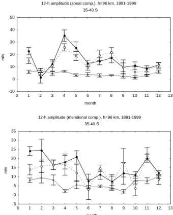
Figures 7–11 depict parameters identical to those in Figs. 2– 6 at the geographically conjugate station of Adelaide (35◦S, 138◦E). The corresponding annual harmonics are tabulated in Table 2. Recall that the radar at Adelaide is an MF spaced-antenna drift radar, whereas the Shigaraki radar is the meteor type. Monthly values of ao for u in Fig. 7 bear some

sim-ilarity to those in Fig. 2, namely maximum winds during summer, with comparatively little variation between spring and fall equinoxes. In fact, near-symmetry between hemi-spheres exists for the SB measurements. At Adelaide, how-ever, the mean value during non-summer months (∼2 ms−1)

is about 10 ms−1 less than the SB measurements and

dur-ing summer months the GB values of ao(∼15–20 ms−1)are

much smaller than the SB values (∼40–50 ms−1). The local (93◦–183◦longitude) and zonal-mean SB values differ little between each other. For v, the three curves practically coin-cide within the limits of the standard deviations, indicating

Table 2. Annual mean annual (A1, P1) and semiannual (A2, P2) harmonics (amplitude, phase) corresponding to the prevailing (di-urnal mean), di(di-urnal and semidi(di-urnal components of the eastward wind (top) and northward wind (bottom) component for 35◦–40◦S.

Adelaide 6.1 7.1 11.2 6.0 4.8

Adelaide 12.5 5.5 3.6 1.4 1.1

HRDI (zonal aver.) 15.3 6.1 3.7 3.6 3.7 HRDI (93–183◦E) 13.5 5.3 4.5 .8 .6

Adelaide 3.5 1.8 1.3 2.2 1.1

Prevailing Wind

HRDI (zonal aver.) 3.7 5.8 .3 2.1 3.3 HRDI (93–183◦E) −.8 7.8 11.8 4.5 3.7

Adelaide 3.0 4.1 11.4 1.6 1.5

Adelaide 7.0 2.7 4.7 1.0 2.1

HRDI (zonal aver.) 15.4 6.4 .9 .4 3.0 HRDI (93–183◦E) 12.7 2.9 .6 2.1 2.3

Adelaide 4.9 3.6 2.0 2.8 1.5

northward winds of ∼5–10 ms−1 during summer reversing

to southward winds of similar amplitude during winter. In addition, there are 5–15 ms−1differences between local and zonal mean values of v from SB measurements, and further-more, in this case the GB measurements agree much more closely with the zonal-mean SB values. All of the above similarities and differences manifest themselves in expected ways in terms of the annual harmonics listed in Table 2.

Figure 8 is the Southern Hemisphere (SH) analogue of Fig. 3 for diurnal tidal amplitudes. Differences between lo-cal and zonal mean SB components are modest, indicating nonmigrating tide contributions of no more than 5–10 ms−1 for u in this longitude sector, and usually less than 5 ms−1 for v. Similar to ao (Fig. 7), monthly variations in the GB

(9)

Table 3. Annual mean annual (A1, P1) and semiannual (A2, P2) harmonics (amplitude, phase) corresponding to the prevailing (di-urnal mean), di(di-urnal and semidi(di-urnal components of the eastward wind (top) and northward wind (bottom) component for 5◦–10◦S.

HRDI (zonal aver.) −11.1 4.0 11.2 7.6 5.3 HRDI (62–152◦E) −12.7 3.4 10.7 8.1 5.3

Jakarta −5.8 .6 3.0 3.2 6.1

HRDI (zonal aver.) 13.7 1.0 2.7 .8 5.6 HRDI (62–152◦E) 17.5 4.5 11.5 2.7 1.4

Jakarta 10.6 1.3 10.2 4.3 5.0

HRDI (zonal aver.) 7.1 2.8 .6 .9 .5 HRDI (62–152◦E) 8.2 1.9 2.4 .8 .7

Jakarta 5.7 1.1 7.6 1.2 1.5

Prevailing Wind

HRDI (zonal aver.) −1.1 6.4 12.0 3.2 5.9 HRDI (62–152◦E) −.2 3.7 1.6 0. 0.

Jakarta −4.7 5.1 11.3 3.6 5.3

Jakarta 12.3 6.4 4.0 1.1 2.1

HRDI (zonal aver.) 19.3 2.5 6.1 2.6 .6 HRDI (62–152◦E) 19.7 3.3 5.1 5.5 1.6

Jakarta 11.2 2.5 6.0 1.7 .1

smaller amplitudes. The differences are less acute for v. In terms of annual mean diurnal amplitudes (Table 2), Ao for

Adelaide (12.5 ms−1)is about 25% less than that for HRDI (16.5 ms−1₎_{for u; for v, the difference is about 20% in the}

same direction. For the next largest (annual) harmonic, A1,

P1 for u and P2for v are in good agreement; however, the

GB value of A2 for v (2.7) underestimates the HRDI value

(5.7) by a factor of 2, although the implications of this differ-ence are minor given the small amplitudes. The GB phases t1

consistently lag the SB phases throughout the year by about 2–6 h while maintaining significant correlation in terms of month-to-month variability. This difference is discussed later in terms of the phase retardation effect thought to exist in MF radar measurements above 90 km; namely, that during the day the reflection height is overestimated. Similar

behav-24-h amplitude (zonal comp.), h=96 km, 1991-1999 35-40 S month m/s -5 5 15 25 35 45 0 1 2 3 4 5 6 7 8 9 10 11 12 13 24-h amplitude (meridional comp.), h=96 km, 1991-1999

35-40 S month m/s -10 0 10 20 30 40 0 1 2 3 4 5 6 7 8 9 10 11 12 13

ior is noted for v phases. During some months, local diurnal phases depart significantly from zonal mean values, possibly indicating effects of nonmigrating components, in contrast to results for the Northern Hemisphere.

Semidiurnal amplitudes (a2) for u (Fig. 10) for the SB

measurements behave similarly to a1 in that maxima occur

during April (35 ms−1)and August (15 ms−1). The Ade-laide GB measurements are small (0–5 ms−1)throughout the

year. For v, GB amplitudes are less than 10 ms−1 during

all months, whereas the local SB values are generally 5– 10 ms−1_{higher, on average. Curiously, seasonal variations}

of semidiurnal phase (Fig. 11) for both u and v are in excel-lent agreement, except for a 1-month later shift in phase for local SB vs. GB measurements around the two equinoxes.

The general result to emerge for 35◦–40◦S is that ampli-tudes of all diurnal harmonics (ao, a1, a2)are significantly

smaller for the Adelaide MF radar measurements compared to those obtained from space. This represents a major differ-ence from the meteor radar results for 35◦_–40◦_{N, and may} be due in part with differences in the radar types. The dif-ferences are consistent with the well-known speed bias for MF radars that was discussed in Sect. 2. In addition, the GB diurnal phases lag the SB phases by several hours; this does not initially appear to be explicable in terms of differences in radar type, but is discussed below in terms of group retar-dation for the MF radar pulses. Semidiurnal phases, on the other hand, are in rather good agreement between GB and SB sources.

(10)

24-h phase (zonal comp.), h=96 km, 1992-1999 35-40 S month LT -2 0 2 4 6 8 10 12 14 16 0 1 2 3 4 5 6 7 8 9 10 11 12 13 24-h phase (meridional comp.), h=96 km, 1991-1999

35-40 S month LT -2 4 10 16 22 28 0 1 2 3 4 5 6 7 8 9 10 11 12 13

3.4 Interannual variability in the ±35◦–40◦ latitude

regimes

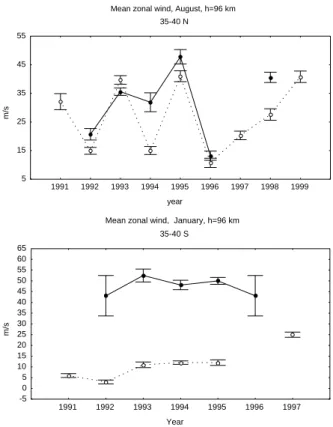
Figures 12–15 compare interannual variability in the SB and GB determinations of prevailing and semidiurnal amplitudes between 35◦_–40◦_{N and 35}◦_–40◦_{S during the months of} Au-gust and January, the local summer solstice months. Interan-nual variations in prevailing u during August in the NH are substantial (∼10–40 ms−1), and track reasonably well be-tween GB and SB measurements. However, in the SH for January, interannual variability is small, and there is a large

difference between mean GB (∼10 ms−1) and SB (∼40–

50 ms−1)values. As discussed further in Sect. 4, overesti-mation of the reflection height during daytime by MF radars may explain this difference. For the mean zonal wind during summer, 96 km is in a region of strong positive shear due to the deposition of eastward momentum by gravity waves. If the actual reflection height is lower than that inferred, then the MF radar winds will underestimate the true winds. The shear in the meridional wind is less than that of the zonal, consistent with the GB/SB differences between Figs. 12 and 13.

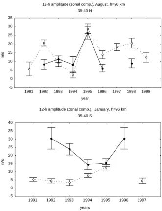
Figures 14 (for u) and 15 (for v) depict similar results for the semidiurnal tide. At 35◦−40◦N, GB values of a2 for

u mimick the salient features in the SB values, with some deviations in 1992 and 1998. At 35◦−40◦S, however, sig-nificant GB/SB differences are evident, with GB values un-derestimating SB, and interannual SB and GB variations in a2being anticorrelated. For v, the Northern Hemisphere GB

12-h amplitude (zonal comp.), h=96 km, 1991-1999 35-40 S month m/s -10 0 10 20 30 40 50 0 1 2 3 4 5 6 7 8 9 10 11 12 13

12-h amplitude (meridional comp.), h=96 km, 1991-1999 35-40 S month m/s -5 0 5 10 15 20 25 30 35 0 1 2 3 4 5 6 7 8 9 10 11 12 13

Fig. 10. Same as Fig. 7, except for amplitude of semidiurnal tide.

12-h phase (zonal comp.), h=96 km, 1991-1999 35-40 S month LT 2 4 6 8 10 12 14 16 0 1 2 3 4 5 6 7 8 9 10 11 12 13

12-h phase (meridional comp.), 96 km, 1991-1999 35-40 S month LT -8 -4 0 4 8 12 16 20 0 1 2 3 4 5 6 7 8 9 10 11 12 13

(11)

Mean zonal wind, August, h=96 km 35-40 N year m/s 5 15 25 35 45 55 1991 1992 1993 1994 1995 1996 1997 1998 1999 Mean zonal wind, January, h=96 km

35-40 S Year m/s -5 0 5 10 15 20 25 30 35 40 45 50 55 60 65 1991 1992 1993 1994 1995 1996 1997

Fig. 12. Year-to-year variability of the monthly mean zonal wind at 96 km during 1991–1999 as seen by HRDI and ground-based instruments. Filled circles: HRDI data for 35◦–40◦N for August (top) and 35◦–40◦S for January (bottom). Open circles: the cor-responding data at Shigaraki (35◦N, 136◦E) and Adelaide (35◦S, 138◦E). Vertical bars represent one standard deviation.

variations capture the salient features of interannual variabil-ity depicted by the SB values. Again, GB values in the South-ern Hemisphere are smaller than the SB a2s, and show

rela-tively little interannual variability in comparison. 3.5 The 5◦_–10◦_{S latitude regime}

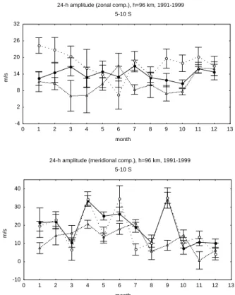
Figures 16–20 and Table 3 provide the same information in Figs. 2–6 and 7–11 and Table 2, respectively, except for the meteor radar at Jakarta (6◦_{S, 107}◦_{E). The SB prevailing} zonal winds ao(Fig. 16) do not indicate the presence of any

significant longitude dependence (i.e. high-amplitude sta-tionary waves ). While aofor the SB measurements indicates

maxima in July (∼−5 ms−1)and December (∼+5 ms−1)and minima (∼ − 20 ms−1)at the equinoxes (i.e. a semiannual variation), the GB values do not deviate much from ±5 ms−1.

Thus, GB/SB differences of the order of 10–15 ms−1 are

common throughout the year, consistent with the factor of

∼2 difference in A0for u in Table 3. GB values of aofor v

agree well with local SB values, except during March, May and August, where differences of 10–20 ms−1exist.

SB diurnal amplitudes (Fig. 17) reflect significant dif-ferences between local and zonal mean values, indicating possible presence of nonmigrating diurnal tides (cf. Ta-laat and Lieberman, 1999; Forbes et al., 2003; Manson

Mean meridional wind, August, h=96 km 35-40 N year m/s -30 -25 -20 -15 -10 -5 0 5 10 1991 1992 1993 1994 1995 1996 1997 1998 1999

Mean meridional wind, January,h=96 km 35-40 S years m/s -5 0 5 10 15 20 25 30 35 1991 1992 1993 1994 1995 1996 1997

Fig. 13. Same as Fig. 12, except for the meridional wind compo-nent.

et al., 2002). For both the zonal and meridional diurnal amplitudes, GB/SB discrepancies in the range of 5–12 ms−1 occur throughout the year. On average, GB/SB amplitude ratios are ∼0.6 for the u component and ∼0.7 for the v com-ponent (see Table 3). Diurnal phases are in reasonable agree-ment, however, with the exception of ∼8-h phase discrepan-cies in March, April, July and August for u, and May, July and December for v.

For the semidiurnal amplitudes (Fig. 19) GB values of a2

for u generally agree with SB values within the uncertainty estimates, except during March, June, August and

Decem-ber, where ∼5–10 ms−1 _{differences are noted. For v, GB}

values are, on average, ∼0–10 ms−1_{less than SB amplitudes,}

with an average GB/SB ratio of ∼0.6 (Table 3). Semidiurnal phases are in agreement (Fig. 20) in terms of magnitude and trends, within the standard deviation limits.

4 Summary and conclusions

In this work comparisons were performed between monthly climatological prevailing and tidal wind fields at 96 km from the HRDI instrument on UARS and those from GB radar measurements. The primary intent was to provide a perspec-tive alternaperspec-tive to the overflight comparisons that have been conducted to date, and to provide context and guidance to future efforts as part of TIMED and other future aeronomy missions.

(12)

12-h amplitude (zonal comp.), August, h=96 km 35-40 N year m/s -5 0 5 10 15 20 25 30 35 1991 1992 1993 1994 1995 1996 1997 1998 1999 12-h amplitude (zonal comp.), January, h=96 km

35-40 S years m/s -5 0 5 10 15 20 25 30 35 40 1991 1992 1993 1994 1995 1996 1997

The GB data investigated here originate from meteor radars at Obninsk, (55◦_{N, 37}◦_{E), Shigaraki (35}◦_{N, 136}◦_E) and Jakarta (6◦_{S, 107}◦_{E) and MF spaced-antenna radars at} Hawaii (22◦N, 160◦W), Christmas I. (2◦N, 158◦W) and

Adelaide (35◦S, 138◦E). Taking the monthly zonal mean

winds from these stations as a whole, HRDI SB zonal winds exceed GB radar wind determinations by ∼63%. This re-sult is consistent with conclusions made by Portnyagin et al. (1999), inferred by comparing wind measurements from the WINDII instrument on UARS with a radar-based global empirical wind model. In the present study, GB and SB meridional winds agree on average (i.e. statistically), but the scatter is considerable. Origins of the discrepancy for the zonal wind component remain unknown, and evidence for this effect should be pursued early within the TIMED SB/GB program.

A study of winds from the conjugate stations of Shigaraki and Adelaide was conducted, with the following results:

1. For prevailing zonal winds, GB/SB agreement is excel-lent at Shigaraki, except for the months of April and Au-gust. At Adelaide, prevailing winds are a factor of 2–3 less than SB values, although the variations track well. On the other hand, in the presence of significant scat-ter, there are no consistent SB/GB differences at Shi-garaki or Adelaide for the prevailing meridional com-ponent, although important discrepancies exist during some months.

12-h amplitude (meridional comp.), August, h=96 km 35-40 N year m/s -2 4 10 16 22 28 34 1991 1992 1993 1994 1995 1996 1997 1998 1999

12-h amplitude (meridional comp.), January,h=96 km 35-40 S years m/s -5 5 15 25 35 45 55 1991 1992 1993 1994 1995 1996 1997

2. At Shigaraki, diurnal amplitudes for the zonal wind agree well with SB values, except during August; smaller differences (∼30%) also exist in November and December. The correspondence is not as good for the meridional component, with significant (∼100%) dif-ferences existing during almost half the months, but no consistent trend is noted. At Adelaide, diurnal and semidiurnal GB amplitudes are consistently less than their SB counterparts, ∼0.7 and ∼0.4, respectively, av-eraged over the year. Diurnal phases are broadly consis-tent between SB/GB values at Shigaraki, but at Adelaide the diurnal wind maxima consistently lag behind the SB values by ∼4 h, on average.

3. For the semidiurnal tide the standard deviations are larger. Shigaraki amplitudes are of the same order of magnitude as SB values, and phases vary considerably about quasi-steady SB phases. The Adelaide radar sig-nificantly underestimates SB semidiurnal amplitudes, especially the zonal wind component, but phases are in excellent agreement.

4. Interannual variations between SB/GB winds measured at the conjugate sites of Shigaraki and Adelaide are markedly different. Zonal mean and semidiurnal am-plitudes at Shigaraki capture absolute magnitudes and track salient variations in the HRDI measurements rea-sonably well. At Adelaide, average amplitudes and in-terannual trends are significantly different from those revealed in the SB measurements. Although differences

(13)

Mean zonal wind, h=96 km, 1991-1999 5-10 S month m/s -30 -20 -10 0 10 0 1 2 3 4 5 6 7 8 9 10 11 12 13

Mean meridional wind, h=96 km, 1991-1999 5-10 S month m/s -25 -15 -5 5 15 25 0 1 2 3 4 5 6 7 8 9 10 11 12 13

Fig. 16. Climatic seasonal variations of the prevailing zonal (top) and meridional (bottom) wind components at 96 km during 1991– 1999 as seen by HRDI and by the meteor radar at Jakarta. Filled circles: HRDI data for the 5◦–10◦S latitude belt, averaged over all longitudes. Open circles: HRDI data for the 62◦–152◦E longitude sector. Open triangles: Jakarta data (6◦S, 107◦E). Vertical bars represent one standard deviation.

in radar type could possibly account for some instru-mental biases, it seems unlikely that instruinstru-mental effects could explain differences in interannual trends.

The lag between radar measurements of tidal phase at Adelaide and those by the HRDI instrument are consistent with phase retardation effects in the MF radar technique. When background ionization levels are sufficiently high (i.e. low solar zenith angles), wave retardation yields an overes-timate of the reflection height. Since upward-propagating waves are characterized by downward phase progression, the calculated phase (with a later local time) corresponds to a lower height than the measured reflection height. The ∼4-h phase difference depicted in Fig. 9 for the diurnal tide im-plies a reflection height error of ∼4 km for a 25-km verti-cal wavelength oscillation. The absence of such a phase lag for the semidiurnal tide is consistent with the longer wave-lengths expected for the 12-h oscillation. As noted previ-ously in connection with Figs. 12 and 13, the retardation ef-fect is also manifested in underestimates of the prevailing zonal and meridional winds at 96 km during local summer months, due to the large positive shears that exist under these conditions. The phase retardation effect, in addition to the well-established speed bias for MF radars, is consistent with

24-h amplitude (zonal comp.), h=96 km, 1991-1999 5-10 S month m/s -4 2 8 14 20 26 32 0 1 2 3 4 5 6 7 8 9 10 11 12 13

24-h amplitude (meridional comp.), h=96 km, 1991-1999 5-10 S month m/s -10 0 10 20 30 40 0 1 2 3 4 5 6 7 8 9 10 11 12 13

the trends and bias noted in the Adelaide/Shigaraki compari-son. It is also noted that this speed bias (noted in the context of receiver saturation by Vincent, 1995) also exists in sys-tems that do not have a receiver saturation problem (Nam-boothiri et al., 1993; Nozawa et al., 2002).

The Jakarta GB/SB comparisons show some features dif-ferent from those of the Adelaide/Shigaraki comparison. First, differences between zonal mean and local determi-nations of the diurnal tide are often significant, indicating the presence of nonmigrating tides. This result is consistent with other analyses of UARS wind measurements (Talaat and Lieberman, 1999; Forbes et al., 2003; Manson et al., 2002). Second, a consistent speed bias exists, indicating SB/GB ra-tios of the order of 1.6 for the prevailing wind and 1.3 for the semidiurnal tide. Given that both the Shigaraki and Jakarta radars are of the meteor type, it is surprising that the GB/SB ratios are so much smaller for Shigaraki. The Jakarta tidal phases are often in good agreement, yet significant differ-ences exist for 3–4 months of the year. Neither of these as-pects of our GB/SB comparisons is understood, but remain relevant for any future studies that seek to assimilate GB and SB data together in any kind of model.

The origins of other GB/SB differences noted in the present work may arise from several sources. Particularly prominent may be inadequate sampling in time and space of a flow that is nonstationary and spatially inhomogeneous. Effects of gravity waves, planetary waves, intraseasonal and interannual variations may all be important contributors. The significant interannual variability depicted in Figs. 12–15

(14)

24-h phase (zonal comp.), h=96 km, 1991-1999 5-10 S month LT -10 -6 -2 2 6 10 14 18 0 1 2 3 4 5 6 7 8 9 10 11 12 13

24-h phase (meridional comp.), h=96 km, 1991-1999 5-10 S month LT -4 2 8 14 20 26 0 1 2 3 4 5 6 7 8 9 10 11 12 13

emphasize this latter point. Irregardless of the origin, such differences remain an important consideration for GB/SB data assimilation. Remember that SB estimates of tidal am-plitudes and phases were made by averaging all data within 10◦×90◦latitude × longitude sectors centered on the latitude and longitude of the radar site, whereas GB estimates almost correspond to point measurements by comparison. More-over, one must not forget the reason why GB and SB data provide such complementary perspectives on the dynamical flow field: GB data are characterized by excellent temporal coverage while SB data provide near-global spatial coverage. It is these characteristics exactly that make intercalibration of data from these two sources so difficult.

4.1 Recommendations for future missions

The following recommendations for TIMED and other future missions emerge from our findings:

1. It must be established as soon as possible whether the anisotropy between SB/GB comparisons of the zonal vs. meridional components of the wind field revealed here and in Portnyagin et al. (1999) is repeated, and to uncover the reasons.

2. Perform comparisons at 90 km, where differences be-tween MF and meteor radar techniques are minimized. 3. More frequent sampling by SB instruments is

re-quired (i.e. 100% duty cycle) to enable shorter (i.e.

12-h amplitude (zonal comp.), h=96 km, 1991-1999 5-10 S month m/s -6 0 6 12 18 24 0 1 2 3 4 5 6 7 8 9 10 11 12 13

12-h amplitude (meridional comp.), h=96 km, 1991-1999 5-10 S month m/s 0 10 20 30 40 0 1 2 3 4 5 6 7 8 9 10 11 12 13

12-h phase (zonal comp.), h=96 km, 1991-1999 5-10 S month LT 0 2 4 6 8 10 12 14 0 1 2 3 4 5 6 7 8 9 10 11 12 13

12-h phase (meridional comp.), h=96 km, 1991-1999 5-10 S month LT 0 2 4 6 8 10 12 14 0 1 2 3 4 5 6 7 8 9 10 11 12 13

(15)

individual-year) and more localized (i.e. 5◦_{latitude ×} 15◦_{longitude) volumes for climatological comparisons.} 4. For missions with slower local time precession rates than UARS, determinations of tides from SB measure-ments alone will be smeared due to time evolution of the dynamics within the fit span. In this case, the pre-ferred means of GB/SB comparison may lie in “local time space” in the climatological sense, i.e. in con-junction with each GB site, monthly mean values of eastward and northward wind components should be

formed within 5◦ latitude × 30◦ longitude × 2-h

lo-cal time bins. Comparisons would be made with similar monthly mean values from the radar or optical site. This eliminates the need for acquiring data over a sufficiently long local time span to extract diurnal and semidiurnal harmonics, while still retaining the advantages of a cli-matological comparison.

5. For the TIMED Mission, the ideal location for perform-ing SB/GB comparisons of MLT wind measurements will be the South Pole. Due to the combination of view-ing geometry and orbital inclination, the TIDI instru-ment will measure winds over the South Pole on every orbit. A meteor radar system now exists at the South Pole that is capable of providing wind measurements (between 80 and 100 km) complementary to that of the TIDI instrument. This fortunate circumstance will allow both coincident and climatological comparisons to be conducted, minus many of the shortcomings normally associated with each methodology.

Acknowledgements. This work was supported under NASA Grants NAG5-8755 and NAG5-5028 to the University of Colorado. The authors thank the referees for comprehensive and authoritative re-views of our work.

Topical Editor U.-P. Hoppe thanks A. Manson and another ref-eree for their help in evaluating this paper.

References

Burrage, M. D., Arvin, N., Skinner, W. R., and Hays, P. B.: Obser-vations of the O2atmospheric band nightglow by the High

Res-olution Doppler Imager, J. Geophys. Res., 99, 15 017–15 023, 1994.

Burrage, M. D., Skinner, W. R., Gell, D. A., Hays, P. B., Marshall, A. R., Ortland, D. A., Manson, A. H., Franke, S. J., Fritts, D. C., Hoffman, P., McLanderess, C., Nicijewski, R., Schmidlin, F. J., Shepherd, G. G., Singer, W., Tsuda, T., and Vincent, R. A.: Validation of mesosphere and lower thermosphere winds from the high-resolution Doppler imager on UARS, J. Geohphys. Res., 101, 10 365–10 392, 1996.

Cervera, M. A. and Reid, I. M.: Comparison of simultaneous wind measurements using co-located VHF meteor radar and MF spaced antenna radar systems, Radio Sci., 30, 1245–1261, 1995. Forbes, J. M., Jarvis, M. J., Palo, S. E., Zhang, X., Portnyagin, Yu. I., and Makarov, N. A.: Electric fields and meteor radar wind measurements near 95 km over South Pole, Adv. Polar Upper At-mos. Res., 15, 1–10, 2001.

Forbes, J. M., Zhang, X., Ward, W., and Talaat, E.: Nonmigrating diurnal tides in the thermosphere, J. Geophys. Res., 108, 1033, doi:10.1029/2002JA009262, 2003.

Hays, P. B., Abreu, V. J., Dobbs, M. E., Gell, D. A., Grassl, H. J., and Skinner, W. R.: The High Resolution Doppler Imager on the Upper Atmosphere Research Satellite, J. Geophys. Res., 98, 10 713–10 723, 1993.

Hocking, W. K.: Strengths and limitations of MST radar measure-ments of middle-atmosphere winds, Ann. Geophys., 15, 1111– 1122, 1997.

Hocking, W. K. and Thayaparan, T.: Simultaneous and co-located observations of winds and tides by MF and meteor radars over London, Canada (43◦N, 81◦W) during 1994–1996, Radio Sci., 32, 833–865, 1997.

Hocking, W. K., Fuller, B., and Vandepeer, B.: Real-time deter-mination of meteor-related parameters utilizing modern digital technology, J. Atmos. Sol. Terr. Phys., 63, 155–169, 2001. Kendall, M. G. and Stuart, A.: The Advanced Theory of

Statis-tics, v. 2, Inference and Relationship, Charles Griffin & Com-pany Ltd., London, 1966.

Lieberman, R. S., Robinson, W. A., Franke, S. J., and Vincent, R. A. et al.: HRDI observations of mean meridional winds at solstice, J. Atmos. Sci., 55, 1887–1896, 1998.

Manson, A. H., Yi, F., Hall, G., and Meek, C.: Comparisons Between Instantaneous Wind Measurements Made at Saska-toon (52◦N, 107◦W) Using the Co-located Medium Frequency Radars and Fabry-Perot Interferometer Instruments: Climatolo-gies (1988–1992) and Case Studies, J. Geophys. Res., 101, 29 553–29 563, 1996.

Manson, A. H., Luo, Y., and Meek, C.: Global Distributions of Di-urnal and semi-DiDi-urnal Tides: Observations from HRDI-UARS of the MLT Region, Ann. Geophys., 20, 1877–1890, 2002. Manson, A. H., Meek, C. E., Brekke, A., and Moen, J.: Mesosphere

and lower thermosphere (80–120 km) winds and tides from near Tromsø (70◦N, 19◦E): Comparisons between radars MF, EIS-CAT, VHF and rockets, J. Atmos. Terr. Phys., 54, 927–950, 1992. Manson, A. H., Meek, C. E., Hall, C. M., Nozawa, S., Mitchell, N. J., Pancheva, D., Singer, W., and Hoffmann, P.: Mesopause Dynamics from the Scandinavian Triangle of Radars within the PSMOS-DATAR Project, Ann. Geophys., 22(2), 367–386, 2004. Meek, C. E., Manson, A. H., Burrage, M. D., Garbe G., and Cog-ger, L. L.: Comparisons Between Canadian Prairie MF Radars, FPI (green and OH Lines) and UARS HRDI Systems, Ann. Geo-phys., 15, 1099–1110, 1997.

Nakamura, T., Tsuda, T., Tsutsumi, M., Kita, K., Uehara, T., Kato, S., and Fukao, S.: Meteor wind observations with the MU radar, Radio Sci., 26, 857–869, 1991.

Nakamura, T., Tsuda, T., and Tsutsumi, M.: Development of an external interferometer for meteor wind observation attached to the MU radar, Radio Sci., 32, 1203–1214, 1997.

Namboothiri, S. P., Manson, A. H., and Meek, C. E.: E-Region Real Heights and their Implications for MF Radar-derived Wind and Tidal Climatologies, Radio Sci., 28, 187–202, 1993.

Nozawa, S., Brekke, A., Manson, A. H., Hall, C. M., Meek, C., Morise, K., Oyama, S., Dobashi, K., and Fujii, R.: A comparison study of the auroral lower thermospheric neutral winds derived by the EISCAT UHF radar and the Tromso medium frequency radar, J. Geophys. Res., 107, doi:10.1029/2000JA007581, 2002. Portnyagin, Yu. I. and Solovjova, T. V.: Global empirical wind model for the upper mesosphere/lower thermosphere, I. Prevail-ing wind, Ann. Geophys., 18, 300–315, 2000.

(16)

Portnyagin, Yu. I., Solovjova, T. V., and Wang, D. Y.: Some results of comparison between the lower thermosphere zonal winds as seen by the ground-based radars and WINDII on UARS, Earth, Planets and Space, 51, 701–709, 1999.

Shepherd, G. G., Thullier, G., Gault, W. A., and Solheim, B. H. et al.: WINDII: The Wind Imaging Interferometer on the Upper Atmosphere Research Satellite, J. Geophys. Res., 98, 10 725– 10 750, 1993.

Talaat, E.R., and Lieberman, R.S., Nonmigrating diurnal tides in mesospheric and lower-thermospheric winds and temperatures, J. Atmos. Sci., 56, 4073-4087, 1999.

Thayaparan, T. and Hocking, W. K.: A long-term comparison of winds and tides measured at London, Canada (43◦N, 81◦W) by collocated MF and meteor radars during 1994–1999, J. Atmos. Solar-Terr. Phys., 64, 931–946, 2002.

Valentic, T. A., Avery, J. P., Avery, S. K., and Vincent, R. A.: A comparison of winds measured by meteor radar systems and an MF radar at Buckland Park, Radio Sci., 32, 867–874, 1997. Vincent, R. A., Holdsworth, D. A., Reid, I. M., and Cervera, M.

A.: Spaced-antenna wind measurements: The effects of signal saturation, Proc. Wind Observations in the Middle Atmosphere Workshop, Cent. Natl. d’Etudes Spatiales, Paris, 1995.