A Distributionally Robust Approach to Black-Box Optimization
The MIT Faculty has made this article openly available.
Please share
how this access benefits you. Your story matters.
Citation
Kapteyn, Michael G., et al. "A Distributionally Robust Approach to
Black-Box Optimization." 2018 AIAA Non-Deterministic Approaches
Conference, 8-12 January, 2018, Kissimmee, Florida, American
Institute of Aeronautics and Astronautics, 2018.
As Published
https://doi.org/10.2514/6.2018-0666
Publisher
American Institute of Aeronautics and Astronautics
Version
Author's final manuscript
Citable link
http://hdl.handle.net/1721.1/116646
Terms of Use
Creative Commons Attribution-Noncommercial-Share Alike
A Distributionally Robust Approach to Black-Box
Optimization
Michael G. Kapteyn
⇤and Karen E. Willcox
†Massachusetts Institute of Technology, Cambridge, Massachusetts, USA, 02139
Andy B. Philpott
‡University of Auckland, Auckland, New Zealand, 1010
Deciding how to represent and manage uncertainty is a vital part of designing complex systems. Widely used is a probabilistic approach—assigning a probability distribution to each uncertain variable. However, this presents the designer with the task of assuming or estimating these probability distributions from data; a task which is inevitably prone to error. This paper addresses this challenge by formulating a distributionally robust design optimization problem, and presents computationally efficient algorithms for solving the problem. In distributionally robust optimization (DRO) methods, the designer acknowl-edges that they are unable to exactly specify a probability distribution for the uncertain variables, and instead specifies a so-called ambiguity set of possible distributions. This paper uses an acoustic horn design problem to explore how the error incurred in estimat-ing a probability distribution from data a↵ects the realized performance of designs found using a traditional multi-objective optimization under uncertainty. It is found that placing some importance on a risk reduction objective results in designs that are more robust to these errors, and thus have a better mean performance realized under the true distribution than if the designer were to focus all e↵orts on optimizing for mean performance alone. In contrast, the DRO approach is able to uncover designs that are not attainable using the multi-objective approach when given the same data. These DRO designs in some cases significantly outperform those designs found using the multi-objective approach.
I.
Introduction
In designing a system to achieve optimal performance, the designer typically evaluates system performance using some quantity of interest (e.g., cost, efficiency, or weight). Underlying parameters and variables of the system a↵ect the performance of the system, yet in any real-world system, some of these parameters will be uncertain. In this paper, we explore how imperfect representations of these uncertainties can cause traditional optimization under uncertainty methods to produce designs that perform poorly when realized under the true distribution of uncertainty. We then show how a novel formulation of the design problem as a Distributionally Robust Optimization (DRO) addresses this issue by finding designs that are robust to deviations in the distribution of the uncertainty. We then present computationally efficient algorithms for solving the DRO problem and show that our method outperforms a traditional multi-objective optimization method.
Mathematically, we represent the quantity of interest as a function Z(x, u) where x2 X is a vector of design variables that belongs to the design spaceX , and u 2 U is a vector of uncertain variables that belong to the uncertainty spaceU. The problem of design optimization under uncertainty is thus to find a set of optimal design variables x⇤that minimize (or maximize, depending on the application) this function.
⇤S.M. Candidate, Department of Aeronautics and Astronautics. AIAA Student Member. †Professor, Department of Aeronautics and Astronautics. AIAA Associate Fellow. ‡Professor, Department of Engineering Science.
This can be expressed mathematically as min
x2XZ(x, u), u2 U. (1)
Computational modeling of the system of interest provides the designer a means to cheaply and rapidly explore how changes in the underlying parameters a↵ect the output quantity of interest, and thus supports more informed design decisions. In this work, we consider the setting in which the designer has access to a high-fidelity computational model of the system of interest, which takes as input the variables x and values for the uncertain parameters u, and returns an accurate evaluation of the quantity of interest Z(x, u). In practice, such computational models are often complex, proprietary, legacy, and/or written in poorly documented code that the designer may not have time to decipher. With these settings in mind, in this paper we treat the model as a black-box system, assuming no knowledge of the model structure or the behavior of the output variable and its functional relationship to input variables. This makes the design methodology discussed herein general in the sense that it is agnostic to the specific details or formulation of the computational model.
The importance of considering the uncertain nature of the parameters u has long been established,1–3 the
primary reason being that methods that simply consider all parameters to be deterministic tend to over-fit designs to the chosen parameter values. This often results in degraded performance of the system when it is exposed to the true uncertain operating environment.4, 5 A major point of di↵erence among optimization
under uncertainty approaches developed in recent years is in their treatment of these uncertain parameters. The first decision a designer must make is in how to characterize and represent the uncertainty. The most prevalent approach is to treat the uncertain parameters as random variables, with each parameter being assigned a probability distribution according to which it varies.1, 4 Other treatments and representations of
uncertainty have also been established,6such as interval or set-based uncertainty,7–9 and possibility theory.10
Although each of these treatments have their respective merits and drawbacks, one common fact is that the designer is always required to specify something about the uncertain parameters. In this paper we focus on the case of probabilistic uncertainties, where the designer must specify a probability distribution for the uncertain parameters. In practice the designer will never have access to the exact distribution of an uncertain parameter. Consequently, the designer will be forced to assume a probability distribution or to estimate it from known data; processes that will always be prone to error. The subsequent optimization of a design to perform well under this erroneous distribution will often lead to worse than expected performance when the design is realized under the true distribution. In Section II we explore this problem concretely using a practical design optimization under uncertainty case study, and show how the error introduced in specifying probabilistic uncertainties a↵ects the performance of the resulting optimal designs when realized under the true distribution.
Recently, a body of work has emerged from within the optimization community studying an approach that explicitly accounts for the fact that one is never able to exactly specify a probability distribution.11–16
This approach, called Distributionally Robust Optimization, weakens the assumption of specifying a single probability distribution for the uncertain parameters, and instead only requires the designer to select a set of possible probability distributions which is assumed to contain the true distribution. In Section III we describe this approach in detail, and formulate a distributionally robust design optimization problem, applicable to black-box models. We present novel algorithms that solve the resulting problem in a computationally efficient way, requiring practically the same computational budget as traditional design optimization problems. We then provide results which show that, when provided the same data on the uncertain variables, the DRO approach produces designs that outperform those obtained using a traditional multi-objective optimization (MOO) approach. Finally in Section V we conclude the paper and suggest areas to explore in future work.
II.
Motivating problem: Mean-Risk Tradeo↵ via Multi-Objective
Optimization
Assumptions on the form and parameters defining the distributions for probabilistic uncertainties a↵ect the performance of designs found using optimization under uncertainty methods. In order to illustrate this impact, this section presents an illustrative design under uncertainty problem. In Section II.A we formulate the problem of designing an acoustic horn subject to an uncertain operating condition. Section II.B formulates a multi-objective optimization problem to jointly optimize the mean and risk of the horn design. Finally, Section II.C demonstrates how errors in the definition of the distribution of the uncertain operating condition a↵ect the performance of the resulting optimal designs.
II.A. Problem Formulation: Design of an Acoustic Horn
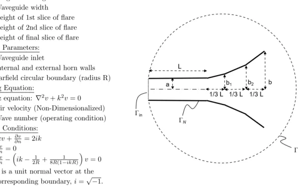
We suppose that we are tasked with optimizing the design of an acoustic horn in order to minimize the amount of internal reflection present, and thus maximize the efficiency of the horn. A computational model allows us to compute a measure of the internal reflection, and thus the performance of a horn for a given geometry, when operating at a given wave number. A brief summary of the model is presented in Figure 1 below. For more details on the model, we refer the reader to Ng and Willcox17 and the references therein.
Geometric Parameters:
L = Length of waveguide and flare a = Waveguide width
b1= Height of 1st slice of flare
b2= Height of 2nd slice of flare
b = Height of final slice of flare Boundary Parameters:
in= Waveguide inlet
N= Internal and external horn walls R= Farfield circular boundary (radius R)
Governing Equation:
Helmholtz equation: r2v + k2v = 0
v = Air velocity (Non-Dimensionalized) k = Wave number (operating condition) Boundary Conditions: in: ikv +@n@v = 2ik N: @n@v = 0 R: @n@v ⇣ ik 2R1 +8R(1 ikR)1 ⌘v = 0 Note: n is a unit normal vector at the
corresponding boundary, i =p 1.
Figure 1: A summary of the acoustic horn model.18
The governing equation is solved to compute the air velocity, v, using a reduced basis finite element model with n = 100 basis vectors. The output of the model is the reflection coefficient:
s = Z
in
v d 1 (2)
which is a fractional measure describing how much a wave is internally reflected in the horn, versus being transmitted out into the environment. It is thus considered a measure of the horn efficiency, with a lower reflection coefficient giving more favorable performance. For this study, we consider the case where the design variables are the two internal flare heights, b1 and b2(Fig. 1), while the uncertain parameter is the operating
wave number k. The remaining parameters are considered fixed so that, in the notation of Section I, we have: Design Variables Uncertain parameters Output Quantity of Interest
x = " b1 b2 # u = k Z(x, u) = s For this case study, the wave number follows a fixed truth probability distribution
u⇠ u= Uniform(1.3, 1.5). (3)
To begin with, we will proceed under the assumption that we as designers know the exact form of u. Later
we will argue that this is in fact never the case in practice, and show what happens when we instead have imperfect knowledge of the distribution u.
II.B. The Multi-Objective Approach
In order to find designs that account for the uncertainty in the wave number, we will employ a multi-objective approach. Our first multi-objective will be to minimize the expected performance under the wave number distribution u. Our second objective will be to minimize a measure of the risk level of a design. The
measure we adopt is perhaps the simplest risk measure: the standard deviation in performance under u.
Adding a risk minimization objective of this type allows us to avoid horn designs with extreme variability in performance over the range of wave numbers, in e↵ect avoiding designs with extremely poor worst-case performance.
The multi-objective optimization problem for mean and standard deviation can be written as min x2X (1 )µ + (4) where µ = u[Z(x, u)] , 2 = u ⇥ (Z(x, u) µ)2⇤, 2 [0, 1]
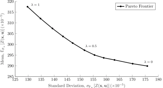
and u denotes the expectation under the distribution u. This type of multi-objective optimization has been studied extensively (see, e.g., Ref. 19–23), and can be solved for any permissible value of to generate a Pareto optimal design. The set of Pareto optimal designs forms a mean-risk trade-o↵ curve called the Pareto frontier. The Pareto frontier for the acoustic horn design problem is shown in Figure 2. A key limitation
125 130 135 140 145 150 155 160 165 170 175 180 285 290 295 300 305 310 315 320 = 0 = 0.5 = 1
Standard Deviation, u[Z(x, u)] (⇥10
5) M ean , u [Z (x ,u )] (⇥ 10 5) Pareto Frontier
Figure 2: Pareto frontier in the mean-risk trade space for the acoustic horn design problem. of the multi-objective problem used to generate the Pareto frontier given in Figure 2 is that it requires exact knowledge of the probability distribution ugoverning the uncertain wave number. This allowed us
to precisely compute the mean and standard deviation in performance under this distribution, and thus minimize these measures directly. In practice, the designer will not have knowledge of the exact distribution of the wave number. Consequently, the designer will be forced to make an assumption about the probability distribution, with unknown impacts on the resulting optimal design.
Fortunately the designer rarely has to make this assumption blindly. Instead, the designer usually has some knowledge about certain features of the uncertainty. In this case we say the designer has partial observability over the uncertainty. For example, the designer might know that the wave number varies between 1.3 and 1.5. In this case the designer knows the support of the distribution. Alternatively the designer might know that the variation in wave number is symmetric and centered around 1.4. In this case they have knowledge about the symmetry and mean of the distribution. Another situation that commonly arises in practice is
where the designer has no knowledge of features about the distribution itself, but instead has access to a finite number of sampled values from the distribution. In our setting, this would be the case if the designer were able to take a finite number of measurements of the wave number as it varied over time (according to the true but unknown distribution u). We will consider this scenario, denoting by m the number of samples
(measurements) to which the designer has access.
In this setting, a commonly used approach is to approximate the true distribution uusing the empirical
distribution ˆp associated with the samples. In this case ˆpidenotes the likelihood that the uncertain parameters
take the values ui. Thus, the mean and standard deviation of the performance under u are approximated
using the mean and the standard deviation of the performance evaluated at the sampled uncertainty values ui for i = 1, .., m. This approach is chosen since the empirical distribution is expected to converge to the
true distribution (for most well-behaved distributions encountered in practice) as m ! 1. Under this approximation, the minimization statement (4) now becomes
min x2X (1 )ˆµ + ˆ (5) where ˆ µ = m X i=1 ˆ piZ(x, ui), ˆ2 = m X i=1 ˆ pi(Z(x, ui) µ)ˆ 2, 2 [0, 1].
We solve the multi-objective optimization problem with sampled uncertainty using a subgradient descent method, which is outlined in Algorithm 1 below. This algorithm utilizes the computational model of the acoustic horn to compute the reflection coefficient Z for a given design x, at each sampled value of the uncertainty ui. We then use the derivative of the reflection coefficient with respect to design variables to
move the design in the direction that improves the objective function in Eq. (5). This is repeated until the design x converges to within a desired tolerance. We choose the gradient descent step-size ↵(j) at iteration j
of the optimization based on the square summable but not summable criterion,24 setting ↵(j)= 1/j.
II.C. Performance of the Multi-Objective Approach Under Partial Observability
We now investigate how the multi-objective approach performs for various sample sizes m of the uncertain wave number in the acoustic horn design problem described in Section II. In particular, we are interested in characterizing the mean-risk curves of the resultant sets of optimal designs when they are designed under partial observability, but realized under the true distribution. Of particular interest is the case where the number of samples, m, is low. This represents the situation where only limited data are available to characterize the probability distribution.
The solutions to Eq. (5) clearly depend on the realized random samples, ui. Therefore, we expect the
solutions to vary over di↵erent realizations of random samples. For a given sample size m, we are interested in evaluating how the algorithm is expected to perform on average, i.e. averaged over all possible draws of m independent random samples.
To do this, we sample the true distribution m times, and run a multi-objective optimization using Algorithm 1 for the full range 2 [0, 1], so that we generate a full range of solutions to Eq. (5). Note that these designs are, by definition, Pareto optimal with respect to the sample distribution ˆp used in the algorithm. This sample distribution is not necessarily the same as the true distribution u, and moreover, ˆp
will vary between sample draws.
We quantify the performance of each of the resulting designs in terms of the mean and standard deviation realized under the true distribution. This is done using 10-point Gaussian quadrature to evaluate the expectation and variance under the truth uniform distribution u. This process is then repeated for 50
trials, and the results are averaged across all trials to account for the variability in sample draws. These experiments thus aim to answer the question: If a designer draws m random samples from the true (unknown) distribution u, and computes solutions to Eq. (5) using the sample distribution ˆp, what would be the
input : m samples of the uncertain variables u1, ..., um,
black box horn modelhZ(x, ui),@Z(x,u@x i)
i
= runHornModel (x, ui),
initial design x0,
objective weight .
output : Optimal horn design x⇤ which solves Eq. (5) 1 x = x0, j = 0 2 repeat 3 for i = 1 to m do 4 Z(x, ui), @Z(x, ui) @x runHornModel(x, ui) 5 end 6 µ =¯ m P i=1 ˆ piZ(x, ui) 7 ¯ = s m P i=1 ˆ pi(Z(x, ui) µ)¯ 2 8 @ ¯µ @x = m P i=1 ˆ pi @Z(x, ui) @x 9 @ ¯ @x = m P i=1 ˆ pi (Z(x, ui) µ)¯ ¯ @Z(x, ui) @x 10 G = (1 )@ ¯µ @x+ @ ¯ @x 11 x = x ↵(j)G 12 j = j + 1 13 until Converged ; 14 x⇤= x 15 return x⇤
Algorithm 1: Multi-objective optimization using a black-box system model.
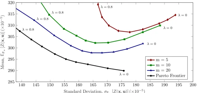
conducted for m = 5, 10, 20, and the resulting mean-risk trade space is plotted in Figure 3. The first thing to note is that the mean-risk curves for finite m do not coincide with the Pareto frontier. When we only have access to a finite number of samples we find designs that are Pareto optimal with respect to the sample distribution; however the sample distribution is not necessarily a good approximation of the true distribution, especially for low sample sizes. If the sample distribution ˆp happens to be a good approximation for the true distribution u, then we would expect the resulting mean-risk curve to be close to the Pareto frontier. In
fact, in the limit as m! 1, we expect the sample distribution to converge to the true distribution, and thus the mean-risk curve will converge to the Pareto frontier for large m. On the other hand, for small m (O(10)) we expect that the sample distribution will be a poor approximation of the true distribution on average, and thus the mean-risk curve will be far away from the Pareto frontier. This indicates that the resulting designs perform less e↵ectively under the true distribution. This trend is clearly illustrated in Figure 3, where we see that increasing the number of samples m used to approximate the true distribution u brings the mean-risk
curve closer to the Pareto frontier.
We also observe that the shape of the mean-risk curves changes as we decrease the number of samples. For small m, we see that optimizing for the mean alone no longer gives the best mean performance. Instead, shifting some of the objective weight onto the risk objective actually results in an improvement in the mean performance objective. Although this seems counterintuitive at first, this e↵ect can be explained by the fact that designs that prioritize a lower standard deviation are more general in the sense that they exhibit more consistent performance under distributions that di↵er from the distribution for which they were optimized. To see this, consider the case where = 1, and the standard deviation of the resulting design is reduced to zero. In this case the performance of the horn is constant over the range of samples, which is likely to be
140 145 150 155 160 165 170 175 180 185 190 195 200 285 290 295 300 305 310 315 320 = 0 = 0 = 0 = 0 = 0.8 = 0.8 = 0.8 = 0.8
Standard Deviation, u[Z(x, u)] (⇥10
5) M ean , u [Z (x ,u )] (⇥ 10 5) m = 5 m = 10 m = 20 Pareto Frontier
Figure 3: Mean-risk curves generated using multi-objective optimization with varying sample size for the acoustic horn design problem.
close to the full support of the true uncertain distribution. This design will thus exhibit almost identical performance for both the sample distribution and the true distribution (and any other distribution sharing the same support as the samples). In contrast, if we only optimize for the mean it is likely that the optimization algorithm will exploit the structure of the sample distribution, and find designs that perform well in regions where the sample probability density is high, while ignoring regions where the sample probability density is low. However, if these sample probability densities are not a good representation of the true densities, then the expected performance of the design under the true distribution will be poor. In this way, the designs that optimize for mean performance only are over-fit to the sample distribution, and generalize poorly to the true distribution.
From these results, we can conclude that adding robustness in the form of a risk reduction objective helps to reduce the impact of the error incurred in estimating the true uncertainty from data. This is done by ensuring that the designs we select are able to generalize from the sample distribution to the true distribution. In the next section we present a principled method for introducing this notion of robustness into the design problem, using the mathematical framework of distributionally robust optimization.
III.
Distributionally Robust Optimization
Using a multi-objective optimization approach based on estimated probability distributions, we saw the importance of ensuring that the designs we select are able to generalize to the unknown true distribution. This naturally raises the question of whether we can take this idea a step further and employ a method that explicitly seeks such designs. In this section we investigate the distributionally robust approach, which optimizes for designs that achieve good performance on average, while requiring that this average performance be robust to deviations in the distribution of the uncertainty. Section III.A formulates the problem of finding distributionally robust designs. Section III.B discusses how to select a set of probability distributions against which to robustify the design, and finally Section III.C and III.D present efficient algorithms for solving the distributionally robust design problem.
III.A. The Distributionally Robust Design Problem
The central idea behind the distributionally robust approach is to optimize the design considering a set of possible distributions of the uncertainty,12, 25which we refer to as the ambiguity set,13and denoteP. We then
seek a design that performs well on average for all distributions within the ambiguity set. This is achieved by solving a minimax problem to optimize the worst-case expected performance within the ambiguity set. This can be written mathematically as
min
x2Xmax2P [Z(x, u)] . (6)
Note that in contrast with the multi-objective approach, we are not explicitly optimizing for a reduction in the standard deviation of performance. Instead, we are optimizing only for mean performance. By using the worst-case within the ambiguity set we are adding a requirement that this mean performance must be robust to departures in the distribution of uncertainty away from the sample distribution. The inner maximization in this minimax statement involves finding the worst-case expectation over all distributions in the ambiguity set. The outer minimization finds the design that improves this worst-case expectation as much as possible. Since our model of the acoustic horn, Z(x, u), is a black-box function, we are unable to compute expectations under continuous probability distributions. Consequently, we must limit our ambiguity set to discrete approximations of these distributions. In this case the problem becomes
min x2Xmaxp2P m X i=1 piZ(x, ui). (7)
This problem is tractable, since we are able to evaluate the horn performance at the discrete support values of p, namely ui, and weight them by their corresponding probabilities pito compute the expectation.
III.B. Selecting the Ambiguity Set
The success of the distributionally robust approach relies on a careful selection of the ambiguity setP. The size ofP roughly determines the degree of conservatism of the design. On one end of the spectrum, we could limit the ambiguity set to contain only a single probability distribution, namely the sample distribution ˆ
p generated using our known data. This would reduce the problem to a traditional optimization under uncertainty for the mean, and would therefore generate the same solution as Eq. (5) with the standard deviation weight ( ) set to zero. In this case we would naturally see the same issue as in the multi-objective setting, whereby the optimization will over-fit the design to features of the sample distribution, and the resulting design will likely not generalize well to the true distribution.
On the other hand, using a large ambiguity set forces the optimization to accommodate a large range of distributions. This can ensure that the true distribution is within the ambiguity set with high probability, avoiding the problem of over-fitting and ensuring that our design will generalize. However, since the true distribution is unknown we will necessarily have to include in our ambiguity set all distributions which are plausible candidates for the true distribution. If we allow the ambiguity set to become too large, the optimization is forced to accommodate a variety of di↵erent distributions. This prevents the optimization from being able to exploit any structure in the true distribution, and will lead to poor mean performance. This can be seen if we consider expanding our ambiguity set to include every possible distribution. This gives rise to the usual worst-case optimization problem. In this situation, the worst-case distribution will always be one in which all the probability density is assigned to the worst possible realization of the uncertainty. In almost all real situations this is an unrealistic candidate for the true distribution, and so the worst-case approach leads to an overly conservative design with poor average performance. Clearly there is a trade o↵ to be made in selecting the ambiguity set. We would like the set to have a large likelihood of containing the true distribution, while avoiding the over-conservatism introduced by making the set too large.
A good ambiguity set then, is one that contains the true distribution with maximum probability for a given set size. This can be achieved by adding distributions to the ambiguity set preferentially in order of how plausible they are given our data on the uncertainty. In our case, this means we add distributions to the ambiguity set based on how similar they are to our sample distribution. To do this, we need a metric for comparing a candidate distribution p to the sample distribution ˆp. We use the L2 norm, defined by
kˆp pk2= v u u tXm i=1 (ˆpi pi)2. (8)
We then define our ambiguity set as the set of all distributions within a given L2 distance of the sample distribution. This distance is termed the radius of ambiguity and denoted r. Thus the L2 norm ambiguity set is defined by
PL2( ˆp, r ) ={ p : kˆp pk2 r } . (9)
III.C. Solving the Inner Problem
The inner maximization in Eq. (7) involves finding the distribution within the ambiguity set that generates the worst possible expected performance of our design. Given a design x, a set of samples ui, i = 1, ..., m,
and an L2 radius of ambiguity r, this can be formulated as max p m X i=1 piZ(x, ui) (10) subject to kˆp pk2 r.
Much of the appeal of using an ambiguity set defined by the L2 norm is that this problem can be solved in closed-form using Algorithm 2 below. This algorithm was originally derived in Ref. 26, for the limited case where ˆp = m, where denotes an appropriately sized vector of ones. The algorithm presented here is an extension applicable to a general ˆp. For details on the derivation of the original algorithm see Ref. 26. III.D. Solving the Outer Problem
The outer minimization in Eq. (7) involves finding a design that minimizes the worst case expectation computed in the inner problem (via Algorithm 2). This can be done using a subgradient descent method, similar to the one employed in the multi-objective approach (Algorithm 1). In fact, Algorithm 3 is exactly equivalent to Algorithm 1 in the case = 0, except that we replace the sample distribution ˆp with the worst case distribution p⇤ computed using Algorithm 2. Note in particular, that this means that the number of black-box model evaluations required to reach an optimal design is the same for the distributionally robust approach as the multi-objective approach. Since the inner problem has a closed-form solution with negligible run-time, this means the two approaches have very similar computational cost. Note that considerations about the step size ↵ and the convergence criterion used are the same as those described in Section II for Algorithm 1.
input : Discrete reference distribution ˆp,
function values at distribution support Z(x, ui)⌘ Zi ,
radius of L2 ambiguity set r.
output : Worst-case discrete distribution p⇤, on the same support as ˆp.
1 m = length(ˆp) 2 K ={1, 2, ..., m} 3 while|K| > 1 do 4 k = m |K| 5 Z =¯ 1 (m k) P i2K Zi 6 s = s 1 (m k) P i2K (Z2 i Z¯2) 7 if k = 0 then 8 pi= ˆpi+ Zi Z¯ p m s r 9 else 10 pi= 8 > < > : 0 i /2 K, ˆ pi+ 1 (m k) P i /2K ˆ pi+ r (m k)(r2 P i /2K ˆ p2 i) ( P i /2K ˆ p)2Zi Z¯ s ! i2 K. 11 end 12 if pi 0 8i 2 K then 13 p⇤= p 14 return p⇤ 15 else
16 Find critical j2 K. This is the last index of pi< 0 to become positive as we decrease r.
This can be done by analyzing the formula for piabove, i.e. setting pi= 0 and solving
for r. 17 Set K = K\ {j}. 18 end 19 end 20 pi= ( 0 i /2 K, 1 i2 K. 21 p⇤= p 22 return p⇤
input : m samples of the uncertain variables ui,
black box horn model hZ(x, ui),@Z(x,u@x i)
i
= runHornModel (x, ui),
an initial design x0.
output : Optimal Design x⇤, which solves Eq. (7) 1 x = x0, j = 0 2 repeat 3 for i = 1 to m do 4 Z(x, ui), @Z(x, ui) @x runHornModel(x, ui) 5 end
6 p⇤ computeWorstCaseP(Z(x, ui),P) ; // Solve Eq. (10), see Sec. III.C 7 G m P i=1 p⇤ i @Z(x, ui) @x 8 x x ↵(j)G 9 j = j + 1 10 until Converged ; 11 x⇤= x 12 return x⇤
Algorithm 3: Distributionally robust optimization using a black-box system model.
IV.
Results: Performance of the Distributionally Robust Approach Under
Partial Observability
To allow for a fair comparison, the experimental method used to evaluate the performance of the DRO approach is almost identical to that used for the multi-objective approach, outlined in Section II.C. The di↵erence is that now instead of the parameter , we have the analogous parameter r, the radius of ambiguity. Both of these parameters control the degree of robustness we enforce in our solution. Note however, that the maximum permissible value of r is not necessarily 1. Instead, rmaxis defined as the radius of ambiguity at
which our ambiguity set contains all possible distributions. In our case, since ˆp = m, this can be computed as the L2 norm between a uniform distribution and a degenerate distribution centered at any point on the discrete support, e.g., pi= 1 for i = 1, and 0 otherwise. This gives the closed form expression
rmax= v u u t✓1 m 1 ◆2 + m X i=2 ✓ 1 m ◆2 = r 1 1 m. (11)
Since rmaxdepends on m, we define a normalized radius of ambiguity ¯r = r/rmax, so that ¯r2 [0, 1] for any
m. For these experiments, we compute distributionally robust designs using 21 equally spaced values of ¯r. This process was repeated for 50 trials, using the same sample draws as those used for the multi-objective approach. In this way, exactly the same data and practically identical computational budget are used for both the multi-objective and distributionally robust approaches, allowing for a fair comparison between the resulting designs.
The experiments described above were carried out with m = 20 samples. The resulting average mean-risk curve for the distributionally robust approach is plotted in Figure 4, along with the analogous mean-risk curve generated using the standard multi-objective approach. We see that the DRO and MOO curves coincide at the points corresponding to ¯r = 0 and = 0 respectively. In both methods, this is the point at which zero importance is placed on robustness, and we simply optimize the sample average performance directly. The methods di↵er in the way in which robustness is introduced into the objective function, and this is manifested in the way the curves diverge for values of r and greater than zero.
It is interesting to observe that the mean-risk curve for the DRO approach has a significantly di↵erent shape to the MOO equivalent, particularly in the way that the curve doubles back on itself after the point ¯
r = 0.7. A consequence of this is that the DRO approach is unable to achieve levels of risk as low as the MOO approach. This can be explained by the fact that our objective in the DRO approach does not explicitly seek
140 145 150 155 160 165 170 175 180 185 190 195 285 290 295 300 305 310 ¯ r = 0 ¯ r = 0.7 ¯ r = 1
Standard Deviation, u[Z(x, u)] (⇥10
5) M ean , u [Z (x ,u )] (⇥ 10 5) DRO MOO Pareto Frontier
Figure 4: Mean-risk curves for the distributionally robust optimization approach with m = 20 samples, compared with the analogous mean-risk curve generated with a multi-objective approach.
to minimize the standard deviation in performance. In terms of mean performance however, we see the DRO approach outperforms the MOO approach for the entire range of risk levels attained. This is evidenced by the fact that the DRO mean-risk curve is below the MOO mean-risk curve, and therefore closer to the Pareto frontier, all the way up until the point ¯r = 0.7. This is a significant improvement, as it means that given exactly the same samples and practically equivalent computational budget, the DRO approach is able to uncover designs that perform better on average, for a given risk level.
To observe this concretely, we assume a scenario in which the designer wishes to impose a constraint that the risk level in the design must be no greater than u = 160⇥ 10
5. We thus wish to find a design that
has optimal mean performance for a risk level no greater than this value. The mean-risk trade space for this problem is shown in Figure 5. We see that the Pareto optimal design in this case, which would only be
140 145 150 155 160 165 170 175 180 185 190 195 285 290 295 300 305 310 Risk Requirement: < 160⇥ 10 5
Standard Deviation, u[Z(x, u)] (⇥10
5) M ean , u [Z (x ,u )] (⇥ 10 5) DRO MOO Pareto Frontier
Figure 5: Mean-risk trade space for m = 20 samples, in the scenario where we require the risk level to be no greater than u = 160⇥ 10
5.
of 293.5⇥ 10 5. If the designer has access to only m = 20 samples from this distribution, and they use
the standard multi-objective approach, they would expect to obtain a design with a mean performance of 299.3⇥ 10 5. This is an optimality gap of 5.8⇥ 10 5due to the fact that we only have partial observability
over the underlying distribution. If the designer instead uses our distributionally robust approach, they would obtain a design with a mean performance of 297.6⇥ 10 5. This gives an optimality gap of only 4.1⇥ 10 5, or
a reduction in the optimality gap of 29.3%.
140 145 150 155 160 165 170 175 180 185 190 195 285 290 295 300 305 310 Mean Requrement: < 298⇥ 10 5
Standard Deviation, u[Z(x, u)] (⇥10
5) M ean , u [Z (x ,u )] (⇥ 10 5) DRO MOO Pareto Frontier
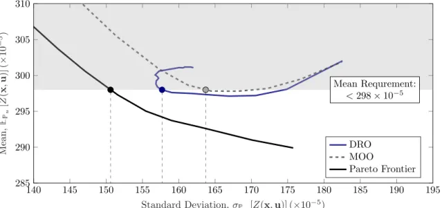
Figure 6: Mean-risk trade space for m = 20 samples, in the scenario where we require the mean performance to be no greater than 298⇥ 10 5.
We also pose an alternative scenario, in which the designer requires that the mean performance is at most 298⇥ 10 5, and wishes to find a design with minimum risk subject to this constraint. The mean-risk trade
space for this scenario is shown in Figure 6. We see that the minimum risk attainable under full observability is 150.6⇥ 10 5, while the DRO and multi-objective approaches achieve designs with risk levels of 157.7⇥ 10 5,
and 163.7⇥ 10 5respectively. This corresponds to achieving a reduction in the optimality gap of 45.8% by
using the DRO approach.
These results show that the distributionally robust approach is able to extract more useful information from the samples, and uncover designs that are not attainable using a multi-objective approach when given the same data. It also shows that the designs obtained from the distributionally robust approach can significantly outperform those found using a multi-objective approach.
145 150 155 160 165 170 175 180 185 190 195 200 285 290 295 300 305 310 315 ¯ r = 0 ¯ r = 0 ¯ r = 0 ¯ r = 1 ¯ r = 1 ¯ r = 1
Standard Deviation, u[Z(x, u)] (⇥10
5) M ean , u [Z (x ,u )] (⇥ 10 5) m = 5 m = 10 m = 20 Pareto Frontier
Figure 7: Mean-risk trade space for the distributionally robust optimization experiments
The distributionally robust optimization experiment was repeated for sample sizes m = 5 and m = 10. The results are given in Figure 7. We see that the trends observed in the m = 20 case generally carry over into the smaller sample sizes. However, as the sample size is reduced, it appears to require a higher value of ¯r before the DRO approach begins to outperform the multi-objective approach.
V.
Conclusions and Future Work
This paper has shown the potential benefits of a distributionally robust approach over a multi-objective approach for design under uncertainty. Although the distributionally robust approach in this paper has been demonstrated on a single problem, the formulation and algorithms make no assumptions about the system in question. The approach is therefore applicable to a wide range of design problems. The e↵ects of uncertainty on the quantity of interest vary depending on the system in question. Planned future work involves testing the distributionally robust approach on additional design problems, to explore whether certain characteristics of the system of interest or of the uncertainty influence the performance of the method.
There is also room for future improvements to the distributionally robust approach itself, namely, the exploration of di↵erent formulations of the ambiguity set. In this paper the ambiguity set is generated using an L2 norm. Promising alternatives used in the literature include ambiguity sets based on the Kullback-Leibler divergence,16 the Wasserstein distance,27 or moment constraints on the distributions.12 Future work will
involve exploring these alternatives in the design under uncertainty setting.
Acknowledgements
This work was supported in part by AFOSR grant FA9550-16-1-0108 under the Dynamic Data Driven Application Systems Program, by the Defense Advanced Research Projects Agency [EQUiPS program, award W911NF-15-2-0121, Program Manager F. Fahroo] and by a New Zealand Marsden Fund grant under contract UOA1520.
References
1Kennedy, M. C. and O’Hagan, A., “Bayesian Calibration of Computer Models,” Journal of the Royal Statistical Society:
Series B (Statistical Methodology), Vol. 63, No. 3, 2001, pp. 425–464.
2Beyer, H.-G. and Sendho↵, B., “Robust Optimization–A Comprehensive Survey,” Computer Methods in Applied Mechanics
and Engineering, Vol. 196, No. 33, 2007, pp. 3190–3218.
3Du, X. and Chen, W., “Efficient Uncertainty Analysis Methods for Multidisciplinary Robust Design,” AIAA journal,
4Du, X. and Chen, W., “Methodology for Managing the E↵ect of Uncertainty in Simulation-Based Design,” AIAA Journal,
Vol. 38, No. 8, 2000, pp. 1471–1478.
5Keane, A. and Nair, P., Computational Approaches for Aerospace Design: The Pursuit of Excellence, John Wiley & Sons,
2005.
6Helton, J. C., Johnson, J. D., and Oberkampf, W. L., “An Exploration of Alternative Approaches to the Representation
of Uncertainty in Model Predictions,” Reliability Engineering & System Safety, Vol. 85, No. 1, 2004, pp. 39–71.
7Rao, S. and Cao, L., “Optimum Design of Mechanical Systems Involving Interval Parameters,” Transactions-American
Society of Mechanical Engineers Journal of Mechanical Design, Vol. 124, No. 3, 2002, pp. 465–472.
8Ben-Tal, A., El Ghaoui, L., and Nemirovski, A., Robust Optimization, Princeton University Press, 2009.
9Zaman, K., Rangavajhala, S., McDonald, M. P., and Mahadevan, S., “A Probabilistic Approach for Representation of
Interval Uncertainty,” Reliability Engineering & System Safety, Vol. 96, No. 1, 2011, pp. 117–130.
10Smets, P., “Probability, Possibility, Belief: Which and Where?” Quantified Representation of Uncertainty and Imprecision,
Springer, 1998, pp. 1–24.
11Goh, J. and Sim, M., “Distributionally Robust Optimization and its Tractable Approximations,” Operations Research,
Vol. 58, No. 4-part-1, 2010, pp. 902–917.
12Delage, E. and Ye, Y., “Distributionally Robust Optimization Under Moment Uncertainty with Application to Data-Driven
Problems,” Operations research, Vol. 58, No. 3, 2010, pp. 595–612.
13Wiesemann, W., Kuhn, D., and Sim, M., “Distributionally Robust Convex Optimization,” Operations Research, Vol. 62,
No. 6, 2014, pp. 1358–1376.
14Ben-Tal, A., Den Hertog, D., De Waegenaere, A., Melenberg, B., and Rennen, G., “Robust Solutions of Optimization
Problems A↵ected by Uncertain Probabilities,” Management Science, Vol. 59, No. 2, 2013, pp. 341–357.
15Van Parys, B. P., Esfahani, P. M., and Kuhn, D., “From Data to Decisions: Distributionally Robust Optimization is
Optimal,” arXiv preprint arXiv:1704.04118 , 2017.
16Hu, Z. and Hong, L. J., “Kullback-Leibler Divergence Constrained Distributionally Robust Optimization,” Optimization
Online, 2013.
17Ng, L. W. and Willcox, K. E., “Multifidelity Approaches for Optimization Under Uncertainty,” International Journal for
Numerical Methods in Engineering, Vol. 100, No. 10, 2014, pp. 746–772.
18Ng, L. W., Huynh, D. P., and Willcox, K., “Multifidelity Uncertainty Propagation for Optimization Under Uncertainty,”
12th AIAA Aviation Technology, Integration, and Operations (ATIO) Conference and 14th AIAA/ISSMO Multidisciplinary Analysis and Optimization Conference, 2012, p. 5602.
19Marler, R. T. and Arora, J. S., “Survey of Multi-Objective Optimization Methods for Engineering,” Structural and
Multidisciplinary Optimization, Vol. 26, No. 6, 2004, pp. 369–395.
20Park, G.-J., Lee, T.-H., Lee, K. H., and Hwang, K.-H., “Robust Design: An Overview,” AIAA J , Vol. 44, No. 1, 2006,
pp. 181–191.
21Padulo, M., Campobasso, M. S., and Guenov, M. D., “Novel Uncertainty Propagation Method for Robust Aerodynamic
Design,” AIAA journal, Vol. 49, No. 3, 2011, pp. 530–543.
22Zaman, K., McDonald, M., Mahadevan, S., and Green, L., “Robustness-Based Design Optimization under Data Uncertainty,”
Structural and Multidisciplinary Optimization, Vol. 44, No. 2, 2011, pp. 183–197.
23Lee, S. W. and Kwon, O. J., “Robust Airfoil Shape Optimization Using Design for Six Sigma,” Journal of aircraft, Vol. 43,
No. 3, 2006, pp. 843–846.
24Boyd, S., Xiao, L., and Mutapcic, A., “Subgradient methods,” Lecture notes of EE392o, Stanford University, Autumn
Quarter , Vol. 2004, 2003.
25Xu, H., Caramanis, C., and Mannor, S., “A Distributional Interpretation of Robust Optimization,” Mathematics of
Operations Research, Vol. 37, No. 1, 2012, pp. 95–110.
26Philpott, A., de Matos, V., and Kapelevich, L., “Distributionally Robust SDDP,” Preprint available at
http://www.epoc.org.nz/papers/DROPaperv52.pdf .
27Esfahani, P. M. and Kuhn, D., “Data-Driven Distributionally Robust Optimization using the Wasserstein Metric: