Delayed North Atlantic Response to Solar Forcing of the Stratospheric Polar Vortex

(1)

HAL Id: insu-01576591

https://hal-insu.archives-ouvertes.fr/insu-01576591

Submitted on 23 Aug 2017

HAL is a multi-disciplinary open access

archive for the deposit and dissemination of

sci-entific research documents, whether they are

pub-lished or not. The documents may come from

teaching and research institutions in France or

abroad, or from public or private research centers.

L’archive ouverte pluridisciplinaire HAL, est

destinée au dépôt et à la diffusion de documents

scientifiques de niveau recherche, publiés ou non,

émanant des établissements d’enseignement et de

recherche français ou étrangers, des laboratoires

publics ou privés.

Seiji Yukimoto, Kunihiko Kodera, Rémi Thiéblemont

To cite this version:

Seiji Yukimoto, Kunihiko Kodera, Rémi Thiéblemont. Delayed North Atlantic Response to Solar

Forcing of the Stratospheric Polar Vortex . SOLA, Meteorological Society of Japan, 2017, 13,

pp.53-58. �insu-01576591�

(2)

Abstract

A delayed response of the winter North Atlantic oscillation (NAO) to the 11-year solar cycle has been observed and modeled in recent studies. However, the mechanisms creating this 2−4-year delay to the solar cycle have still not been well-understood. This study examines the effects of the 11-year solar cycle and the resulting modulation in the strength of the winter stratospheric polar vortex. A coupled atmosphere–ocean general circulation model is used to simulate these effects by introducing a mechanis-tic forcing in the stratosphere. The intensified stratospheric polar vortex is shown to induce positive and negative ocean temperature anomalies in the North Atlantic Ocean. The positive ocean tem-perature anomaly migrated northward and was amplified when it approached an oceanic frontal zone approximately 3 years after the forcing became maximum. This delayed ocean response is similar to that observed. The result of this study supports a previ-ous hypothesis that suggests that the 11-year solar cycle signals on the Earth’s surface are produced through a downward penetration of the changes in the stratospheric circulation. Furthermore, the spatial structure of the signal is modulated by its interaction with the ocean circulation.

(Citation: Yukimoto, S., K. Kodera, and R. Thiéblemont, 2017: Delayed North Atlantic response to solar forcing of the stratospheric polar vortex. SOLA, 13, 53−58, doi:10.2151/sola. 2017-010.)

1. Introduction

The importance of the North Atlantic oscillation (NAO) for the European weather and climate conditions has been known for a long time (Walker and Bliss 1932; van Loon and Rogers 1978; Hurrell et al. 2003). NAO is the dominant intrinsic mode of atmospheric variability over the Atlantic sector (Hurrell and Deser 2009). It is often characterized by a north–south seesaw in the sea-level pressure (SLP) between the Iceland and Azores regions. Hence, it is crucial to quantify the extent to which external drivers such as tropical sea surface temperature (SST) (Brönnimann et al. 2007) and stratospheric circulation (Kidston et al. 2015) can modulate the variability of the NAO. The role of extratropical oceans in producing interannual variations in the NAO has been pointed out (Rodwell et al. 1999; Czaja and Frankignoul 2001). The impacts of the external forcing from the 11-year solar cycle on the NAO, such as the modulation of its spatial structure (Kodera 2002) and the increase in its predictability (Dunstone et al. 2016), have also been suggested. In recent studies using long-term histor-ical data, a significant delayed response of the NAO to the 11-year solar cycle has been reported (Gray et al. 2013, 2016).

To explain this delayed response, Scaife et al. (2013) pre-sented a simple mechanistic model that treated the ocean as a heat reservoir. It was suggested that the extended memory of the ocean heat-content anomalies and their subsequent interaction with the atmosphere may produce the delayed response observed for the

NAO. Recently, the delayed solar response of the North Atlantic has also been simulated using middle-atmosphere climate system models coupled with a dynamic ocean model and an atmospheric chemistry model (Andrews et al. 2015; Thiéblemont et al. 2015). In these model simulations, the response in the Atlantic sector related to the solar forcing was found to be delayed by approx-imately 3 years, which is similar to the observed response. This suggests that the delayed response is related to the atmosphere– ocean response.

For the above-mentioned simulations, fluctuations in the total solar irradiance and the solar spectrum (from infrared to ultravio-let (UV)) were considered. Hence, the top-down influence induced by the solar UV-heating changes in the stratosphere (Andrews et al. 2015; Thiéblemont et al. 2015) cannot be easily separated from the bottom-up influence (e.g., Meehl et al. 2009) initiated by a direct heating of the Earth’s surface. To focus solely on the role of stratospheric circulation changes, an idealized simulation was conducted by directly applying accelerating stratospheric zonal winds to a CGCM (Yukimoto and Kodera 2007). This demon-strated that the characteristic features of the global distribution of the solar signal in the Earth’s surface temperature can be realized by forcing in the stratospheric zonal winds (Kodera et al. 2016). The forcing in Kodera et al. (2016) had only seasonal variation and did not include any quasi-decadal variation. To investigate the cause of the delayed response of the NAO, a similar CGCM simulation was conducted in this study with the exception that the zonal wind forcing was modulated with the 11-year cycle.

This study describes the model used and the simulations applied to this model in Section 2; the simulation results for the tropospheric circulation and the ocean temperatures are presented in Section 3; and a brief discussion and conclusion from these results is presented in Section 4.

2. Model and experiment

The Meteorological Research Institute (MRI) CGCM (MRI-CGCM2.3) (Yukimoto et al. 2006) is used for this experiment. The atmospheric model has a T42 spectral horizontal resolution and 30 vertical levels with the top level at 0.4 hPa. The ocean model has a 2.5° longitude and 2.0° latitude horizontal resolution, except for a 0.5° latitude resolution near the equator, with 23 vertical layers.

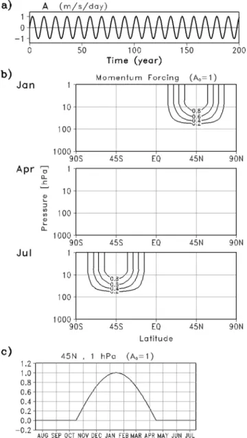
In this simulation, stratospheric zonal winds are forced by adding the zonal angular momentum in the winter stratosphere at levels above 100 hPa. The momentum forcing (Fm) is essentially the same as that used in Yukimoto and Kodera (2007) with the exception that the amplitude (A) of the forcing varies with the 11-year cycle and is expressed as,

A = A0 sin (2π t/11-year), (1)

where A0 = 1 m s−1/day, and t denotes the time (years). It should

be noted that the forcing is applied only in the winter hemisphere as follows.

Fm = A f (p)(sin 2ϕ)2_{MAX{0, cos [2π(n − n}

0)/365]}, (2)

where n denotes the day of the year and n0 denotes the central day

of the winter (15 January in the Northern Hemisphere (NH) and 15 July in the Southern Hemisphere (SH)). The vertical profile f (p) is expressed as follows:

Delayed North Atlantic Response to Solar Forcing

of the Stratospheric Polar Vortex

Seiji Yukimoto

1

_{, Kunihiko Kodera}

2

_{, and Rémi Thiéblemont}

3 1

_{Meteorological Research Institute, Tsukuba, Japan}

2

_{Institute for Space-Earth Environmental Research, Nagoya University, Nagoya, Japan}

3

_{Laboratoire Atmosphères Milieux Observations Spatiales, Guyancourt, France}

(3)

winter–spring that are associated with the 11-year cycle momen-tum forcing. Stronger zonal-mean zonal winds were induced by the forcing in the winter stratosphere. The magnitude of the zonal wind anomalies is comparable with that observed (Kodera and Kuroda 2002), implying that the magnitude of the momentum forcing is fairly realistic. The simulation shows that the signal penetrates into the troposphere from late winter to spring, which is similar to the polar night jet oscillation through the interaction between mean-flow and planetary waves and transient eddies (Kuroda and Kodera 1999). A warming of ~1 K in the tropical lower troposphere is also simulated (not shown), which implies the top-down propagation of the signal via the tropics (Simpson et al. 2009) as another pathway to the tropospheric response.

The response of the SLP (Fig. 2 bottom) first occurs in the polar region in January. Following this, high pressure develops over the surrounding oceans, i.e., the Atlantic and the Pacific, during late winter–spring. The change in the SLP in the mid-latitudes occurs in association with an increased equatorward propagation of tropospheric eddies (see E-P flux in Fig. 2) and the development of easterly anomalies in the subtropics. Such a seesaw pattern in the surface pressure between the polar and sur-rounding regions is termed as Arctic Oscillation (AO) or surface annular mode (Thompson and Wallace 2000). It should be noted that in spite of the nomenclature (Gerber and Thompson 2016), surface annular mode in the NH includes a fairly large stationary wave component; the polar vortex is shifted toward eastern Canada in the positive phase, which advects polar cold air to the northeast coast of American continent (see Fig. 11 in Thompson and Wallace 2000).

The earlier section describes the way in which changes induced by the momentum forcing in the stratosphere can pene-trate into the troposphere during the winter–spring. The delayed response to the stratospheric forcing by means of a lagged regression is explained in this section. Regressed zonal-mean zonal winds and SLPs in February–March are shown for lags of −2, 0, and +2 years (Fig. 3). The zonal-mean zonal wind response is naturally the largest at a 0-year lag, but a seesaw pattern of the zonal-mean zonal wind anomalies between the subtropics and subpolar region persists until a +2-year lag in the troposphere. It was also noticed that the center of the positive anomalous zonal winds near the surface moves northward with time from 45°N at a −2-year lag to 55°N at a +2-year lag. This seesaw pattern of zonal winds at a 0-year lag is related to the formation of a seesaw pattern of the SLP in the North Atlantic sector between the Iceland and Azores regions, i.e., the NAO. The SLP response at a 0-year lag is accompanied by a positive anomaly in the North Pacific that constitutes the annular pattern known as AO. The negative SLP anomaly declines at a +2-year lag, although it is still significant near Greenland (Fig. 3). The simulated SLP response shows no sign of a time lag but peaks at 0-year lag. This is inconsistent with the analysis of SLP reconstruction by Gray et al. (2013) which shows a peak of positive NAO-like response in 2−3 years after the solar max.

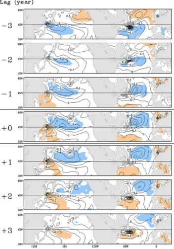
Lagged regressions of the SST for the 11-year-cycle forcing are displayed in Fig. 4 for approximately half of an 11-year cycle from −3 to +3-year lags. As the forcing is a purely periodic function, the response calculated by the linear regression is also periodic. A significant response in the SST exists throughout the cycle in the Atlantic sector. A cold anomaly appears near the western coast of the Atlantic around 40°N−45°N at a −3-year lag, which moves northeastward with time. Unlike the SLP response, the largest positive and negative anomalies of 0.9 K and −1.1 K, respectively, are found between 40°N and 45°N at a lag of +3 and −3 years, respectively. In contrast, in the Pacific sector, the largest SST anomalies are produced near the coastal region at a 0-year lag. The delayed response in the Pacific sector shows no amplification; the negative anomalies extend eastward from the northwestern Pacific but their amplitude decreases with time.

Figure 5 compares the present model result with the observed lagged solar response for SSTs. The observed solar signal is obtained from the solar component of a multiple linear regression (MLR) of winter (December–February)-mean SSTs of the

histori-f (p) = 1 p < 10

= ln(p/100)/ln(0.1) 10 < p < 100

= 0 p > 100, (3)

where p denotes the pressure (hPa) and ϕ denotes the latitude (radians). The time series of the amplitude A and the spatial struc-ture of Fm in January, April, and July are shown in Figs. 1a and 1b, respectively. The seasonal evolution of Fm at 45°N and p = 1 hPa is shown in Fig. 1c.

The model is integrated 200 years each with and without the momentum forcing for the ‘forced’ and ‘control’ simulations, respectively.

3. Results

The response to the stratospheric forcing was investigated through a regression of the variables for the amplitude, A, of the 11-year cycle momentum forcing. First, the seasonal features of the simultaneous response were examined. The top panels in Fig. 2 indicate the zonal-mean zonal wind anomalies during the boreal

Fig. 1. (a) A time series of the amplitude of momentum forcing, A, in eq. (1), (b) the spatial structure of the momentum forcing in January, April, and July, from top to bottom, respectively, and (c) seasonal evolution of the momentum forcing at 45°N and p = 1 hPa.

(4)

cal Hadley Center Sea Ice and Sea Surface Temperature (HadISST) data set for the period from 1870 to 2010. The MLR method is useful for separating the influence of multiple external forcing variables (e.g., anthropogenic, volcanic, and solar forcing) on the observed SST variability. We used the same MLR and explanatory variables (i.e., CO2 concentration, Niño3.4 index, F10.7 cm solar

radio flux index, global aerosol optical depth at 550 nm, and two orthogonal QBO indices) as in Kodera et al. (2016). Northward shift of a pair of positive and negative anomalies were clearly seen in both simulated and observed responses. The northward shift further extends from the midlatitudes to the Norwegian Sea. The amplitude of the positive anomalies increases when they approach the oceanic frontal zone (40°N−45°N) at a +2-year lag. At a +3-year lag, new negative anomalies are produced in the tropics forming a tri-pole pattern, a characteristic feature of the SST

asso-ciated with the NAO. The northward shift of the anomalous SSTs suggests that treating the ocean as a simple passive heat reservoir (Scaife et al. 2013) to explain the response to the quasi-decadal stratospheric forcing is not sufficient and the transport processes also need to be considered.

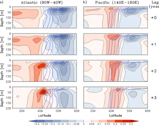
Lagged responses of the upper ocean temperature zonally averaged for the Atlantic sector (80°W−40°W) and the Pacific sector (140°E−180°E) are displayed in Fig. 6. In the Atlantic sector, a positive signal at approximately 50 m depth initiated by the winter mixed-layer is preserved beneath the shallow summer mixed-layer (~20 m depth). The signal at depth migrates north-ward and amplifies as it approaches to the ocean frontal zone at +2-year to +3-year lags. The propagation speed roughly agrees with the observed speed in SST anomalies of 2−3 cm s−1_for

decadal NAO variability (Visbeck et al. 2003). Outcropping of the

Fig. 2. Monthly mean (November, January, and March, from left to right) (top) zonal-mean zonal wind (contours) , E–P flux (vectors) and (bottom) SLP in the NH regressed for the 11-year cycle forcing. The regions exceeding a significance level of 95% are shaded. Blue and red colors indicate negative and positive values, respectively.

Fig. 3. Lagged regression with 11-year cycle forcing. The top and bottom panels represent the February–March zonal-mean zonal wind and SLP, respec-tively. From left to right, there is a lag of −2, 0 and +2 years.

(5)

signal due to a deep mixing in the following winters (not shown) leads to the SST anomaly that can interact with the atmosphere. In the Pacific sector, on the other hand, a positive anomaly initially located in the ocean frontal zone exhibits little amplification with time.

Next, the way in which coupling with the ocean modulates the tropospheric circulation variability is described. Figure 7 shows the power spectra of AO indices from different simulation runs. The red line indicates a run of the atmospheric general circula-tion model (AGCM) with climatological SSTs taken from the control simulation of the CGCM, whereas the black line is for the control simulation of the CGCM. Length of the CGCM control and AGCM simulations are 100 years and 30 years, respectively. When the atmosphere is not coupled with the ocean, the spectrum of the AO shows no variation with timescale, suggesting a white noise-like process. In contrast, including the ocean coupling enhances low frequency variations, leading to a reddening of the spectrum. When the 11-year cycle forcing is added to the CGCM (green line), a large 11-year peak appears.

4. Discussion and concluding remarks

The impact of the winter stratospheric polar vortex on the oceans for quasi-decadal timescales was studied by adding an 11-year momentum forcing to the winter stratosphere of the CGCM.

For the troposphere, the response lagged the forcing by 1−2 months and was maximized in late winter–spring, whereas a longer lagged response was found in the ocean. However, the sim-ulated atmospheric response does not show a longer delay unlike the observed SLP response that peaks 2−3 years after the solar max. The model probably has too weak atmospheric responses to the SST anomalies as suggested by Scaife et al. (2013). It is implied that the atmospheric perturbation is dominated by direct response to the stratospheric forcing rather than feedback from the ocean response.

Northward migration of a pair of positive and negative anomalies was simulated throughout the 11-year cycle in the North Atlantic Ocean. The amplification of these anomalous SSTs

Fig. 4. Lagged regression with 11-year cycle forcing. Each panel rep-resents the February–April mean SST. From top to bottom, there is a lag of −3, −2, −1, 0, +1, +2, and +3 years, respectively. The contour interval is 0.1 K.

Fig. 5. (a) Lagged regression with 11-year cycle forcing for December–February mean SSTs in the simulation. The isothermal lines represent the climato-logical SSTs around the frontal region (thick blue contours). (b) Solar component of the observed December–February mean SSTs extracted from a lagged multiple regression for the time period of 1880−2010. The contour interval is 0.05K. From left to right, there is a lag of 0, 1, 2, and 3 years, respectively.

(6)

occurred when the upper ocean temperature anomalies approached the ocean frontal zone. Anomalous SST fields transform to NAO-like pattern approximately 3 years after the maximum of the forcing, similar to the observed solar signal for the Atlantic SSTs. The present stratospheric forced simulation results also show that there is no apparent delay in the Pacific sector, except for some eastward extension of the decaying negative anomalous SSTs in the subpolar region.

The reemergence mechanism suggests that a deep signal, that is initiated by the winter mixed layer, persists at a depth through-out summer and reappears at the surface in the following winter. Provided that atmosphere-ocean feedback is strong enough, repeated interaction with the reemergence mechanism can explain the 2−3-year delayed response by the integrated effects as

pro-posed by Scaife et al. (2013). However, this does not fully explain the difference in lagged response between the Atlantic and Pacific sectors. The present CGCM simulation demonstrates that a longer delay in the Atlantic Ocean can arise from the migration of ocean temperature anomalies into ‘hotspot’ in the oceanic frontal zone where strong interactions occur with the atmosphere. For instance, it is known that midlatitude oceanic fronts play an important role in the interaction between the atmosphere and ocean through the modulation of transient eddies (Nakamura et al. 2004; Kwon et al. 2010). Using an aqua-planet model simulation, Nakamura et al. (2008) suggested in particular that the midlatitude oceanic fronts can enhance annular mode variability.

The question related to the absence of the delay in the Pacific sector (compared to the Atlantic) remains unanswered. One possibility discussed by Kodera et al. (2016) suggests that the AO includes a large stationary wave component. During the positive phase of the AO, warming occurs over the midlatitudes of the Eur-asian continent. However, in the Atlantic sector, the polar vortex is shifted toward the east of Canada, and the cold air moves to the midlatitudes along the east coast of the American continent. As a result, AO-related warming occurs in the subtropics in the Atlantic sector, as can be seen in Fig. 4 at a 0-year lag. This warm anomaly in the subtropical Atlantic Ocean is transported northward and arrives near the frontal zone 2−3 years later when a large ampli-fication occurs. In contrast, in the Pacific sector, the warming because of the positive phase of the AO is initially produced near the ocean frontal zone. Therefore, the interaction occurs without delay and anomalies decay with time.

There could be an additional factor that may create a differ-ence in the response between the Atlantic and Pacific sectors. A modification of the AO spectrum owing to a non-linear interaction between the external forcing and internal variation is suggested in Fig. 7. The spectrum of the observed winter-mean NAO index is red, but it is slightly enhanced around the 8−10 year band (Hurrell et al. 2003). For the Pacific internal mode (Pacific Decadal Oscil-lation), the power is largest for the longer periods of the 15−25

Fig. 7. Power spectra of the AO indices for different runs using models with the same atmospheric component: (red lines) AGCM, (black lines) CGCM control, and (green lines) CGCM forced simulations.

Fig. 6. Lagged regression with 11-year cycle forcing for the upper ocean temperature in summer (June–August) zonally averaged for (a) the Atlantic sector (80°W−40°W) and (b) the Pacific sector (140°E−180°E). The contour interval is 0.05 K. The blue contours represent the climatological temperature be-tween 6°C and 12°C around the frontal region. From top to bottom, there is a lag of 0, +1, +2, and +3 years, respectively.

(7)

year band (Minobe 1999). As the NAO has some power near the 11-year cycle, resonance may take place more easily. In fact, the numerical simulation of Thiéblemont et al. (2015) suggested a phase locking of the NAO with the 11-year solar cycle.

The present result confirms the previous hypothesis reported by Kodera et al. (2016), which stated that the major solar influ-ence on the Earth’s surface can be produced through changes in stratospheric circulation, and the spatial structure of the solar signal at the Earth’s surface is largely conditioned by atmosphere’s interaction with the ocean.

Acknowledgements

The authors are grateful to the anonymous reviewers for their constructive comments. This work was supported in part by JSPS Grants-in-Aid for Scientific Research 22106009, (S)24224011 and (C)25340010.

Edited by: T. Hirooka

References

Andrews, M. B., J. R. Knight, and L. J. Gray, 2015: A simulated lagged response of the North Atlantic Oscillation to the solar cycle over the period 1960−2009. Environ. Res. Lett.,

10, 054022, doi:10.1088/1748-9326/10/5/054022.

Brönnimann, S., E. Xoplaki, C. Casty, A. Pauling, and J. Luter-bacher, 2007: ENSO influence on Europe during the last centuries. Climate Dyn., 28, 181−197, doi:10.1007/s00382-006-0175-z.

Czaja, A., and C. Frankignoul, 2002: Observed impact of Atlantic SST anomalies on the North Atlantic Oscillation. J. Climate,

15, 606−623.

Dunstone, N., D. Smith, A. Scaife, L. Hermanson, R. Eade, N. Robinson, M. Andrews, and J. Knight, 2016: Skilful pre-dictions of the winter North Atlantic Oscillation one year ahead. Nat. Geosci., 9, 809−815, doi:10.1038/ngeo2824. Gerber, E., and D. Thompson, 2016: What makes an annular mode

“annular”? J. Atmos. Sci., doi:10.1175/JAS-D-16-0191.1, in press.

Gray, L. J., J. Beer, M. Geller, J. D. Haigh, M. Lockwood, K. Matthes, U. Cubasch, D. Fleitmann, G. Harrison, L. Hood, J. Luterbacher, G. A. Meehl, D. Shindell, B. van Geel, and W. White, 2010: Solar influences on climate. Rev. Geophys.,

48, RG4001, doi:10.1029/2009RG000282.

Gray, L. J., A. A. Scaife, D. M. Mitchell, S. Osprey, S. Ineson, S. Hardiman, N. Butchart, J. Knight, R. Sutton, and K. Kodera, 2013: A lagged response to the 11 year solar cycle in observed winter Atlantic/European weather patterns. J.

Geophys. Res., 118, 13, 405−413, 420, doi:10.1002/2013JD

020062.

Gray, L. J., T. J. Woollings, M. Andrews, and J. Knight, 2016: Eleven-year solar cycle signal in the NAO and Atlantic/ European blocking. Quart. J. Roy. Meteor. Soc., 142, 1890− 1903, doi:10.1002/qj.2782.

Hurrell, J. W., Y. Kushnir, M. Visbeck, and G. Ottersen, 2003: The North Atlantic Oscillation, climatic significance and environmental impact: An overview of the North Atlantic Oscillation. AGU Geophysical Monograph, 134, Hurrell, J. W., Y. Kushnir, G. Ottersen, and M. Visbeck, Eds., 1−35. Hurrell, J. W., and C. Deser, 2009: North Atlantic climate

vari-ability: The role of the North Atlantic oscillation. J. Marine

Systems, 78, 28−41.

Kidston, J., A. A. Scaife, S. C. Hardiman, D. M. Mitchell, N. Butchart, M. P. Baldwin, and L. J. Gray, 2015: Stratospheric influence on tropospheric jet streams, storm tracks and surface weather. Nat. Geosci., 8, 433−440, doi:10.1038/ ngeo2424.

Kodera, K., 2002: Solar cycle modulation of the North Atlantic Oscillation: Implication in the spatial structure of the NAO.

Geophys. Res. Lett., 29, 1218, doi:10.1029/2001GL014557.

Kodera, K., R. Thiéblemont, S. Yukimoto, and K. Matthes, 2016: How can we understand the global distribution of the solar cycle signal on the Earth’s surface? Atmos. Chem. Phys., 16, 12925−12944, doi:10.5194/acp-16-12925-2016.

Kuroda, Y., and K. Kodera, 1999: Role of planetary waves in the stratosphere-troposphere coupled variability in the northern hemisphere winter. Geophys. Res. Lett., 26, 2375−2378. Kwon, Y.-O., M. A. Alexander, N. A. Bond, C. Frankignoul, H.

Nakamura, B. Qiu, and L. A. Thompson, 2010: Role of the Gulf Stream and Kuroshio–Oyashio systems in large-scale atmosphere–ocean interaction: A review. J. Climate, 23, 3249−3281.

Nakamura, H., T. Sampe, Y. Tanimoto, and A. Shimpo, 2004: Observed associations among stormtracks, jet streams and midlatitude oceanic fronts. Earth’s Climate: The Ocean–

Atmosphere Interaction, Geophys. Monogr., 147, Amer.

Geophys. Union, 329−346.

Nakamura, H., T. Sampe, A. Goto, W. Ohfuchi, and S.-P. Xie, 2008: On the importance of midlatitude oceanic frontal zones for the mean state and dominant variability in the tropospheric circulation. Geophys. Res. Lett., 35, L15709, doi:10.1029/2008GL034010.

Meehl, G. A., J. M. Arblaster, K. Matthes, F. Sassi, and H. van Loon, 2009: Amplifying the Pacific climate system response to a small 11-year solar cycle forcing. Science, 325, 1114− 1118, doi:10.1126/science.117287.

Minobe, S., 1999: Resonance in bidecadal and pentadecadal climate oscillations over the North Pacific: Role in climatic regime shifts. Geophys. Res. Lett., 26, 855−858.

Rodwell, M. J., D. P. Rowell, and C. K. Folland, 1999: Oceanic forcing of the wintertime North Atlantic Oscillation and European climate. Nature, 398, 320−323.

Scaife, A. A., S. Ineson, J. R. Knight, L. J. Gray, K. Kodera, and D. M. Smith, 2013: A mechanism for lagged North Atlantic climate response to solar variability. Geophys. Res. Lett.,

40, 434−439, doi:10.1002/grl.50099.

Simpson, I. R., M. Blackburn, and J. D. Haigh, 2009: The role of eddies in driving the tropospheric response to stratospheric heating perturbations. J. Atmos. Sci., 66, 1347−1365, doi: 10.1175/2008JAS2758.1.

Thiéblemont, R., K. Matthes, N.-E. Omrani, K. Kodera, and F. Hansen, 2015: Solar forcing synchronizes decadal North Atlantic climate variability. Nature Commun., 6, 8268, doi: 10.1038/ncomms9268.

Thompson, D. W. J., and J. M. Wallace, 2000: Annular modes in the extratropical circulation. Part I: Month-to-month vari-ability. J. Climate, 13, 1000−1016.

Van Loon, H., and J. C. Rogers, 1978: The Seesaw in winter tem-peratures between Greenland and Northern Europe. Part I: General description. Mon. Wea. Rev., 106, 296−310. Visbeck, M., E. P. Chassignet, R. G. Curry, T. L. Delworth, R. R.

Dickson, and G. Krahmann, 2003: The ocean’s response to North Atlantic Oscillation variability. The North Atlantic

Oscillation, Geophysical Monograph 134, American

Geo-physical Union, doi:10.1029/134GM06.

Walker, G. T., and E. W. Bliss, 1932: World weather V. Mem. Roy.

Meteorol. Soc., 4, 53−84.

Yukimoto, S., A. Noda, T. Uchiyama, S. Kusunoki, and A. Kitoh, 2006: Climate change of the twentieth through twenty-first centuries simulated by the MRI-CGCM2.3. Pap. Meteor.

Geophys., 56, 9−24.

Yukimoto, S., and K. Kodera, 2007: Annular modes forced from the stratosphere and interactions with the ocean. J. Meteor.

Soc. Japan, 85, 943−952.

Manuscript received 14 December 2016, accepted 22 February 2017 SOLA: https://www.jstage.jst.go.jp/browse/sola/