Numerical solutions of generalized fractional pantograph equations with variable coefficients using shifted Chebyshev polynomials

HAL Id: hal-02884254

https://hal.archives-ouvertes.fr/hal-02884254

Submitted on 4 May 2021

HAL is a multi-disciplinary open access

archive for the deposit and dissemination of

sci-entific research documents, whether they are

pub-lished or not. The documents may come from

L’archive ouverte pluridisciplinaire HAL, est

destinée au dépôt et à la diffusion de documents

scientifiques de niveau recherche, publiés ou non,

émanant des établissements d’enseignement et de

Numerical solutions of generalized fractional pantograph

equations with variable coefficients using shifted

Chebyshev polynomials

Li-Ping Wang, Yi-Ming Chen, Da-Yan Liu, Driss Boutat

To cite this version:

Li-Ping Wang, Yi-Ming Chen, Da-Yan Liu, Driss Boutat. Numerical solutions of generalized

frac-tional pantograph equations with variable coefficients using shifted Chebyshev polynomials.

In-ternational Journal of Computer Mathematics, Taylor & Francis, 2019, 96 (12), pp.2487-2510.

�10.1080/00207160.2019.1573992�. �hal-02884254�

Numerical solutions of generalized fractional

pantograph equations with variable coefficients using

shifted Chebyshev polynomials

Li-Ping Wanga_{, Yi-Ming Chen}a,b,c_{, Da-Yan Liu}d,∗_{, Driss Boutat}d

a_{College of Sciences, Yanshan University, Qinhuangdao, Hebei, P.R.China, 066004.}

b_{LE STUDIUM RESEARCH PROFESSOR, Loire Valley Institute for Advanced Studies,}

Orl´eans, France

c_{PRISME (INSA-Institut National des sciences appliqu´ees) -88, Boulvevard Lahitolle,}

18000 Bourges, France

d_{INSA Centre Val de Loire, Universit ´e d’Orl´eans, PRISME EA 4229, Bourges Cedex}

18022, France

Abstract

In this paper, an efficient numerical technique based on the shifted Chebyshev polynomials (SCPs) is established to obtain numerical solutions of generalized fractional pantograph equations with variable coefficients. These polynomials are orthogonal and have compact support on [0, L]. We use these polynomi-als to approximate the unknown function. Using the properties of the SCPs, we derive the generalized pantograph operational matrix of SCPs and the one of fractional-order differentiation. Then the original problems can be trans-formed to a system of algebraic equations based on these matrices. By solving these algebraic equations, we can obtain numerical solutions. In addition, we investigate the error analysis and introduce the process of error correction for improving the precision of numerical solutions. Lastly, by giving some examples and comparing with other existing methods, the validity and efficiency of our method is demonstrated.

Keywords: Shifted Chebyshev polynomials, Operational matrix, Generalized fractional pantograph equations, Numerical solution, Error analysis

∗_{Corresponding author}

Email address: dayan.liu@insa-cvl.fr (Da-Yan Liu)

URL: Wangliping2500@163.com (Li-Ping Wang), chenym@ysu.edu.cn (Yi-Ming Chen),

1. Introduction

Fractional calculus is a branch of calculus theory, which makes calculus theo-ry more perfect. In recent decades, fractional calculus have been widely used in various areas, such as viscoelasticity [1, 2], economics [3], control theory [4, 5], and fractals dynamics [6]. One of the interesting research topics is the design

5

of fractional differentiators [7] to compute fractional differentials of unknown signals in a noisy environment. With the application of fractional differential equations in more and more scientific fields, the study of numerical calculations of the differential equations of fractional order is particularly important. At present, the majority of scholars have studied different kind of vigorous

nu-10

merical methods to obtained an approximate solution of fractional differential equations. These methods include Chebyshev collocation method [8], Laplace transform method [9], differential transform method [10, 11], Adomian decompo-sition method [12], Legendre operational matrix [13], and CAS wavelet method [14], etc.

15

Delay differential equations have many applications in different fields, such as biological, industrial, electronic, chemical and transportation systems [15, 16, 17]. To obtain the numerical solutions of delay differential equations, Many re-searchers have studied different kind of vigorous techniques [18]. The functional differential equations with proportional delay are generally called to pantograph

20

equations or generalized pantograph equations. As the one of the most impor-tant types of delay differential equations, the pantograph equation or the gen-eralized pantograph equation can explaining various physical phenomena. And they are used in many fields. In recent years, there have been many numerical methods for solving pantograph differential equations or generalized pantograph

25

equations of integer order, such as Chebyshev polynomials [19], Bernoulli poly-nomials [20], variational iteration method [21], etc. Further, [22] introduces the stability properties of many numerical techniques for nonlinear generalized pantograph equations.

The fractional delay differential equation is a generalization of the delay

d-30

ifferential equation to arbitrary non-integer order. Fractional delay differential equations are adapted to many fields, such as hydraulic networks, automatic control, long transmission lines, economy and biology [23]. The numerical cal-culation of fractional delay differential equations has also attracted the attention of many scholars. Because the fractional delay differential equations cannot be

35

analytically solved, different numerical methods [24, 25, 26] have been devoted to obtain the approximate solutions. Sherif et al. [27] considered the Spline func-tions to solve fractional delay differential equation. Authors of [28] investigated modified Laguerre wavelets method. Modified Chebyshev wavelet methods and a operational matrix based on Bernoulli wavelets are utilized in [29, 30].

How-40

ever, there are few scholars that pay attention to study the numerical methods of fractional pantograph delay differential equations. From these works we can mention, Y Yang and Y Huang [32] have studied the existence of solutions of nonlinear fractional pantograph equations with the order of the derivative is in [0, 1]; Using spectral-collocation methods, Yang and Huang [31] obtained the

45

approximate solution for fractional pantograph delay-integro-differential equa-tions; the approximate solution of fractional pantograph differential equations can be obtained by using the explicit formula of the generalized fractional-order Bernoulli wavelet in [33].

The polynomial approximation theory is an important branch of the

func-50

tion approximation theory. As the name suggests, polynomials are used to approximate a function whose analytical form is more complex or whose an-alytical form is unknown. In general, the polynomial has many advantages, such as its structure is clear, its calculation is simple and it is relatively easy to integral and derivative. For some complex problems, applying

polynomi-55

als to approximate function , and then studying the laws of actual problems, the problems can be simplified. At present, polynomial approximation theo-ry has been widely used in different fields, such as numerical approximation theory, engineering calculation, and practical life. In this paper, based on the properties of the shifted Chebyshev polynomials, we derive SCPs generalized

pantograph operational matrix. And with the aid of the operational matrix of fractional differentiation of SCPs, generalized pantograph operational matrix of fractional-order differentiation is obtained. We combine polynomial approxima-tion theory and operaapproxima-tional matrix to solve the following generalized fracapproxima-tional pantograph equation with variable coefficients

65 c_Dβ_{u (t) = b (t) u (t) +} J ∑ j=0 r₋₁ ∑ n=0 vj,n(t)cDαnu (qj,nt− rj,n) + g (t) , 0≤ t ≤ L, (1) subject to the initial conditions

u(n)(0) = dn, n = 0, 1,· · · , r − 1, (2)

where dn, qj,nand rj,nare real or complex coefficients, r− 1 < α ≤ r, 0 < α0< α1 <· · · < αr−1 < β, while b (t), vj,n(t) and g (t) are continuous functions in

the interval [0, L] ,c_Dβ _andc_Dαn_{denote fractional derivatives in the Caputo’s}

sense.

70

The rest of the paper is organized as follows: Section 2 introduces some mathematical preliminaries of fractional calculus. In Section 3, we review the basic definitions of shifted Chebyshev polynomials and discuss the polynomial approximation theory. In Section 4, we derive the SCPs generalized pantograph operational matrix and the one of fractional-order differentiation. In Section 5,

75

we apply the proposed method to solve the generalized fractional pantograph equations. The error correction and error analysis are given in Section 6. In Section 7, the proposed approach is tested through several numerical examples. Finally, a conclusion is given in Section 8.

2. Basic definitions of fractional calculus

80

In this section, we review the necessary definitions and preliminaries of frac-tional calculus theory that will be used in this article.

Definition 1. The Riemann-Liouville fractional integral operator of f (t) is de-fined as

85 RL_Iβ_{f (t) =}        1 Γ (β) ∫ t 0 (t− T )β−1f (T ) dT, β > 0, t > 0, f (t), β = 0. (3)

The Riemann-Liouville fractional differential operator of order β is derived by the definition of the Riemann-Liouville fractional integral operator

RL Dβf (t) =        1 Γ (n− β) dn dtn ∫ t 0 f (T ) (t− T )β−n+1dT , β > 0, n− 1 ≤ β < n, dnf (t) dtn , β = n, t > 0. (4)

Definition 2. The fractional differential operator of order β in the Caputo sense is defined as 90 c_Dβ_{f (t) =}        1 Γ (n− β) ∫ t 0 f(n)(T ) (t− T )β−n+1dT , n− 1 ≤ β < n, dnf (t) dtn , β = n, t > 0. (5)

For the Caputo differential operator, we have

c Dtβt m =      0, f or m∈ N0and m <⌈β⌉ , Γ (m + 1) Γ (m + 1− β)t m−β_{, f or m∈ N} 0 and m≥ ⌈β⌉ or m /∈ N0and m >⌊β⌋ . (6) where N0={0, 1, 2, · · · }.

3. Shifted Chebyshev polynomials

95

3.1. Properties of the shifted Chebyshev polynomials

The well-known Chebyshev polynomials are defined on the interval [−1, 1], and are derived by orthogonalizing the sequence{1, t, · · · tn_{· · · }.}

The specific form of the Chebyshev polynomials can be obtained by the following recurrence relation

100

where T0(z) = 1 and T1(z) = z. To use the Chebyshev polynomials on the

extended interval [0, L], it is necessary to shift the defining domain [−1, 1]. The shifted Chebyshev polynomials on [0, L] can easily be derived by introducing the change of variables z = 2t

L − 1. We can denote the shifted Chebyshev

polynomials Ti

(_2t

L − 1

)

by HL,i(t), then HL,i(t) can be determined with the

105

aid of the following recurrence formula

HL,i+1(t) = 2 ( 2t L − 1 ) HL,i(t)− HL,i₋₁(t) , i = 1, 2,· · ·

where HL,0(t) = 1 and HL,1(t) = 2t_L − 1 . The analytical form of the shifted

Chebyshev polynomials HL,i(t) of degree i is given by

HL,i(t) = Ti ( 2t L − 1 ) = i i ∑ k=0 (−1)i−k (i + k− 1)! (2k)! (i− k)! (2)2k Lk (t) k , i = 1, 2,· · · (7) where HL,i(0) = (−1) i and HL,i(L) = 1.

The shifted Chebyshev polynomials satisfy the following orthogonality

rela-110

tion _∫

L

0

HL,j(t) HL,k(t) ωL(t) dt = hκ, (8)

where the weight function ωL(t) = √_Lt1_−t2 and hk =

   bk 2π, k = j, 0, k̸= j, b0 = 2, bk = 1, k≥ 1. 3.2. Function approximation

A function u (t)∈ L2([0, L]) can be expanded in terms of the shifted

Cheby-115

shev polynomials as follows

u (t) =

∞

∑

i=0

ciHL,i(t), (9)

where the coefficients ci are obtained by

ci= 1 hi ∫ L 0 u (t)HL,i(t) ωL(t) dt, i = 0, 1, 2,· · ·

If we consider truncated series in Eq. (9), we can get

u (t)≈

m

∑

i=0

where C = [c0, c1,· · · , cm] T , Φm(t) = [HL,0(t) , HL,1(t) ,· · · , HL,m(t)] T . (11)

4. SCPs operational matrix for solving the pantograph equations

120

In this part, we derive the necessary SCPs generalized pantograph opera-tional matrix and the fracopera-tional generalized pantograph operaopera-tional matrix .

From Eq. (7), Φm(t) can be denoted by the product of two matrices

Φm(t) = AZm(t) , (12)

where

Zm(t) = [1, t,· · · , tm]

T .

The matrix A is SCPs coefficient matrix and we assume each item of the

125

matrix A can be write as follows

A =         P0,0 0 ... 0 P1,0 P1,1 ... 0 ... ... . .. ... Pm,0 Pm,1 ... Pm,m         , (13) where _             P0,0= 1, Pi,j= 2 ( 2 LPi−1,j−1− Pi−1,j ) − Pi−2,j, Pi,j= 0, f or i < j or i < 0 or j < 0.

According to [34], inverse matrix of the coefficient matrix A can be expressed as follows A−1=               P_0,0−1 0 0 · · · 0 0 P_0,0−1a1,2 P_1,1−1 0 · · · 0 0 P_0,0−1a1,3 P_1,1−1a2,3 P_2,2−1 · · · 0 0 .. . ... ... . .. ... ... P_0,0−1a1,m P_1,1−1a2,m P_2,2−1a3,m · · · P_m−1_−1,m−1 0 P_0,0−1a1,m+1 P_1,1−1a2,m+1 P_2,2−1a3,m+1 · · · P_m−1,m−1−1 am,m+1 P_m,m−1               , (14)

where 130         

ai,i+1=−P_i,i−1P_i,i−1, i = 1, 2,· · · m,

ai,j =−P_j−1,j−1−1  P j−1,i−1+ ∑ i<k<j ai,kP_j−1,k−1   , i = 1, 2, · · · m − 1, j = 3, 4, · · · m + 1.

4.1. SCPs generalized pantograph operational matrix

The shifted Chebyshev vector with delay parameter r (0 < r < 1) and pan-tograph coefficient q (0 < q < 1) is given as follows

Φm(qt− r) = [HL,0(qt− r) , HL,1(qt− r) , · · · , HL,i(qt− r) , · · · , HL,m(qt− r)]T.

(15)

Theorem 1. Let Φm(qt) be the special case of r = 0 in Eq. (15) and suppose

135

0 < q < 1, then

Φm(qt) = F Φm(t) , (16)

where the matrix F is called the pantograph operational matrix of SCPs, and it is defined as follows F =            f0,0 0 · · · 0 0 f1,0 f1,1 · · · 0 0 .. . ... . .. ... ... fm−1,0 fm−1,1 · · · fm−1,m−1 0 fm,0 fm,1 · · · fm,m−1 fm,m            where fi,j=        P_j,j−1 ( P_i,jqj+ i ∑ l=j+1 P_i,lqlaj+1,l+1 ) , i̸= j qi_{, i = j} i = 0, 1,· · · , m. 140

Proof. The HL,i(qt) , i = 0, 1,· · · m must be expanded in terms of

( H_L,j(t)) j=0,1,···i. Let HL,i(qt) = i ∑ j=0 fi,jHL,j(t).

And then we can get Φm(qt) =            f0,0 0 · · · 0 0 f1,0 f1,1 · · · 0 0 .. . ... . .. ... ... fm−1,0 fm−1,1 · · · fm−1,m−1 0 fm,0 fm,1 · · · fm,m−1 fm,m            Φm(t) = F Φm(t) , (17) where F =            f0,0 0 · · · 0 0 f1,0 f1,1 · · · 0 0 .. . ... . .. ... ... fm−1,0 fm−1,1 · · · fm−1,m−1 0 fm,0 fm,1 · · · fm,m−1 fm,m            .

According to Eq. (12), we get

145 Φm(qt) = AZm(qt) = A            1 qt q2_t2 .. . qmtm            = A            1 0 0 · · · 0 0 q 0 · · · 0 0 0 q2 _{· · · 0} .. . ... ... . .. ... 0 0 0 · · · qm                       1 t t2 .. . tm            = A            1 0 0 · · · 0 0 q 0 · · · 0 0 0 q2 · · · 0 .. . ... ... . .. ... 0 0 0 · · · qm            A−1Φm(t) .

By substituting the formula of matrix A−1 into the above equation, we obtain Φm(qt) =          1 0 · · · 0 P0,0−1(P1,0+ P1,1qa1,2) q · · · 0 .. . ... . .. ... P0,0−1 ( Pm,0+ m ∑ i=1 Pm,iqia1,i+1 ) P1,1−1 ( Pm,1q + m ∑ i=2 Pm,iqia2,i+1 ) · · · qm          Φm(t) ,

Combining the above equation with Eq. (17), we can get the recurrence formula of fi,j fi,j =        P_j,j−1 ( P_i,jqj+ i ∑ l=j+1 P_i,lqlaj+1,l+1 ) , i̸= j qi_{, i = j} Theorem. 1 is proved .

Theorem 2. Consider Φm(qt− r) is the shifted Chebyshev vector defined in

150

Eq. (15) and suppose 0 < q < 1, 0 < r < 1, then

Φm(qt− r) = W Φm(t) , (18)

where the matrix W is called the generalized pantograph operational matrix of SCPs, and it is defined as follows

W = [ w0, w1,· · · , wi,· · · , wm ]T , i = 0, 1,· · · m, where wi= i ∑ j=0 Pi,jNj, 155 Nj = j ∑ k=0  j k  (−r)j−k [α0, α1,· · · , αn,· · · αk, 0,· · · , 0] , where αn = k ∑ l=n P_l,l−1a_l+1,k+1fl,n, where fl,n=      P_n,n−1 ( P_l,nqn₊ ∑l s=n+1 P_l,sqs_a n+1,s+1 ) , l̸= n, ql_{, l = n.}

Proof. By Eq. (12), we have Φm(qt− r) = AZm(qt− r) = A                  1 qt− r (qt− r)2 .. . (qt− r)i .. . (qt− r)m                  . (19)

We expand the formula (qt− r)i in Eq. (19) (qt− r)i= i ∑ k=0  i k  (−r)i_−k (qt)k. (20)

And by Eq. (12), we get

160 Zm(qt) =                  1 qt (qt)2 .. . (qt)i .. . (qt)m                  = A−1Φm(qt) , therefore (qt)i= A−1_[i+1]Φm(qt) , (21)

where A−1_[i+1] is the (i + 1)throw of A−1, i = 0, 1,· · · , m. By substituting Eqs. (16) and (21) into Eq. (20), we obtain

(qt− r)i= i ∑ k=0  i k  (−r)i−k A−1_[k+1]F Φm(t) .

Using the formula of A−1 and Eq. (16), A−1_[k+1]F can be written as follows

where 165 αn = k ∑ l=n P_l,l−1a_l+1,k+1fl,n. In conclude Φm(qt− r) = A               N0 N1 .. . Ni .. . Nm               Φm(t) = W Φm(t) , where Ni= i ∑ k=0  i k  (−r)i−k [α0, α1,· · · , αn,· · · αk, 0,· · · , 0] . (22) W = A               N0 N1 .. . Ni .. . Nm               =               P0,0N0 P1,0N0+ P1,1N1 .. .

Pi,0N0+ Pi,1N1+· · · + Pi,iNi

.. . Pm,0N0+ Pm,1N1+· · · + Pm,mNm               . Let W = [w0, w1,· · · , wi,· · · wm] T

, hence the precise expression of wi can be

concluded as follows 170 wi= i ∑ j=0 Pi,jNj. (23)

By substituting Eq. (22) into Eq. (23), Theorem. 2 is proved .

4.2. SCPs operational matrix of derivative

In order to build the SCPs operational matrix of derivative, the differentia-tion of vector Φm(t) can be expressed by

where P(1)is called the (m + 1)×(m + 1) SCPs operational matrix of derivative.

175

According to Eq. (12), we can get

Φ(1)_m (t) = A         0 1 .. . mtm−1         = AV(m+1)×mZm∗ (t) , (25) where V(m+1)×m=            0 0 · · · 0 1 0 · · · 0 0 2 · · · 0 .. . ... . .. ... 0 0 · · · m            , Z_m∗ (t) =            1 t .. . tm−2 tm−1            .

We now expand vector Z_m∗ (t) in terms of Φm(t). From Eq. (12), we have

Z_m∗ (t) = B∗Φm(t) , (26) where 180 B∗=         A−1_[1] A−1_[2] .. . A−1_[m]         , A−1_[k] is the kth_{row of A}−1_{, k = 1, 2,· · · , m.}

Then Eq. (25) can be rewritten as

Therefore we have the operational matrix of derivative as

P(1)= AV(m+1)_×mB∗.

Further, we can get Φ(n) m (t) = ( P(1) )n Φm(t) , n = 1, 2,· · · (28)

When n = 1, from Eq. (24), we get

185

Φ(1)_m (t) = P(1)Φm(t) .

Suppose Eq. (28) is correct, when n = s. Then we obtain Φ(s)_m (t) =

(

P(1)

)s

Φm(t) .

Thus, when n = s + 1, we have Φ(s+1)_m (t) = ∂ s ∂ts ( ∂Φm(t) ∂t ) = P(1) ∂ s ∂tsΦm(t) = P(1) ( P(1) )s Φm(t) = ( P(1) )s+1 Φm(t) .

For any integer s, the Eq. (28) holds. Therefore, Eq. (28) can be proved.

4.3. SCPs generalized pantograph operational matrix of fractional-order

differ-190

entiation

In order to build the operational matrix of fractional-order differentiation of SCPs. Let

c_Dβ_Φ

m(t) = Pβ(t) Φm(t) , β > 0, (29)

where Φm(t) is the shifted Chebyshev vector defined in Eq. (10) and the matrix

Pβ _{is called the SCPs operational matrix of fractional derivatives.}

195

fractional-order differentiation of fractional-order β > 0, then the elements of Pβare given as follows Pβ(t) =                      0 · · · 0 · · · 0 · · · 0 .. . ... ... ... ... ... ... 0 · · · 0 · · · 0 · · · 0 Sβ(⌈β⌉ , 0) · · · Sβ(⌈β⌉ , ⌈β⌉) · · · 0 · · · 0 .. . ... ... . .. ... ... ...

Sβ(i, 0) · · · Sβ(i,⌈β⌉) · · · Sβ(i, i) · · · 0

.. . ... ... ... ... . .. ... Sβ(m, 0) · · · Sβ(m,⌈β⌉) · · · Sβ(m, i) · · · Sβ(m, m)                      , where Sβ(i, j) = i ∑ k=_⌈β⌉ t−βP_j,j−1aj+1,k+1Pi,k Γ (k + 1) Γ (k + 1− β), i =⌈β⌉ , ⌈β⌉ + 1, · · · , m.

Proof. From Eq. (12) , we get

200 c_Dβ_Φ m(t) = AcDβZm(t) = AcDβ            1 t t2 .. . tm            . (30)

Using Eq. (6), we can derivec_Dβ_Z

m(t) in Eq. (30) as c_Dβ_Z m(t) =                      0 .. . 0 Γ(⌈β⌉+1) Γ(_{⌈β⌉+1−β)}t⌈β⌉−β .. . Γ(i+1) Γ(i+1−β)t i_−β .. . Γ(m+1) Γ(m+1_−β)t m−β                      , i =⌈β⌉ , ⌈β⌉ + 1, · · · , m. (31)

Define the (m + 1)× (m + 1) matrix V_(m+1)∗ _×(m+1)(t) as V_(m+1)∗ _×(m+1)(t) =                      0 · · · 0 0 · · · 0 · · · 0 .. . . .. ... ... ... ... ... ... 0 · · · 0 0 · · · 0 · · · 0 0 · · · 0 _Γ(Γ(_{⌈β⌉+1−β)}⌈β⌉+1) t−β · · · 0 · · · 0 .. . ... ... ... . .. ... ... ... 0 · · · 0 0 · · · _Γ(i+1Γ(i+1)_−β)t−β · · · 0 .. . ... ... ... ... ... . .. ... 0 · · · 0 0 · · · 0 · · · _Γ(m+1Γ(m+1)_−β)t−β                      .

Eq. (31) may be restated as

c_Dβ_Z

m(t) = V(m+1)∗ ×(m+1)(t) Zm(t) . (32)

Using Eq. (12), Eq. (28) can be rewritten as

c_Dβ_Z m(t) = V(m+1)∗ ×(m+1)(t) A−1Φm(t) . Therefore, we have 205 c_Dβ_Φ m(t) = AV(m+1)∗ ×(m+1)(t) A−1Φm(t) = Pβ(t) Φm(t) (33)

Substituting the formulas of A and A−1 into Eq. (33), we get

Pβ(t) =                      0 · · · 0 · · · 0 · · · 0 .. . ... ... ... ... ... ... 0 · · · 0 · · · 0 · · · 0 Sβ(⌈β⌉ , 0) · · · Sβ(⌈β⌉ , ⌈β⌉) · · · 0 · · · 0 .. . ... ... . .. ... ... ...

Sβ(i, 0) · · · Sβ(i,⌈β⌉) · · · Sβ(i, i) · · · 0

.. . ... ... ... ... . .. ... Sβ(m, 0) · · · Sβ(m,⌈β⌉) · · · Sβ(m, i) · · · Sβ(m, m)                      , where Sβ(i, j) = i ∑ k=⌈β⌉ t−βP_j,j−1aj+1,k+1Pi,k Γ (k + 1) Γ (k + 1− β). Theorem. 3 is proved.

Theorem 4. Let Φm(qt− r) be the shifted Chebyshev vector defined in Eq.

(15) and suppose 0 < q < 1, 0 < r < 1, then

210

c

DβΦm(qt− r) = KβΦm(t) , (34)

where the matrix Kβ _{is called the generalized pantograph operational matrix of}

fractional-order differentiation, and the elements are given Kβ= [ 0, 0,· · · , 0, τ_⌈β⌉,· · · , τi,· · · , τm ]T , (35) where τi= i ∑ j=0 xβ(i, j) ωj, i =⌈β⌉, ⌈β⌉ + 1, · · · , m, where xβ(i, j) = i ∑ k=⌈β⌉ (qt− r)−βP_j,j−1aj+1,k+1Pi,k Γ (k + 1) Γ (k + 1− β),

The formula of ωj can be represented as Eq. (18).

215

Proof. By Eqs. (18) and (29), we have

c_Dβ_Φ

m(qt− r) = Pβ(qt− r) Φm(qt− r) = Pβ(qt− r) W Φm(t) = KβΦm(t) ,

(36) where Kβ_{= P}β_{(qt− r) W .}

According to the formula of Pβ_{(t), we can derive the expression of P}β_{(qt− r)}

Pβ(qt− r) =                      0 · · · 0 · · · 0 · · · 0 .. . ... ... ... ... ... ... 0 · · · 0 · · · 0 · · · 0 xβ(⌈β⌉ , 0) · · · xβ(⌈β⌉ , ⌈β⌉) · · · 0 · · · 0 .. . ... ... . .. ... ... ...

xβ(i, 0) · · · xβ(i,⌈β⌉) · · · xβ(i, i) · · · 0

.. . ... ... ... ... . .. ... xβ(m, 0) · · · xβ(m,⌈β⌉) · · · xβ(m, i) · · · xβ(m, m)                      , (37)

where 220 xβ(i, j) = i ∑ k=⌈β⌉ (qt− r)−βP−1 j,j aj+1,k+1Pi,k Γ (k + 1) Γ (k + 1− β), i =⌈β⌉ , ⌈β⌉+1, · · · , m. (38) Substuting the concrete formulas of W and Pβ(qt− r) into Eq. (36), we get

Kβ= Pβ(qt− r) W =                      0 .. . 0 τ_⌈β⌉ .. . τi .. . τm                      , where τi= i ∑ j=0 xβ(i, j) ωj, i =⌈β⌉, ⌈β⌉ + 1, · · · , m.

Theorem. 4 is proved by substituting Eqs. (18) and (38) into the above equation .

4.4. SCPs operational matrix of product

225

Let C be the vector with the parameters cigiven in Eq. (11). By multiplying

C with the outer product of two shifted orthonormal Chebyshev polynomial

vectors, we can get the row vector. And this row vector can be approximated based on the shifted Chebyshev polynomial vector.

Let

230

CTΦm(t) ΦTm(t)≈ ΦTm(t) C. (39) C which satisfies in the above relation is called the operational matrix of product

To derive the operational matrix of product, inserting Eq. (12) into Eq. (39), we can get CTΦm(t) ΦTm(t) = CTΦm(t) Zm(t) T AT =[CTΦm(t) , t ( CTΦm(t) ) , t2(CTΦm(t) ) ,· · · , tm(CTΦm(t) )] AT = [_m ∑ i=0 ciHL,i(t), m ∑ i=0 citHL,i(t), m ∑ i=0 cit2HL,i(t),· · · , m ∑ i=0 citmHL,i(t) ] AT. (40) For each of ty_H

L,i(t), y = 0, 1,· · · , m, it can be approximated by the shifted

235

Chebyshev polynomials , then

tyHL,i(t)≈ m ∑ k=0 ey,ik HL,k(t) = E T y,iΦm(t) , where ET y,i = [ ey,i0 , e y,i 1 ,· · · , e y,i m ] , y = 0, 1,· · · , m, i = 0, 1, · · · , m, ey,i_k = 1 hk ∫L 0 t y_H L,i(t) HL,k(t) ωL(t) dt. Thus, we obtain m ∑ i=0 cityHL,i(t)≃ m ∑ i=0 ci ( _m ∑ k=0 ey,ik HL,k(t) ) = m ∑ k=0 HL,k(t) (_m ∑ i=0 ciey,ik )

= ΦT_m(t) [Ey,0, Ey,1,· · · , Ey,m] C

= ΦTm(t) Uy,c,

(41)

where Uy,c= [Ey,0, Ey,1,· · · , Ey,m] C.

240

By defining matrix Uc = [U0,c, U1,c,· · · , Um,c], and substituting Eq. (41)

into Eq. (40), we can get

CTΦm(t) ΦTm(t) = Φ

T

m(t) UcAT, (42)

therefore

5. Numerical algorithms

For the generalized fractional pantograph equation Eq. (1) that satisfies the

245

initial condition Eq. (2), we first approximate

u (t)≈ CTΦm(t) , (43)

b (t)≈ BTΦm(t) , (44)

g (t)≈ GTΦm(t) , (45)

vj,n(t)≈ CvjnT Φm(t) , (46)

where GT_={g

i}m_i=0, CvjnT={ci,vjn}m_i=0, BT={bi}m_i=0.

250

Now, using Eqs. (29) and (43), we have

c_Dβ_{u (t)≈}c_Dβ_CT_Φ

m(t) = CTPβ(t) Φm(t) . (47)

For solvingcDαn_{u (q}

j,nt− rj,n) in Eq. (1), by using Eqs. (34) and (43) , we

obtain

c_Dαn_{u (q}

j,nt− rj,n)≈ CTKj,nαnΦm(t) . (48)

Moreover, by the product operational matrix of SCPs and Eq. (46), we have

vj,n(t)cDαnu (qj,nt− rj,n)≈ CvjnT Φm(t) CTK_j,nαnΦm(t) = CvjnT Φm(t) ΦTm(t) ( CTKαn j,n )T ≈ ΦT m(t) Cvjn ( CTKαn j,n )T = CTKαn j,n ( Cvjn )T Φm(t) = D(jn)TΦm(t) , (49)

where Cvjnis product operational matrix for the vector Cvjn, D(jn)

T = CT_Kαn j,n ( Cvjn )T . 255

And we also have b (t) u (t)≈ BTΦm(t) CTΦm(t) = BTΦm(t) ΦT_m(t) C ≈ ΦT m(t) BC = CT(B)TΦm(t) = RTΦm(t) , (50)

where B is product operational matrix for the vector B, RT_{= C}T(_B)T_.

Substituting Eqs. (45), (47), (49) and (50) into Eq. (1), we obtain

CTPβ(t) Φm(t) = RTΦm(t) + J ∑ j=0 r₋₁ ∑ n=0 D(jn)TΦm(t) +GTΦm(t) . (51)

For the initial conditions, we can write

f = CT

(

P(1)

)n

Φm(0) . (52)

We collocate this system at the following points

260

ti=

2i− 1

2 (m + 1), i = 1, 2,· · · , m + 1.

These equations can be transferred to algebraic equations. Combining Matlab soft-ware and least square method, the unknown vector C can be solved.

6. Error analysis and error correction

6.1. Error analysis

Lemma 1. We assume that u ∈ Cm+1_{[0, L] with m ∈ N}∗_{, and β < m with}

265

β∈ R+\N. Let ξ = −r + qt, then we have

c_Dβ_{u (ξ) =} m ∑ i=n (ξ)i−β Γ (i− β + 1)u (i)₍₀₎₊ 1 Γ (m− β + 1) ∫ ξ 0 (ξ− T ) m−β u(m+1)(T ) dT where n− 1 < β < n ≤ m with n ∈ N∗.

Proof. Let ξ =−r + qt. Using Eq. (5), we obtain

c_Dβ_{u (ξ) =} 1 Γ (n− β) ∫ ξ 0 (ξ− T ) n−1−β u(n)(T ) dT. (53)

By applying m− n + 1 times integration by parts in Eq. (53), we have c_Dβ_{u (ξ) =} m ∑ i=n (ξ)i−β Γ (i− β + 1)u (i)₍₀₎₊ 1 Γ (m− β + 1) ∫ ξ 0 (ξ− T ) m−β u(m+1)(T ) dT. Lemma. 1 is proved . 270

Lemma 2. Assume that u ∈ Cm+1_{[0, L] with m ∈ N}∗_{, and β < m with β ∈}

R+\N. Let Y = span {HL,o, HL,1,· · · , HL,m}, um= CTΦm is the approximate

function to u from Y . Let ξ =−r + qt, then we have

c_Dβ_u m(ξ) = ∫ L o c_Dβ_{Q (t, ξ) u (t) dt, (54)} where Q (t, ξ) = m ∑ i=0 1 hi HL,i(t) ωL(t) HL,i(ξ). 275

Proof. Let ξ =−r + qt. From Eqs. (9) and (10), we get

um(ξ) = m ∑ i=0 ciHL,i(ξ) = m ∑ i=0 1 hi ∫ L o u (t) HL,i(t) ωL(t) dtHL,i(ξ) = ∫ L o (_m ∑ i=0 1 hi HL,i(t) ωL(t) HL,i(ξ) ) u (t) dt = ∫ L o Q (t, ξ) u (t) dt, where Q (t, ξ) = m ∑ i=0 1 hi HL,i(t) ωL(t) HL,i(ξ).

And we can obtain

c_Dβ_u m(ξ) = ∫ L o c_Dβ_{Q (t, ξ) u (t) dt.} Lemma. 2 is proved .

Theorem 5. Suppose that u∈ Cm+1_{[0, L] with m∈ N}∗_{, and β < m with β∈}

280

function to u from Y . u(i)(i = 0, 1, 2,· · · , m + 1) are continuous functions. Let

ξ =−r + qt, the error ofcDβu (ξ) andcDβum(ξ) is represented as follows

e (t) =

∫ L o

c_Dβ_{Q (t, ξ) I}

1(t) dt + I2(ξ) , (55) where Q (t, ξ) is given by Lemma. 2, and

I1(t) = tm+1 ∫ 1 0 (1− T )m m! u (m+1)_{(tT ) dT,} 285 I2(ξ) = ξm−β+1 Γ (m− β + 1) ∫ 1 0 (1− T ) m_−β u(m+1)(ξT ) dT. If Mm = u(m+1) _∞ = sup{u(m+1)(t), t∈ R }

exists, then e (t) can be bounded as follows |e (t)| ≤ Mm+1 (   ∫ L o c_Dβ_{Q (t, ξ)} tm+1 (m + 1)!dt   + ξm−β+1 Γ (m− β + 2) ) .

Proof. u (t) can be expanded into Taylor formula as

u (t) = m ∑ i=0 (t)i i! u (i)_{(0) +} ∫ t 0 (t− T )m m! u (m+1)_{(T ) dT. (56)}

Then, we define the following truncated Taylor series expansion

290 c um(t) = m ∑ i=0 (t)i i! u (i)_{(0) . (57)}

Let ξ =−r + qt, from Eqs. (56) and (57), we get

u (ξ) = m ∑ i=0 (ξ)i i! u (i)_{(0) +} ∫ ξ 0 (ξ− T )m m! u (m+1)_{(T ) dT, (58)} c um(ξ) = m ∑ i=0 (ξ)i i! u (i)_{(0) . (59)}

Hence, the βth_{order derivative of Eq. (59) can be calculated as follows}

c_Dβ_uc m(ξ) = m ∑ i=n (ξ)i−β Γ (i− β + 1)u (i)_{(0) . (60)}

Let us consider the following equality e (ξ) =(cDβum(ξ)−cDβucm(ξ) ) +(cDβucm(ξ)−cDβu (ξ) ) .

Similar to the proof process of Lemma. 2, we get

295 c um(ξ) = m ∑ i=0 giHL,i(ξ) = m ∑ i=0 1 hi ∫ L o \ um(t)HL,i(t) ωL(t) dtHL,i(ξ) = ∫ L o (_m ∑ i=0 1 hi HL,i(t) ωL(t) HL,i(ξ) ) \ um(t)dt = ∫ L o Q (t, ξ) \um(t)dt.

The βth_{order derivative ofuc}

m(ξ) can be calculated as follows

c_Dβ_uc m(ξ) = ∫ L o c_Dβ_{Q (t, ξ) \u} m(t)dt. Therefore c_Dβ_u m(ξ)−cDβucm(ξ) = ∫ L o c_Dβ_{Q (t, ξ) u (t) dt−} ∫ L o c_Dβ_{Q (t, ξ) \u} m(t)dt = ∫ L o c_Dβ_{Q (t, ξ)}(_{u (t)− \u} m(t) ) dt. . (61) According to Eqs. (56) and (57) , we obtain

I1(t) = u (t)− \um(t) = ∫ t 0 (t− T )m m! u (m+1)_{(T ) dT. (62)}

Applying the following change of variables T → tT in Eq. (62)

I1(t) = ∫ t 0 (t− T )m m! u (m+1)_{(T ) dT} = tm+1 ∫ 1 0 (1− T )m m! u (m+1)_{(tT ) dT.}

The βth_{order derivative of Eq. (58) can be represented as follows}

300

c_Dβ_uc

According to Eq. (60) and Lemma. 1, we get I2(ξ) = 1 Γ (m− β + 1) ∫ ξ 0 (ξ− T ) m−β u(m+1)(T ) dT (63) Applying the following change of variables T → ξT in Eq. (63)

I2(ξ) = ξm−β+1 Γ (m− β + 1) ∫ 1 0 (1− T ) m−β u(m+1)(ξT ) dT. Using Eqs. (61), (62) and (63), we get

e (t) =

∫ L o

c_Dβ_{Q (t, ξ) I}

1(t) dt + I2(ξ) .

Finally, this proof can be completed by taking the absolute value of e (t) and the following inequalities

305 |I1(t)| ≤ Mm+1 tm+1 (m + 1)! |I2(t)| ≤ Mm+1 ξm−β+1 Γ (m− β + 2). . Theorem. 5 is proved . 6.2. Error correction

For Eq. (1), we consider the following residual function

310 Rm(t) = L [um(t)]− g (t) , (64) where L [um(t)] =cDβum(t)− b (t) um(t)− J ∑ j=0 r ∑ n=0 vj,n(t)cDαnum(qj,nt− rj,n) .

Eq. (64) satisfies the following form

L [um(t)] = Rm(t) + g (t) .

It needs to be pointed out, um(t) is the approximate solution for u (t), and

Defining the error function, as follows

315

em(t) = u (t)− um(t),

then we can get the differential equation about the error function

L [em(t)] = L [u (t)]− L [um(t)]

= g (t)− Rm(t) -g (t)

= -Rm(t) .

The formula of the error function is giving

L [em(t)] =cDβem(t)− b (t) em(t)− J ∑ j=0 r ∑ n=0 vj,n(t)cDαnem(qj,nt− rj,n) = -Rm(t) . (65) In order to construct the approximate e∗m(x, t) to em(t), only Eq. (65) needs

to be recalculated in the same way as we did before for the solution of Eq. (1). And we define the e∗_m(t) as the approximate error function.

320

According to the numerical solution u_m(t) of Eq. (1) and the numerical solution e∗_m(t) of Eq. (65), corrective solution u∗(t) is obtained

u∗(t) = u_m(t) + e∗_m(t) . (66)

From Eq.(66), we can get the corrective error function

er(t) = em(t)− e∗m(t) = u (t)− um(t)− e∗m(t) .

7. Numerical experiments

In this section, to demonstrate the applicability and accuracy of our method,

325

we shows some numerical examples in the form Eq. (1) with intial conditions. All the numerical computations have been done using Matlab.

Example 1. Consider the fractional pantograph differential equation with vari-able coefficients Dβu (t) = 1 2e t 2u ( t 2 ) +1 2u (t) , 0 < β≤ 1, 0 ≤ t ≤ 1, u (0) = 1.

In the case, when β = 1, the exact solution is u (t) = et.

330

Table 1 shows the comparison of the absolute errors of the proposed method for m = 9, 10, 11 with that of the Taylor method [35] for N = 9. Also we do correction for the numerical solutions with m = 9, and obtain the absolute corrective errors for m = 9, me = 11. We see that the approximation solutions obtained by the present method have good agreement with the exact solution,

335

and the absolute errors of corrective solutions are smaller than the absolute errors of numerical solutions.

Table 1: Absolute errors at some points for Example 1.

t Taylor method Present method with

m = 9 m = 9 ,me = 11 m = 10 m = 11 0.2 0.70× 10-14 3.03× 10-11 3.18× 10-14 1.03× 10-12 2.82× 10-14 0.4 0.10× 10-10 _{3.76× 10}-11 _{3.86× 10}-14 _{1.26× 10}-12 _{3.42× 10}-14 0.6 0.29× 10-9 4.69× 10-11 4.69× 10-14 1.53× 10-12 4.29× 10-14 0.8 0.38× 10-8 5.75× 10-11 5.73× 10-14 1.88× 10-12 5.20× 10-14 1 0.29× 10-7 _{7.10× 10}-11 _{7.11× 10}-14 _{2.26× 10}-12 _{6.35× 10}-14

Example 2. Consider the generalized fractional pantograph differential equa-tion Dβu (t) =−u (t) − u ( t 2− 0.3 ) + g (t) , 0 < β≤ 3, u (0) = 1, u(1)(0) =−1, u(2)(0) = 1.

In the case, when β = 3, g (t) = e−12t+0.3, the exact solution is u (t) = e−t. 340

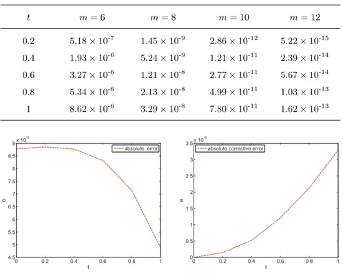
Table 2 shows the absolute errors between the exact solution and approxi-mate solutions of our method for different values of m. From Table 2, we can

Table 2: Absolute errors for different values of m for Example 2. t m = 6 m = 8 m = 10 m = 12 0.2 5.18× 10-7 _{1.45× 10}-9 _{2.86× 10}-12 _{5.22× 10}-15 0.4 1.93× 10-6 5.24× 10-9 1.21× 10-11 2.39× 10-14 0.6 3.27× 10-6 _{1.21× 10}-8 _{2.77× 10}-11 _{5.67× 10}-14 0.8 5.34× 10-6 _{2.13× 10}-8 _{4.99× 10}-11 _{1.03× 10}-13 1 8.62× 10-6 3.29× 10-8 7.80× 10-11 1.62× 10-13 0 0.2 0.4 0.6 0.8 1 4.5 5 5.5 6 6.5 7 7.5 8 8.5 9x 10 -3 t e absolute error 0 0.2 0.4 0.6 0.8 1 0 0.5 1 1.5 2 2.5 3 3.5x 10 -8 t e

absolute corrective error

Figure 1: The absolute errors for m = 4, and the absolute corrective errors for m = 4, me = 8 for Example 2.

say that the numerical solutions come close to the exact solution with the in-creasing value of m. In Figure 1, the absolute errors of our method are given for m = 4. And the errors are not perfect enough. By doing correction for the

345

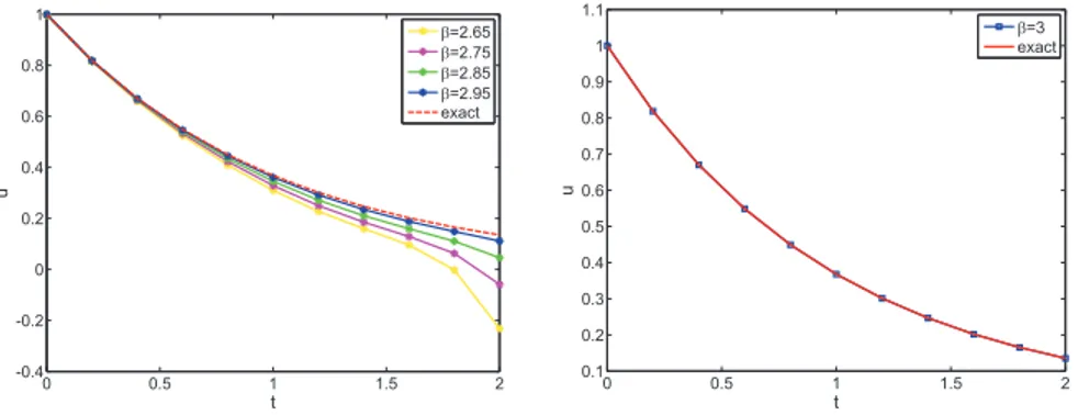
numerical solutions for m = 4, me = 8, the absolute corrective errors achieve about 10-8_{. Figure 2 displays the computational results for m = 7 on [0, 2]}

when β takes different values. By comparing these computational results with exact solution, it is evident from Figure 2 that as β approaches 3, the numerical solutions converge to those of integer order differential equations.

350

Example 3. Consider the fractional multi-pantograph differential equation [33] Dβu (t) =−5 6u (t) + 4u ( 1 2t ) + 9u ( 1 3t ) + t2− 1, 0 < β ≤ 1, u (0) = 1.

0 0.5 1 1.5 2 -0.4 -0.2 0 0.2 0.4 0.6 0.8 1 t u E=2.65 E=2.75 E=2.85 E=2.95 exact 0 0.5 1 1.5 2 0.1 0.2 0.3 0.4 0.5 0.6 0.7 0.8 0.9 1 1.1 t u E=3 exact

Figure 2: The comparison of u (t) for m = 7, with β = 2.65, 2.75, 2.85, 2.95, 1, and the exact solution for Example 2.

In the case, when β = 1, the exact solution is u (t) = 1 +67₆t +1675₇₂ t2₊12157 1296t

3_.

Table 3: The absolute errors for various intervals for Example 3.

t [0, 5] [0, 10]

GFBWFs method Present method GFBWFs method Present method 0 1.60× 10-10 5.34× 10-12 1.31× 10-9 7.28× 10-12 1 5.49× 10-9 _{4.31× 10}-10 _{5.31× 10}-8 _{4.13× 10}-10 2 2.33× 10-8 1.93× 10-9 2.26× 10-7 1.48× 10-9 3 3.31× 10-6 5.36× 10-9 5.85× 10-7 3.05× 10-9 4 1.20× 10-5 _{1.16× 10}-8 _{1.19× 10}-6 _{4.98× 10}-9 5 5.18× 10-7 2.14× 10-8 2.13× 10-6 7.12× 10-9

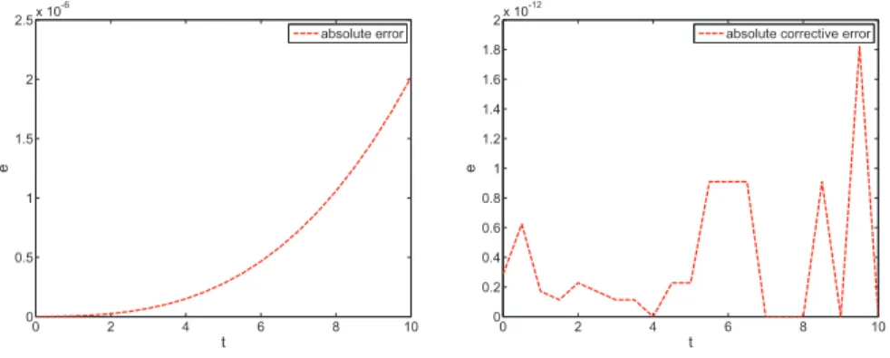
In Table 3, we compare the absolute errors of our method for m = 3 with those of the GFBWFs method of [33] for k = 2, M = 4 on various intervals. Figure 3 gives the numerical results for different choices of β with m = 3 on

355

the interval [0, 10]. The Figure 4 shows the absolute errors between the exact solution and approximate solutions for m = 3, β = 1 on [0, 10] , and the absolute corrective errors between the exact solution and corrective solutions for

m = 3, me = 3 . These results explained that as β approaches 1, the numerical

solutions converge to the exact solution. And it is evident from Figure 4 that

360

0 2 4 6 8 10 0 0.5 1 1.5 2 2.5 3x 10 4 t u E=0.75 E=0.85 E=0.95 exact

Figure 3: The comparison of u (t) for m = 3, with β = 0.75, 0.85, 0.95, and the exact solution for Example 3.

to exact solution than numerical solutions.

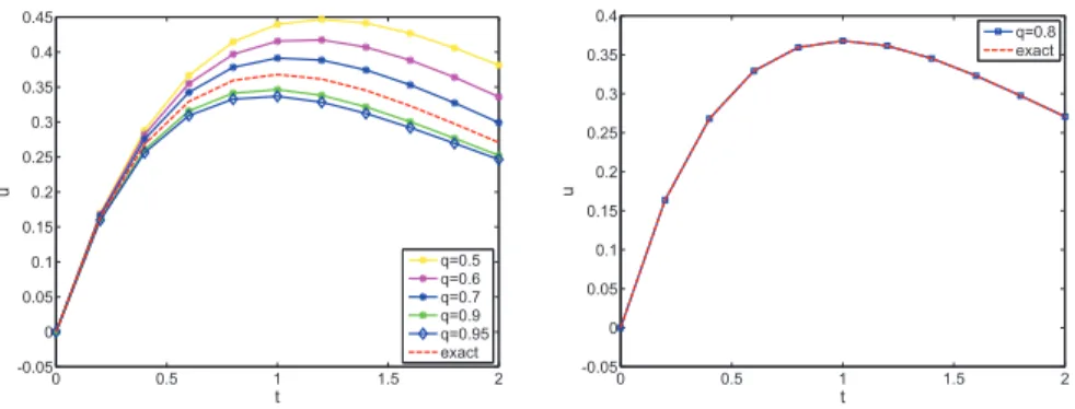
Example 4. Consider the fractional neutral pantograph differential equation Dβu (t) =−u (t) + 0.1u (qt) + 0.5Dβu (qt) + (0.32t− 0.5) e−0.8t+ e−t, 0 < β ≤ 1, u (0) = 0.

In the case, when β = 1, q = 0.8, the exact solution is u (t) = te−t.

0 2 4 6 8 10 0 0.5 1 1.5 2 2.5x 10 -6 t e absolute error 0 2 4 6 8 10 0 0.2 0.4 0.6 0.8 1 1.2 1.4 1.6 1.8 2x 10 -12 t e

absolute corrective error

Figure 4: The absolute errors for m = 3, and the absolute corrective errors for m = 3, me = 3 for Example 3.

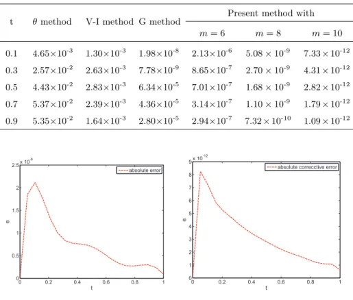
In Table 4, the compassion, the absolute errors of the proposed method

365

variational iteration method (V-I method) [37] form = 6, and the GFBWFsb

method (G method) [33] for k = 2, M = 6 on the interval [0, 1], is given.In Figure 5, we do correction for the numerical solutions with m = 6, and obtain the absolute corrective errors for m = 6, me = 10. Also, the Figure 6 displays the

370

numerical results for m = 10, β = 1 on [0, 2], when q takes different values. And by comparing these results and exact solution, we can see that, as q approaches 0.8, the numerical solutions converge to the exact solution.

Table 4: The comparison of the absolute errors with other methods for Example 4.

t θ method V-I method G method Present method with

m = 6 m = 8 m = 10 0.1 4.65×10-3 1.30×10-3 1.98×10-8 2.13×10-6 5.08× 10-9 7.33×10-12 0.3 2.57×10-2 _2.63×10-3 _7.78×10-9 _8.65×10-7 _{2.70× 10}-9 _4.31×10-12 0.5 4.43×10-2 2.83×10-3 6.34×10-5 7.01×10-7 1.68× 10-9 2.82×10-12 0.7 5.37×10-2 _2.39×10-3 _4.36×10-5 _3.14×10-7 _{1.10× 10}-9 _1.79×10-12 0.9 5.35×10-2 _1.64×10-3 _2.80×10-5 _2.94×10-7 _7.32×10-10 _1.09×10-12 0 0.2 0.4 0.6 0.8 1 0 0.5 1 1.5 2 2.5x 10 -6 t e absolute error 0 0.2 0.4 0.6 0.8 1 0 1 2 3 4 5 6 7 8 9x 10 -12 t e

absolute correcctive error

Figure 5: The absolute errors for m = 6, and the absolute corrective errors for m = 6,

0 0.5 1 1.5 2 -0.05 0 0.05 0.1 0.15 0.2 0.25 0.3 0.35 0.4 0.45 t u q=0.5 q=0.6 q=0.7 q=0.9 q=0.95 exact 0 0.5 1 1.5 2 -0.05 0 0.05 0.1 0.15 0.2 0.25 0.3 0.35 0.4 t u q=0.8 exact

Figure 6: The comparison of u (t) for m = 10, β = 1 with q = 0.5, 0.6, 0.7, 0.8, 0.9, 0.95, and the exact solution for Example 4.

8. Conclusion

In this article, applying the properties of the shifted Chebyshev

polyno-375

mials, we have derived the generalized pantograph operational matrix. Also, according to the SCPs fractional differential operational matrix, the generalized pantograph operational matrix of fractional-order differentiation is introduced. These matrices combined with collocation method are used to simplify and effec-tively calculate the numerical solutions of the generalized fractional pantograph

380

delay equations. By constructing the generalized fractional pantograph delay equations of error function, we obtain the approximate error function to correct numerical solutions . Numerical examples show our method is effective. From examples, it is seen that with the increasing value of m, the absolute error is smaller and the convergence effect between the numerical solutions and the

ex-385

act solution is better. The corrective solutions have better convergence to exact solutions than the numerical solutions. In addition, we find that the present method is an excellent mathematical method, when the function defined on the interval [0, L] and various order β > 0.

Acknowledgements

390

This work is supported by the Natural Science Foundation of Hebei Province (A2017203100) in China and the LE STUDIUM RESEARCH

PROFESSOR-SHIP award of Centre-Val de Loire region in France.

References

[1] F. Mainardi, Fractional calculus and waves in linear viscoelasticity, Imperial

395

College Press, London. 2010.

[2] R.L. Bagley, P.J. Torvik, A theoretical basis for the application of fractional calculus to viscoelasticity, J. Rheology. 27 (3) (1983) 201-210.

[3] R.T. Baillie, Long memory processes and fractional integration in econo-metrics, J. Econometrics. 73 (1996) 5-59.

400

[4] D.Y. Liu, G. Zheng, D. Boutat, H.R. Liu, Non-asymptotic fractional order differentiator for a class of fractional order linear systems, Automatica. 78 (2017) 61-71.

[5] X. Wei, D.Y. Liu , D. Boutat, Non-asymptotic state estimation for a class of fractional order linear systems, IEEE Trans. Autom. Control. 62 (3)

405

(2017) 1150-1164.

[6] F. Mainardi, Fractional relaxation-oscillation and fractional diffusion-wave phenomena, Chaos Solitons Fract. 7 (9) (1996) 1461-1477.

[7] D.Y. Liu, O. Gibaru, W. Perruquetti, T.M. Laleg-Kirati, Fractional order differentiation by integration and error analysis in noisy environment, IEEE

410

Trans. Autom. Control. 60 (11) (2015) 2945-2960.

[8] M.M. Khader, N.H. Sweilam, A.M.S. Mahdy, Numerical study for the fractional differential equations generated by optimization problem using Chebyshev collocation method and FDM, Int. J. Pure Appl. Math. 7 (2013) 2011-2018.

415

[9] S. Kaze, Exact solution of some linear fractional differential equations by Laplace transform, Int. J. Nonlinear Sci. 16 (2013) 3-11.

[10] V.S. Ertrk, S. Momani, Solving systems of fractional differential equations using differential transform method, J. Comput. Appl. Math. 215 (1) (2007) 142-151.

420

[11] X.J. Yang, J.A.T. Machado, H.M. Srivastava, A new numerical technique for solving the local fractional diffusion equation: two-dimensional extended differential transform approach, Appl. Math. Comput. 274 (2016) 143-151. [12] S. Momani, K. Al-Khaled, Numerical solutions for systems of fractional differential equations by the decomposition method, Appl. Math. Comput.

425

162 (3) (2005) 1351-1365.

[13] A. Saadatmandi, M. Dehghan, A new operational matrix for solving fractional-order differential equations, Comput. Math. Appl. 59 (3) (2010) 1326-1336.

[14] H. Saeedi, M. Mohseni Moghadam, Numerical solution of nonlinear

Volter-430

ra integro-differential equations of arbitrary order by CAS wavelets, Non-linear Sci. Numer. Simul. 16 (3) (2011) 1216-1226.

[15] W.G. Ajello, H.I. Freedman, J. Wu, A model of stage structured population growth with density depended time delay, SIAM J. Appl. Math. 52 (1992) 855-869.

435

[16] M.D. Buhmann, A. Iserles, Stability of the discretized pantograph differ-ential equation, Math. Comp. 60 (1993) 575-589.

[17] E.H. Doha, A.H. Bhrawy, S.S. Ezz-Eldien, A Chebyshev spectral method based on operational matrix for initial and boundary value problems of fractional order, Comput. Math. Appl. 62 (2011) 2364-2373.

440

[18] M.A. Ramadan, A.E.A. El-Sherbeiny, M.N. Sherif, Numerical solution of system of first-order delay differential equations using polynomial spline functions, Int. J. Comput. Math. 83 (12) (2006) 925-937.

[19] S. Sedaghat, Y. Ordokhani, M. Dehghan, Numerical solution of the de-lay differential equations of pantograph type via Chebyshev polynomials,

445

Commun. Nonlinear Sci. Numer. Simul. 17 (12) (2012) 4815-4830.

[20] E. Tohidi, A.H. Bhrawy, K.A. Erfani, A collocation method based on Bernoulli operational matrix for numerical solution of generalized panto-graph equation, Appl. Math. Model. 37 (6) (2013) 4283-4294.

[21] Z.H. Yu, Variational iteration method for solving the multi-pantograph

450

delay equation, Phys. Lett. A. 372 (43) (2008) 6475-6479.

[22] C.M. Huang, S. Vandewalle, Discretized stability and error growth of the nonautonomous pantograph equation, SIAM J. Numer. Anal. 42 (5) (2005) 2020-2042.

[23] R.I. Magin, Fractional calculus models of compled dynamics in biological

455

tissnes, Comput. Math. Appl. 59 (2010) 1586-1593.

[24] B.P. Moghaddam, Z.S. Mostaghim, A numerical method based on finite difference for solving fractional delay differential equations, J. Taibah Univ. Sci. 7 (3) (2013) 120-127.

[25] M.L. Morgado, N.J. Ford, P.M. Lima, Analysis and numerical methods for

460

fractional differential equations with delay, J. Comput. Appl. Math. 252 (2013) 159-168.

[26] U. Saeed, M.U. Rehman, Hermite wavelet method for fractional delay dif-ferential equations, J. Diff. Equa. 2014 (1) (2014) 1-8.

[27] M.N. Sherif, I. Abouelfarag, T.S. Amer, Numerical solution of fractional

465

delay differential equations using Spline functions, Int. J. Pure Appl. Math. 90 (1) (2014) 73-83.

[28] M.A. Iqbal, U. Saeed, S.T. Mohyud-Din, Modified Laguerre Wavelets method for delay differential equations of fractional-order, Egypt. J. Basic Appl. Sci. 2 (1) (2015) 50-54.

[29] U. Saeed, M.U. Rehman, M.A. Iqbal, Modified Chebyshev wavelet methods for fractional delay-type equations, Appl. Math. Comput. 264 (2015) 431-442.

[30] P. Rahimkhani, Y. Ordokhani, E. Babolian, A new operational matrix based on Bernoulli wavelets for solving fractional delay differential

equa-475

tions, Numer. Algor. 74 (1) (2016) 223-245.

[31] K. Balachandran, S. Kiruthika. Existence of solutions of nonlinear fraction-al pantograph equations, Acta Math. Sci. 33 (2013) 712-720.

[32] Y. Yang, Y.Q. Huang, Spectral-collocation methods for fractional panto-graph delay-integrodifferential equations, Adv. Math. Phys. 2013 (2013)

480

1-14.

[33] P. Rahimkhani, Y. Ordokhani, E. Babolian, Numerical solution of fraction-al pantograph differentifraction-al equations by using generfraction-alized fractionfraction-al-order Bernoulli wavelet, J. Comput. Appl. Math. 309 (2016) 493-510.

[34] Z.J. Hei, A method of solving inverse of a matrix, Journal of Harbin

Insti-485

tute of Technology. 36 (10) (2004) 1351-1353.

[35] M. Sezer, S. Yalcinbas, M.Culsu, A Taylor polynomial approach for solv-ing generalized pantograph equations with nonhomogeneous term, Int. J. Comput. Math. 85 (7) (2008) 1055-1063.

[36] W.S. Wang, S.F. Li, On the one-leg θ-methods for solving nonlinear neutral

490

functional differential equations, Appl. Math. Comput. 193 (1) (2007) 285-301.

[37] X. Chen, L. Wang, The variational iteration method for solving a neutral functional-differential equation with proportional delays, Comput. Math. Appl. 59 (8) (2010) 2696-2702.