Active learning for electrodermal activity classification

Active learning for electrodermal activity classification

The MIT Faculty has made this article openly available.

Please share

how this access benefits you. Your story matters.

Citation

Xia, Victoria, Natasha Jaques, Sara Taylor, Szymon Fedor, and

Rosalind Picard. “Active Learning for Electrodermal Activity

Classification.” 2015 IEEE Signal Processing in Medicine and Biology

Symposium (SPMB) (December 2015).

As Published

http://dx.doi.org/10.1109/SPMB.2015.7405467

Publisher

Institute of Electrical and Electronics Engineers (IEEE)

Version

Author's final manuscript

Citable link

http://hdl.handle.net/1721.1/109392

Terms of Use

Creative Commons Attribution-Noncommercial-Share Alike

Active Learning for Electrodermal Activity Classification

Victoria Xia

, Natasha Jaques

, Sara Taylor

, Szymon Fedor

, and Rosalind Picard

Abstract— To filter noise or detect features within physio-logical signals, it is often effective to encode expert knowledge into a model such as a machine learning classifier. However, training such a model can require much effort on the part of the researcher; this often takes the form of manually labeling portions of signal needed to represent the concept being trained. Active learning is a technique for reducing human effort by developing a classifier that can intelligently select the most relevant data samples and ask for labels for only those samples, in an iterative process. In this paper we demonstrate that active learning can reduce the labeling effort required of researchers by as much as 84% for our application, while offering equivalent or even slightly improved machine learning performance.

I. INTRODUCTION

In order to extract meaningful information from physio-logical signals, researchers are often forced to painstakingly review large quantities of signal data in order to determine which portions contain poor quality signal or noise, and which contain useful information. In the case of large-scale studies which gather hundreds of thousands of hours of noisy, ambulatory data (e.g., [22]), this is extremely impractical. For this reason, recent research efforts have focused on training automated algorithms to recognize noise in physiological signals, including electrocardiogram (ECG) (e.g., [16], [17], [27]), electrodermal activity (EDA) (e.g., [28]), and electroencephalography (EEG) (e.g., [30]). While these automated techniques have proven successful, training them still requires a large amount of effort on the part of human researchers. 02:22:24 02:22:54 02:23:24 02:23:54 02:24:24 Time 0.50 0.55 0.60 0.65 0.70 µS

Fig. 1. Raw EDA signal containing normal skin conductance responses

(SCRs) that occur in response to temperature, exertion, stress, or emotion. This research focuses on more efficiently training auto-matic algorithms to extract meaningful information from electrodermal activity (EDA) data. EDA refers to electrical activity on the surface of the skin, which increases in response to exertion, temperature, stress, or strong emotion

1_{Affective Computing Group, Media Lab, Massachusetts Institute of}

Technology, 75 Amherst Street, Cambridge, U.S.{vxia, jaquesn,

sataylor, sfedor, roz}@mit.edu

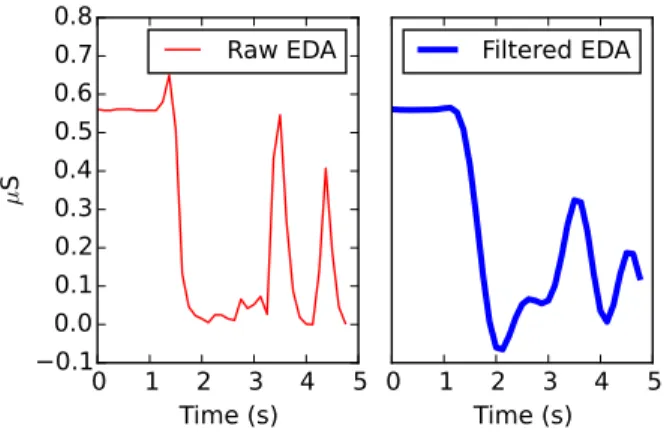
[2]. For this reason, EDA has been frequently used to study emotion and stress (e.g., [12], [13], [23]). Improvements in the devices used to monitor EDA have allowed for 24-hour-a-day, ambulatory monitoring, enabling important research into how the body responds physiologically to stress and emotional stimuli during daily life [22]. However, this type of in-situ monitoring comes at a price; ambulatory EDA is often too voluminous to be inspected by hand, and noisy, containing artifacts generated from fluctuations in contact or pressure between the sensor and the skin. In order to extract meaningful information from this data, it is important to au-tomatically distinguish between skin conductance responses (SCRs) (which may indicate increased stress or emotion), and noise (see Figures 1 and 2).

0 1 2 3 4 5

Time (s)

−0.1

0.0

0.1

0.2

0.3

0.4

0.5

0.6

0.7

0.8

S

Raw EDA

0 1 2 3 4 5

Time (s)

Filtered EDA

Fig. 2. This figure shows a typical artifact, where the left side of the figure is the raw signal, and the right side is the signal after applying a low-pass

Butterworth filter (order= 6, f0= 1 Hz). Simple filtering and smoothing

is insufficient to remove artifacts.

Typical methods for removing noise from EDA signal involve exponential smoothing (e.g., [9]) or low-pass filtering (e.g., [10], [13], [20], [23]); these techniques are unable to deal with large-scale artifacts such as those shown in Figure 2, and may result in these artifacts being mistaken for SCRs. Similarly, commonly employed heuristic techniques for detecting SCRs (e.g., [1], [26], [24]) are also error prone. A more effective approach is to encode the knowledge of human experts into a mathematical model or machine learning algorithm (e.g., [5], [18], [28]). This approach was successfully used to train a machine learning classifier that could identify artifacts in an EDA signal with over 95% accuracy [28]. However, encoding this knowledge required significant effort; two experts had to label over 1500 five-second epochs of EDA data to achieve this recognition rate [28]. Further, this type of encoding can lead to a highly specific model that cannot generalize to other applications.

Active learning is a promising technique for encoding ex-pert knowledge in a machine learning classifier with minimal human effort. Rather than require an expert researcher to label a dataset of thousands of examples, an active learning classifier can intelligently select which samples would be most informative to the classification problem, and only request labels for those. This paper will explore how to employ active learning in two different problems within the domain of EDA signal processing: artifact detection and detection of SCRs. Both problems showed promising results.

II. BACKGROUND

The following sections will introduce concepts and previ-ous work related to the machine learning and active learning algorithms we use in this research.

A. Support Vector Machines

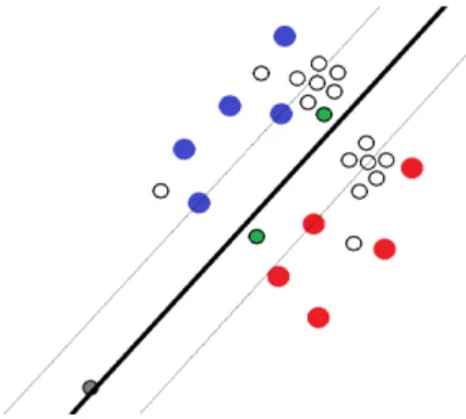
Support Vector Machines (SVMs) are a machine learning classification algorithm that have been found to be highly effective with active learning [14] [25] [29]. SVMs work by finding a decision boundary that separates one class from another (e.g., SCR vs. non-SCR). For a separable dataset, there are many possible decision boundaries that could divide the data into the two classes. SVMs choose the boundary that maximizes the size of the margin, the space between the decision boundary hyperplane and the points closest1 to it (see Figure 3 for an illustration of this concept) [8]. B. Active Learning

The purpose of active learning is to intelligently select data samples that can be used to train an effective machine learning classifier, so not all samples have to be labeled by human experts. In pool-based active learning, the active learner selects batches of data samples, or query sets, for which to request labels, from a provided collection of unla-beled samples.

A reasonable way to obtain the initial batch is to cluster the data, and include the samples closest to the centroid of each cluster in the first query set [11]. This approach allows the classifier to begin developing a representative decision boundary; increasing the number of clusters improves the initial decision boundary, but requires the human expert to provide more labels. Various strategies can then be used to select successive query sets. We will introduce several below based on active learning with SVMs. After each query set, the SVM is re-trained, and the new decision boundary produced is used to help evaluate which data samples should be included in the next query set.

The following are various SVM-based query strategies: 1) Simple Margin: This strategy is one of many uncer-tainty samplingalgorithms. Uncertainty sampling techniques choose to query samples the classifier is unsure how to label, with the expectation that learning how to label these samples will improve the classifier the most [15]. In the case of SVMs, one heuristic for how uncertain the classifier is about

1_{Here “closest” is a measure of distance defined by the feature space and}

kernel function.

Fig. 3. The SVM decision boundary is shown as the thick black line, and

the margin is the distance between the thin lines to either side. Large red and blue points represent those samples that have been labeled (into one of two possible classes), while small points are unlabeled samples. Though the gray point may be an outlier, Simple Margin would choose to query it first. In contrast, Mirroshandel et al.’s method queries the green points first.

each sample is the distance of the sample to the decision boundary. Thus, Simple Margin queries the samples closest to the decision boundary of the SVM [3].

2) Mirroshandel’s Algorithm (2011): As shown in Figure 3, a drawback of Simple Margin is that it may query outliers. To prevent this, Mirroshandel et al. [19] proposed balancing uncertainty with representativeness, by combining distance to the decision boundary (uncertainty) with average distance to the other samples (representativeness). These factors are combined by placing a weight of α on uncertainty and 1 − α on representativeness.

3) Xu’s Algorithm (2003): Na¨ıvely querying the sam-ples closest to the decision boundary (as Simple Margin does) is problematic, both because these samples may not be representative of the other samples (the motivation for Mirroshandel’s algorithm), but also because these samples may be redundant among themselves. To remedy both these issues, Xu et al. [32] proposed running a clustering algorithm on the samples near the decision boundary, and then querying the centers of each cluster. Samples chosen using this method will be close to the boundary, likely representative of the surrounding samples, and different from each other. Xu’s algorithm chooses to cluster on samples within the margin.

4) MaxMin Margin: Another uncertainty sampling tech-nique, MaxMin Margin seeks to more intelligently shrink the space of consistent decision boundaries (i.e., version space) by maximizing the guaranteed change in version space size with each query. To do so, MaxMin Margin follows the algorithm below [29]:

1) For each unlabeled sample, i:

a) Treat i as a positive example. Compute m+_i , the size of the resulting margin.

b) Treat i as a negative example. Compute m−_i , the size of the resulting margin.

c) Find the minimum of m+_i and m−_i . Call it mi.

2) Query the samples that have the greatest mi values.

3) Repeat 1) and 2) until some stopping criterion is reached.

C. Automatic Stopping Criterion

Because the goal of active learning is to allow experts to label only a fraction of the data required for supervised learning, an important question is how to decide when enough samples have been queried. One option would be to allow human experts to periodically evaluate the performance of the classifier and stop when satisfied, but this is unreliable and time-consuming. Ideally, the active learner itself would be able to suggest a stopping point. Schohn and Cohn [25] proposed a simple stopping criterion that has been empirically proven to be highly effective: continue querying until all samples within the margin of the SVM have been labeled.

III. DATACOLLECTION A. Dataset I

Building on previous work [28], we began by applying active learning to the problem of artifact detection in EDA. We use the same dataset that was analyzed in the the original work [28], which was obtained from a study in which par-ticipants wore Affectiva Q EDA sensors while experiencing physical, cognitive and emotional stressors [6]. The collected data were split into non-overlapping five-second epochs; 1560 epochs were selected for expert labeling. Two experts labeled each epoch as either containing an artifact or not based on an agreed-upon set of criteria, using the procedure described in Section IV-A.

B. Dataset II

In order to provide a more robust test of the effectiveness of active learning, we obtained novel data collected in a different setting, for a different application, using a different sensor—the Empatica E4. The study collected data from participants while they were sleeping at home. A total of 3001 non-overlapping epochs were labeled by two experts using the procedure described in Section IV-A, but this time epochs were labeled for skin conductance responses (SCRs) rather than for artifacts. The experts agreed beforehand to label SCRs based on Boucsein’s characterization of a typical SCR [2]. Automatically detecting SCRs during sleep could potentially be very useful, especially in studying EDA “sleep storms”, bursts of activity in which many SCRs occur during slow-wave sleep [21].

IV. METHODS A. Expert Labeling

Our experts labeled each epoch as belonging to one of two classes (artifact or non-artifact for Dataset I, SCR or non-SCR for Dataset II) using an online tool we built, EDA Explorer (eda-explorer.media.mit.edu). The site automatically splits raw EDA data into five-second epochs, generates and displays plots for epochs one at a time, and records input labels associated with each plot. For each epoch, the experts were shown a plot of both the raw and low-pass-filtered five-second EDA signal, a context plot showing the surrounding five seconds of signal on either side

(if applicable), and also plots of the relevant accelerometer and temperature signals (collected by the sensor). Using these plots, each expert chose to assign one of two possible labels to the epoch, or skip it (if they did not wish to assign a label).

Note that although the experts were shown accelerometer and temperature plots to aid in their decision-making, this information was not provided to any of our classifiers, as in the original work [28]. By withholding this information from our classifiers, we allow them to generalize to EDA signal collected by any EDA sensor, regardless of whether accelerometer and temperature data were also collected. B. Partitioning Data

For each dataset, epochs which were skipped and those for which the two experts did not agree on a label were removed, following the original work [28]. This choice was made because it is impossible to determine a ground truth classification for epochs on which the experts disagree. Further, we seek to establish the effectiveness of active learning in comparison to previous work on automatic signal classification, and using the same dataset as previous work [28] allows us to do so. For Dataset II, the experts identified four times as many epochs that did not contain an SCR as epochs that did, so we randomly subsampled non-SCR epochs to create a balanced dataset.

In total, Dataset I contained 1050 epochs, and Dataset II contained 1162. The epochs for each dataset were randomly split into training, validation, and test sets in a 60/20/20% ratio. Feature selection was performed using the training data, parameter selection was performed using the validation data, and the testing data was held-out until the algorithms were finalized, and used to provide an estimate of the classifier’s generalization performance.

C. Feature Extraction

From each dataset, we extracted the same features as in the original work [28]. These features included shape features (e.g., amplitude, first and second derivatives) of both the raw signal and the signal after a 1Hz low-pass filter had been applied. We computed additional features by applying a Discrete Haar Wavelet Transform to the signal. Wavelet transforms are a time-frequency transformation; the Haar wavelet transform computes the degree of relatedness between subsequent samples in the original signal, and there-fore can detect edges and sharp changes [31]. We obtained wavelet coefficients at 4Hz, 2Hz, and 1Hz, and computed statistics related to those coefficients for each five-second epoch. At this stage we were unconcerned with redundancy of features, as we later performed feature selection (see Section IV-D). Finally, we standardized each feature to have mean 0 and variance 1 over epochs in the training set. D. Feature Selection

The features provided to the classification algorithm were selected using wrapper feature selection (WFS) applied to

Dataset I, as in the original work [28]. WFS tests clas-sifier performance using different subsets of features, and aims to select the subset of features which yields the best performance [7]. Because this is computationally expensive, we used a greedy search strategy to search through the space of possible subsets. Because feature selection requires knowledge of the true classification label, we did not re-select new features for Dataset II. We reasoned this would be a more robust test of active learning, in which the true classification label of the data samples in the training set is not known in advance, and allow us to assess how our active learning pipeline will generalize to novel EDA data. E. Active Learning

The previous work on detecting artifacts in an EDA signal explored many different machine learning algorithms [28], and found SVMs to be the most effective. For this reason, and because SVMs make for excellent active learners, we chose to focus on the SVM classifier for this work.

Our active learning methodology is as follows. The initial query set provided to the active learner was determined by running an approximate k-means algorithm to cluster the unlabeled samples into num-clusters clusters, and choosing the sample closest to the centroid of each cluster to be part of the query set2. Subsequent query sets of size batch-size samples were selected using one of four different query strategies. After assessing the effectiveness of a range of values, we selected num-clusters = 30 and batch-size = 5.

The four query strategies we tested were discussed above (in II-B): Simple Margin, Mirroshandel’s representativeness algorithm, Xu’s clustering algorithm, and MaxMin Margin. For our implementation of Mirroshandel’s algorithm, we tested α values ranging from 0.40 to 0.75, based on values reported in previous work [19]. For Xu’s algorithm, we experimented with clustering on varying amounts of sam-ples closest to the boundary (e.g., closest 5% of unlabeled samples to the boundary, closest 30 unlabeled samples, etc.). In order to assess whether our active learning methods provide a benefit over a simple passive learner, we also implemented a query strategy which simply chooses the query set randomly. Note that this random sampler still benefits from the initial query set provided by the clustering algorithm. Any improvements upon the random sampler must therefore be due to the benefit of active learning, rather than clustering.

We also assessed the effectiveness of employing the stop-ping criterion presented in Section II-C to the Simple Margin query strategy. We did not test it with the other techniques; the criterion does not apply well to them, since they are not are not guaranteed to query samples within the margin first.

V. RESULTS

Because the approximate clustering algorithm used to se-lect the initial query set contains randomness, query sets (and

2_{In the event that the same sample was chosen multiple times, the next}

closest sample not yet in the query set was added to the query set instead.

consequently, classifier performance) vary across different runs of the algorithm. Thus, all of our reported results are averaged over 100 runs. We report our results in terms of accuracy; that is, the proportion of correctly classified examples in the validation or test set.

A. Dataset I - Artifacts

We began by searching the parameter space of each active learning algorithm to find the values that gave the best performance on the validation set. For Xu’s clustering algorithm, we found clustering on the 30 samples closest to the margin to be most effective. For the representativeness algorithm, α = 0.65 was found to give the best performance, which agrees with what was found previously [19].

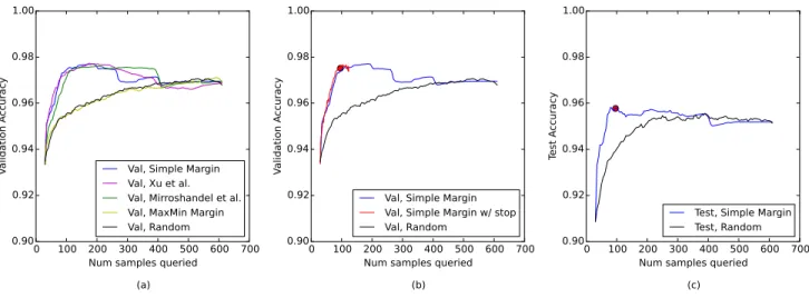
Figure 4(a) shows the performance of each strategy in classifying artifacts in Dataset I. We see that three of the techniques outperform the Random baseline, indicating that active learning on this problem is highly effective. Using Simple Margin, for example, a higher validation accuracy is obtained after only 100 samples have been labeled than is ever obtained by passive learning. After this initially high performance, the accuracy of Simple Margin drops steadily to meet the level of the classifier trained on the entire dataset. Others have observed this phenomenon as well (e.g., [4], [25]). We suspect the initially superior performance of the active learning methods may be due to their ability to successfully query relevant samples. As the rest of the data, including irrelevant examples, are added to the classifier, the classifiers may begin to overfit to the training data [4].

In comparing the performance of Simple Margin with that of the Xu’s and Mirroshandel’s algorithm, we see that they are roughly equivalent for the first 300 samples. After this point, Mirroshandel’s and Xu’s algorithm appear to outper-form Simple Margin. Because the goal of active learning is to have the human researcher label as few examples as possible, this later performance difference is of little interest. However, we can see from Figure 4(a) that MaxMin Margin does not offer a performance improvement over Random Sampling. We suspect this is because our dataset may not be separable, due to a combination of noise and having only selected nine features, thus violating the separability assumption of MaxMin Margin [29].

Figure 4(b) and Table I show the results obtained using Schohn and Cohn’s automatic stopping criterion. On average, the algorithm chose to stop after only 96.7 samples had been queried, and ended with an average validation accuracy greater than that achieved using the entire training set and reported in the original work [28]. Because this stopping criterion is so effective, we chose to apply Simple Margin with this criterion to the testing data to obtain a final estimate of the ability of our technique to generalize to novel data. Figure 4(c) shows the accuracy obtained on the held-out test dataset. As with the validation set, Simple Margin with Schohn and Cohn’s automatic stopping criterion ended, on average, with a test accuracy higher than that achieved by training on the entire training set. This suggests that with active learning, the same (or even slightly better)

0 100 200 300 400 500 600 700 Num samples queried

(a) 0.90 0.92 0.94 0.96 0.98 1.00 Va lid ati on Ac cu rac y

Val, Simple Margin Val, Xu et al. Val, Mirroshandel et al. Val, MaxMin Margin Val, Random

0 100 200 300 400 500 600 700 Num samples queried

(b) 0.90 0.92 0.94 0.96 0.98 1.00 Va lid ati on Ac cu rac y

Val, Simple Margin Val, Simple Margin w/ stop Val, Random

0 100 200 300 400 500 600 700 Num samples queried

(c) 0.90 0.92 0.94 0.96 0.98 1.00 Te st Ac cu rac y

Test, Simple Margin Test, Random

Fig. 4. (a) Validation accuracies of various query strategies tested on the artifacts dataset; (b) Validation performance of Schohn and Cohn’s automatic

stopping criterion on the artifacts dataset. The large red dot marks the average number of samples queried before the algorithm chose to stop, and the average ending validation accuracy; (c) Generalization performance (test accuracy) of Simple Margin with Schohn and Cohn’s automatic stopping criterion, on the artifacts dataset. The large red dot marks the average number of samples queried and the average ending test accuracy.

TABLE I

RESULTS OFSIMPLEMARGIN(WITH THESTOPPINGCRITERION)ON

THEARTIFACTSDATASET

Samples Queried Val. Acc. Test Acc.

Active Learner 96.7 0.975 0.958

Passive Learner 612 0.970 0.952

classification performance can be achieved with one-sixth the number of labeled training epochs, allowing for a large reduction in the amount of labor required of human experts. B. Dataset II - Peaks

To demonstrate that active learning is also effective for novel problems and novel sensor technologies, we apply the same methodology to Dataset II in order to detect SCRs within an EDA signal. In this case, we found clustering on the 5% of peaks closest to the decision boundary to be most effective with Xu’s algorithm, and once again found α = 0.65 to work best with Mirroshandel’s algorithm.

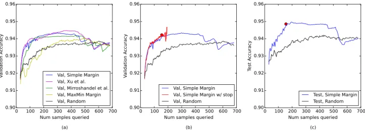
As shown in Figure 5(a), we observed similar relative performance of the various query strategies for this second dataset as for the first. Note that the performance advantage offered by additional training data is smaller. We suspect this is because the problem is easier; SCRs tend to have a consistent shape whereas artifacts and noise can vary. Schohn and Cohn’s automatic stopping criterion performed well once again (see Figures 5(b) and Table II). On average, the algorithm stopped after 155.4 samples (23% of the entire training set), and still achieved slightly better performance than training on the entire dataset. In Figure 5(c), we plot the performance of the active learner on the held-out test dataset. We can see once again that the generalization performance of active learning is higher than that of passive learning, yet requires only 23% of the effort on the part of human researchers.

TABLE II

RESULTS OFSIMPLEMARGIN(WITH THESTOPPINGCRITERION)ON

THEPEAKSDATASET

Samples Queried Val. Acc. Test Acc.

Active Learner 155.4 0.942 0.949

Passive Learner 682 0.939 0.941

VI. CONCLUSION ANDFUTUREWORK

We have shown that active learning is a promising tech-nique for reducing the labeling effort required to train a machine learning algorithm in signal classification. In our case, the active learner can achieve equivalent or even slightly superior performance using as little as 16% of the data. We found Simple Margin to be an effective and reliable strategy, which if deployed with Schohn and Cohn’s stopping criteria can automatically determine when to stop querying for more labels. The results from Dataset II are of particular interest because they correspond to the performance we can expect when employing our active learning techniques on a novel EDA dataset.

Though our exploration focused on EDA signals, our techniques could likely be extended to other types of signals, such as ECG or photoplethysmogram (PPG). We are also planning to incorporate our active learning algorithm into the online tool we have built for processing EDA signals, eda-explorer.media.mit.edu. Researchers will be able to use our site to label data to train a classifier, while the active learner intelligently selects which epochs need to be labeled. Future work may also include extending the active learning techniques for EDA signal classification discussed here to multiclass classification. For example, we may be interested in classifying epochs into one of three categories: artifact, SCR, or neither.

0 100 200 300 400 500 600 700 Num samples queried

(a) 0.90 0.91 0.92 0.93 0.94 0.95 0.96 Va lid ati on Ac cu rac y

Val, Simple Margin Val, Xu et al. Val, Mirroshandel et al. Val, MaxMin Margin Val, Random

0 100 200 300 400 500 600 700 Num samples queried

(b) 0.90 0.91 0.92 0.93 0.94 0.95 0.96 Va lid ati on Ac cu rac y

Val, Simple Margin Val, Simple Margin w/ stop Val, Random

0 100 200 300 400 500 600 700 Num samples queried

(c) 0.90 0.91 0.92 0.93 0.94 0.95 0.96 Te st Ac cu rac y

Test, Simple Margin Test, Random

Fig. 5. (a) Validation accuracies of various query strategies tested on the peaks dataset; (b) Validation performance of Schohn and Cohn’s automatic

stopping criterion on the peaks dataset. The large red dot marks the average number of samples queried before the algorithm chose to stop, and the average ending validation accuracy; (c) Generalization performance (test accuracy) of Simple Margin with Schohn and Cohn’s automatic stopping criterion, on the peaks dataset. The large red dot marks the average number of samples queried and the average ending test accuracy.

ACKNOWLEDGMENT

This work was supported by the MIT Media Lab Con-sortium, the Robert Wood Johnson Foundation, Canada’s NSERC program, and the People Programme of the Euro-pean Union’s Seventh Framework Programme.

REFERENCES

[1] S. Blain et al. Assessing the potential of electrodermal activity as an alternative access pathway. Medical engineering & physics, 30(4):498– 505, 2008.

[2] W. Boucsein. Electrodermal activity. Springer Science+Business

Media, LLC, 2012.

[3] C. Campbell et al. Query learning with large margin classifiers. In ICML, pages 111–118, 2000.

[4] J. Chen et al. An empirical study of the behavior of active learning for word sense disambiguation. In Proc. of HLT/NAACL, pages 120–127. ACL, 2006.

[5] W. Chen et al. Wavelet-based motion artifact removal for electrodermal activity. In EMBC. IEEE, 2015.

[6] S. Fedor and R. Picard. Ambulatory eda: Comparison of bilateral fore-arm and calf locations. In Society for Psychophysiological Research (SPR), 2014.

[7] I. Guyon and A. Elisseeff. An introduction to variable and feature selection. The Journal of Machine Learning Research, 3:1157–1182, 2003.

[8] M. A. Hearst et al. Support vector machines. Intelligent Systems and their Applications, IEEE, 13(4):18–28, 1998.

[9] J. Hernandez et al. Call center stress recognition with person-specific models. In ACII, pages 125–134. Springer, 2011.

[10] J. Hernandez et al. Using electrodermal activity to recognize ease of engagement in children during social interactions. In Pervasive and Ubiquitous Computing, pages 307–317. ACM, 2014.

[11] J. Kang et al. Using cluster-based sampling to select initial training set for active learning in text classification. In Advances in knowledge discovery and data mining, pages 384–388. Springer, 2004. [12] C. Kappeler-Setz et al. Towards long term monitoring of electrodermal

activity in daily life. Pervasive and Ubiquitous Computing, 17(2):261– 271, 2013.

[13] R. Kocielnik et al. Smart technologies for long-term stress monitoring at work. In Comput.Based Medical Syst., pages 53–58. IEEE, 2013. [14] J. Kremer et al. Active learning with support vector machines. Wiley

Interdisciplinary Reviews: Data Mining and Knowledge Discovery, 4(4):313–326, 2014.

[15] D. D. Lewis and W. A. Gale. A sequential algorithm for training text classifiers. In SIGIR Forum, pages 3–12. Springer-Verlag New York, Inc., 1994.

[16] Q. Li et al. Signal quality indices and data fusion for determining acceptability of electrocardiograms collected in noisy ambulatory environments. Computing in Cardiology, 38, 2011.

[17] Q. Li, C. Rajagopalan, and G. D. Clifford. A machine learning

approach to multi-level ecg signal quality classification. Computer methods and programs in biomedicine, 117(3):435–447, 2014. [18] C. L. Lim et al. Decomposing skin conductance into tonic and phasic

components. Int. J. of Psychophysiology, 25(2):97–109, 1997. [19] S. A. Mirroshandel et al. Active learning strategies for support vector

machines, application to temporal relation classification. In IJCNLP, pages 56–64, 2011.

[20] M.-Z. Poh. Continuous assessment of epileptic seizures with wrist-worn biosensors. PhD thesis, MIT, 2011.

[21] A. Sano et al. Quantitative analysis of wrist electrodermal activity during sleep. Int. J. of Psychophysiology, 94(3):382–389, 2014. [22] A. Sano et al. Discriminating high vs low academic performance,

self-reported sleep quality, stress level, and mental health using personality traits, wearable sensors and mobile phones. In Body Sensor Networks, 2015.

[23] A. Sano and R. Picard. Stress recognition using wearable sensors and mobile phones. In ACII, pages 671–676. IEEE, 2013.

[24] A. Sano and R. W. Picard. Recognition of sleep dependent memory consolidation with multi-modal sensor data. In Body Sensor Networks. IEEE, 2013.

[25] G. Schohn and D. Cohn. Less is more: Active learning with support vector machines. In ICML, pages 839–846. Citeseer, 2000. [26] H. Storm et al. The development of a software program for analyzing

spontaneous and externally elicited skin conductance changes in infants and adults. Clin. Neurophysiology, 111(10):1889–1898, 2000. [27] S. Subbiah et al. Feature extraction and classification for ecg signal processing based on artificial neural network and machine learning approach. In Proc. of ICIDRET, 2015.

[28] S. Taylor, N. Jaques, et al. Automatic identification of artifacts in electrodermal activity data. EMBC. IEEE, 2015.

[29] S. Tong and D. Koller. Support vector machine active learning with applications to text classification. The Journal of Machine Learning Research, 2:45–66, 2002.

[30] I. Winkler et al. Automatic classification of artifactual ica-components for artifact removal in eeg signals. Behavioral and Brain Functions, 7(1):30, 2011.

[31] Y. Xu et al. Wavelet transform domain filters: a spatially selective noise filtration technique. Image Processing, 3(6):747–758, 1994.

[32] Z. Xu et al. Representative sampling for text classification using