Air flow effects in the piston ring pack and their implications on oil transport

Air Flow Effects in the Piston Ring Pack and their

Implications on Oil

Transport

ARCHIVES

by

Yuan Wang

Dipl.-Ing., Universitit Stuttgart (2012)

Submitted to the Department of Aeronautics and Astronautics in partial fulfillment of the requirements for the degree of

Master of Science in Aeronautics and Astronautics at the

MASSACHUSETTS INSTITUTE OF TECHNOLOGY September 2012

@

Author... ... ... . .

Pepartment of Aeronautics and A onautics Aug st 15, 2012

C ertified by ... _...

Tian Tian Principal Research Engineer, Department of Mechanical Engineering Thesis Supervisor

A ccepted by ... _....

Eytan H. Modiano Professor fAeronautics and Astronautics Chair, Graduate Program Committee

Air Flow Effects in the Piston Ring Pack and their

Implications on Oil Transport

by

Yuan Wang

Submitted to the Department of Aeronautics and Astronautics on August 15, 2012, in partial fulfillment of the

requirements for the degree of

Master of Science in Aeronautics and Astronautics

Abstract

3 different flow regimes of piston blowby air and their influences on oil transport are

studied. It is found that air mainly interacts with oil close to the ring gaps and directly below the ring-liner contacts. Geometric features at the gaps to smoothen airflow and prevent flow detachments can increase blowby mass flow rate and thus drainage oil mass flow rate by up to 60%. Only oil within 1 to 2 gap widths distance from the gaps are transported through the gap by air drag and the engine pressure drop. Downstream of the ring gap, transported oil will either be caught in vortices directly below the ring gaps or pumped into the downstream ring groove due to the creation of a blowby stagnation point. Far away from the gaps, oil is mainly transported in axial direction through the grooves and the piston-liner interface. Low capillary numbers in the order of 10-- indicate close to no oil transport into circumferential direction from blowby shear. The oil transport radially into the grooves is mainly determined

by hydrostatics and capillary effects in the groove flanks wheras air in the second land

only has an influence on oil transport by preventing bridging after TDC by creating a stagnation point directly below the rings on the liner.

Thesis Supervisor: Tian Tian

Acknowledgments

My main acknoledgements go to my brilliant advisor Dr. Tian Tian for his endless

support and excellent guidance throughout my research. All my motivation and

passion stem from his constant clarity, enthusiasm and experience without which I would have never been able to succeed at MIT.

Furthermore I would like to express all my gratitudes to our sponsors Argonne National Lab, Daimler, DOE, Mahle, Renault, PSA, Toyota, Volkswagen and Volvo, who made this project possible. Specifically I would like to thank Remi for his great humor and training he provided; Bengt, Erich, Hand-Jiirgen, Matthias, Paulo and

Dr. Fiedler for all the fun discussions and motivation; Steve and Eric for taking care of all necessities and providing feedback and Tom for his constructive suggestions.

Thanks a lot to the funnniest and smartest labmates at MIT Camille, Haijie, Kai, Matthieu and Yang. I love the team natured spirit in our office, the sporadic sweet secrets hidden in our fridge and all the great discussions we had. Nowhere else will it

be so fun coming to work every morning. Moreover I would like to thank Janet and Thane for their kindness and assistance during my studies.

Finally I would like to thank my wonderful parents and girlfriend for all their

support and love. They have continuously brought joy and laughter to me during my

Contents

1 Introduction 15

1.1 B ackground . . . . 15

1.1.1 Ring Pack Geometry . . . . 15

1.1.2 Blowby Flow Path in the Piston Ring Pack . . . . 17

1.2 Motivation and Objectives . . . . 19

1.3 Related Research . . . . 19

2 Air flow through ring gaps 21 2.1 Definition of Test Cases . . . . 21

2.1.1 Choking at the first Ring Gap . . . . 21

2.1.2 Relevant Geometry . . . . 23

2.1.3 Computational Domain . . . . 25

2.1.4 Relevant Parameters . . . . 26

2.1.5 Boundary Conditions . . . . 27

2.1.6 Gas Properties and Flow Regime . . . . 29

2.1.7 Governing equations and solution method . . . . 30

2.2 Total Temperature Fields . . . . 32

2.3 Blowby flow at the ring gap . . . . 33

2.4 Variations of C . . . . 35

2.5 Variations of T . . . . 37

2.6 Comparison to Previous Results . . . . 42

3 2nd 3.1 3.2 3.3 3.4 3.5

4 Multiphase interaction in the 3rd land

4.1 M ultiphase solver . . . .

4.1.1 Governing equations and solution method . . . . 4.1.2 Interface approximation . . . . 4.2 Definition of Test Cases . . . . 4.2.1 Computational domain and boundary conditions . 4.2.2 Mesh resolution . . . . 4.3 Pressure effects at the second ring groove inlet . . . .

4.3.1 Hooked second ring with rectangular chamfer . .

4.3.2 Rectangular second ring . . . .

4.4 Conclusions for pressure effects . . . . 4.5 B ridging . . . .

4.5.1 Oil drop flowing up the piston . . . . 4.5.2 Spreading at the second ring . . . .

4.5.3 Geometric variations . . . . 4.5.4 Bridging height . . . . 4.6 Conclusions for bridging . . . .

land air flow

Definition of Test Cases . . . .

3.1.1 Steady choked condition . . . .

3.1.2 Computational domain . . . .

3.1.3 Boundary conditions . . . .

3.1.4 Governing equations and solution method Oil accumulation at the inlet gap . . . .

Air flow far away from the gaps . . . . Blowby at the outlet gap . . . .

Conclusion on 2nd land air flows . . . .

45 . . . . 45 . . . . 45 . . . . 46 . . . . 47 . . . . 48 . . . . 48 . . . . 54 . . . . 58 . . . . 59 61 . . . . 61 . . . . 62 . . . . 63 . . . . 64 . . . . 65 . . . . 65 . . . . 66 . . . . 66 . . . . 69 . . . . 71 . . . . 71 . . . . 73 . . . . 75 . . . . 78 . . . . 79 . . . . 80 5 Summary 83

List of Figures

1-1 Piston Head Assembly . . . .

1-2 Rings sitting in the piston groove and possible instabilities

1-3 Flow regimes in the ring pack . . . . 2-1 2-2 2-3 2-4 2-5 2-6 2-7 2-8 2-9 2-10 2-11 2-12 2-13 2-14 2-15 2-16 2-17 2-18

Corrected Flow per Unit Area . . . .

Ring Pack Simplification . . . . Possible Flow Path in the Piston Groove . . . . Piston groove with (right) and without chamfer . . . . .

Sketch of the Ring Gap . . . . Computational Domain . . . . Total temperatures for T 400K (left) and T = 2500K . Onset of error in T for T 400K (left) and T 2500K Mach numbers inside the Reference Area for T= 400K Contours of Ma = 1 for C = 0.2 (left) and C = 1 . . . .

Streamlines through the gap . . . . Flow separation at the chamfer . . . .

Corrected Flow using Aref for different geometries . . . .

Choking Areas . . . .

Corrected Flow using Achoking for different geometries . . Analytical Comparison for Mass Flow Rates . . . . Velocity vectors for T = 400K (left) and Tt = 2500K . . Mach numbers for T = 400K (left) and T = 2500K . . . 2-19 Velocity profiles close to the gap .

16 17 18 . . . . 22 . . . . 22 . . . . 24 . . . . 24 . . . . 25 . . . . 26 . . . . 32 . . . . 32 . . . . 33 . . . . 34 . . . . 35 . . . . 36 . . . . 36 . . . . 38 . . . . 38 . . . . 40 . . . . 41 . . . . 41 42

3-1 Inlet Mach number and pressure ratio . . . . 46

3-2 Computational domain for land calculations . . . . 47

3-3 Vorticity at sudden expansion . . . . 49

3-4 Pressure field and velocity vectors below the inlet gap inside the land 51 3-5 Experimental measurement of oil puddles below the first ring gap . . 51

3-6 Puddle shedding due to unsteady vortices . . . . 52

3-7 Pressure field and velocity vectors below the inlet gap inside the groove flank ... ... 52

3-8 Streamlines showing vortices in the second ring groove . . . . 53

3-9 Oil puddles in the crown land, pumped back after accumulatin in first rign groove . . . . 53

3-10 Ratio of mass flows for different gap positions . . . . 55

3-11 Control volume in the second land . . . . 56

3-12 Velocity magnitudes in the land and in the groove . . . . 57

3-13 Upstream influence of the outlet gap and distance until flow is fully developed . . . . 58

3-14 Streamlines showing the whole flow path inside the second land and second ring groove . . . . 59

4-1 Interface approximation used in this study . . . . 63

4-2 Representative geometries for multiphase calculations . . . . 64

4-3 Oil drop positions for different mesh refinement levels . . . . 65

4-4 Groove inlet pressure at 3000rpm for the hooked ring design . . . . . 66

4-5 Groove flank centerline values at CA=144 . . . . 69

4-6 Groove inlet pressure at 3000rpm for the rectangular ring design . . . 70

4-7 Base layer and additional puddle . . . . 72

4-8 Bridging conditions . . . . 73

4-9 Oil drop positions on the piston . . . . 74

4-10 Spreading parameters . . . . 75

4-12 Bridging map . . . . 79

List of Tables

2.1 Geometric Variations for Test Cases . . . . 2.2 Boundary Conditions . . . .

3.1 Boundary Conditions . . . .

27 29

Chapter 1

Introduction

1.1

Background

Engine blowby is one of the critical factors for thermodynamic efficiency, oil consump-tion and engine life cycle. With environmental regulaconsump-tions becoming more restrictive

and increases of engine performances becoming more expensive, understanding and

regulating engine blowby has become an important factor in designing cleaner and more efficient engines. Because of small size, high unsteadiness and material

restric-tions it is very difficult to visualize blowby air in an engine. The open source tool OpenFOAM will be used on relevant engine geometry in this thesis to understand

the interactions of blowby on oil.

1.1.1

Ring Pack Geometry

The piston head contains 3 rings as seen in figure 1-1. The rings have 3 primary

functions

1. Sealing combustion gases

2. Controlling oil consumption

Figure 1-1: Piston Head Assembly

The upper two rings are referred to as compression rings and mainly serve to seal

the combustion chamber and thus control blowby, which is the gas flow from the combustion chamber into the engine crankcase. The third ring is commonly referred to as oil control ring and mainly serves to distribute a desirable oil film on the cylinder

wall, which is referred to as liner, and to limit the oil flow from the crankcase to the combustion chamber. The amount of blowby is mainly determined by the first

compression ring.

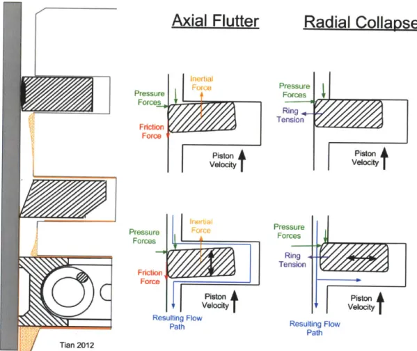
Figure 1-2 shows a sketch for a cut through the piston with the circumferential

vector being the cutting plane's normal vector. The rings are sitting in their respective groove slots on the piston. Since groove dimensions are slightly larger than ring

dimensions, the rings do not have a fixed position inside the groove and can either sit on the upper groove flanks or the lower groove flanks, which is determined by pressure, inertia and friction forces on the ring. Moreover axial fluttering and radial collapse situations can occur where additional flow passages for blowby is created, as shown

Axial Flutter

Radial Collapse

Resulting Flow _{Resulting Flow}

Path _Path

Figure 1-2: Rings sitting in the piston groove and possible instabilities

on the right side of figure 1-2. This work will rather focus on higher load conditions where both cylinder pressure and ring tension are high so that both instabilities are avoided.

1.1.2

Blowby Flow Path in the Piston Ring Pack

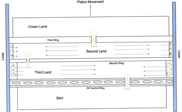
There are 3 main flow regimes for blowby as it passes the ring pack:

" the ring gaps, which are characterized by minimum flow areas, thus choking the

flow,

" the lands between piston and liner in which the blowby has small velocities in

circumferential direction and

Friction Force

Pressure Forces

* the lands in which the blowby is dragged by liner as the piston moves up and down, similar to cavity flows.

A sample sketch of the blowby flow path inside the ring pack is shown in

where gap flows are in orange, circumferential flows are in blue and cavity

in red. Ring Gap flows are mainly characterized by minimum flow areas

Piston Movement

I

-

---

---

I

Figure 1-3: Flow regimes in the ring pack

ring pack which choke the flow during most crank angles.

Circumferential flows in the lands are fairly slow flows due to the total pressure

loss after the ring gaps and the large area expansion. In the second land, the cross sectional flow area normal to circumferential flow direction is 2 orders of magnitues

larger than the gap area, which will cause velocities to drop by 2 orders of magnitude. Cross sectional flows in the lands are cavity types of flows which get dragged by

the liner as the piston moves up and down in the cylinder.

This work investigates each of the 3 types of flows from upstream to downstream, starting at the first ring gap, continuing into the circumferential flow in the second

land and concluding in the third land cross section.

0 C

-1.2

Motivation and Objectives

This work aims at

1. estimating relevant flow parameters

2. developing qualitative and quantitative insight into different flow regimes and

3. couple theoretical findings with high fidelity CFD calculations

This will allow engine designers to understand critical oil transport mechanism to control and reduce oil consumption. At the start of each chapter, a more detailed overview on specific objectives for the respectively discussed flow regime will be given.

1.3

Related Research

Tian et al. [11] estimated gas flow through ring gaps using an isentropic orifice flow relationship

Thgap CDAgappufm

/' R Tu with

fm = V/ (1.2)

7+1

for choked flow and

CD- 0.85 - 0.25PR2

(1.3)

from experimental data (Shapiro [9]), where PR is the downstream to upstream static pressure ratio.

Senzer [8] showed the relationship of drained oil mass flow rate and blowby volume flow rate in the oil control ring (OCR) groove by assuming a parallel separated two-phase flow without mixing. Combining a Poiseuille type of flow for high inertia blowby air and a Couette type of flow for the dragged oil, the mass flow rate relationship of both phases becomes

where 3 represents the non-dimensionalized oil height in the OCR groove 3 . This proportional relationship is in good accordance to measurements carried out in

Chapter 2

Air flow through ring gaps

In chapter 1.1.2 it was stated that the first ring gap is the main mechanism of con-trolling blowby because of the flow choking. The main focus in this chapter lies

in the investigation of geometric and thermophysical parameters on the amount of blowby mass flow with the overall aim for designers to understand and control blowby.

Moreover implications on oil transport are gained by looking at flow patterns at the gap.

2.1

Definition of Test Cases

2.1.1

Choking at the first Ring Gap

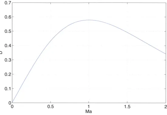
For the choked flow assumption to be true, the corrected flow per unit area

D = t (2.1)

A* ptNfi

which is described in detail by Greitzer et al. [1], must have a global maximum at

the first ring gap, as shown in figure 2-1, where the corrected flow per unit area against Mach number is plotted. The whole ring pack can be simplified to a series

of 3 nozzles, each representing one ring gap, with subsequent sudden expansions as sketched on figure 2-2. For the first nozzle to choke, the condition

0.7

0

0 0.5 1 1.5 2

Ma

Figure 2-1: Corrected Flow per Unit Area

Combustion Chamber and Crown Land Second Land Third Ring Gap Mixing Mixing Losses Losses

0D

Figure 2-2: Ring Pack Simplification

Di > D₂,Di > D3

must hold, or similarly by assuming constant gas values and no heat transfer

D1 pt2A2 D1 pt3A3 -< D D2 -pn A₁' D93 - p1A Exit to Crankcase (2.2) (2.3) Third Land

because rh has to be constant in all 3 nozzles in the steady-state case due to continuity. For very large area ratios at the sudden expansions entropy is generated due to mixing and the resulting stagnation pressure loss is almost as large as the whole dynamic pressure, which has been shown for example by Ward-Smith [12]. That means that the stagnation pressure Pt2 scales as

Pt2 = Pt 2 P (2.4)

and the stagnation pressure ratio scales as

A2 P1 - 1+ Ma2) 7-Y _(2.5)

Pti Pti 2

For Mach numbers in the order of 10-1 and 100 the stagnation pressure ratio Pt2/Pti

typically varies from 0.5 to 1 and pt3/pti varies from 0.25 to 1, whereas both area ratios A2/A1 and A3/A1 are usually always in the order of 5 or larger due to the large

clearances d in subsequent lands. This simple scaling shows that

< 1 < 1 (2.6)

D2 'D 3

and thus choking at the first ring gap always occurs. This has been shown by pressure measurements in the Sloan Automotive Lab as well.

2.1.2

Relevant Geometry

Upper Compression Ring

In the case where friction and inertia push the ring towards the upper flank it is easy to determine the minimum blowby flow area as the gap cross sectional area in axial direction. During combustion, the pressure ratio across the ring is very large and the ring mostly sits on the lower flank of the groove. In this case it becomes unclear where the minimal flow area is and this study will focus on that type of situation. The resulting flow sections inside the groove are outlined in figure 2-3. Typical gap

Groove Wall

Figure 2-3: Possible Flow Path in the Piston Groove

widths L range from 0.2mm to 0.4mm. Here, a gap width of 0.3mm is chosen.

Chamfer and Land Clearance

One of the features of the piston is its chamfer below the first ring, as shown in figure 2-4. Previous experiments and real world cases have indicated that size and shape

Figure 2-4: Piston groove with (right) and without chamfer

The chamfer angle is typically 450 whereas its depth c, as shown in figure 2-5, can vary from engine to engine. Variations in chamfer size from 10pm to 100pm are

carried out in this work to study its effect on blowby. Because the piston can tilt and

Ring Gap

Chamfer

d

_isto

F7X//Land

Figure 2-5: Sketch of the Ring Gap

expand under different thermal conditions than the liner, the clearance between the piston land and the liner can vary during an engine's operating cycle and life. Typical values for the clearance in the second land d range from 100pm to 200pm, for which this study will be conducted.

2.1.3 Computational Domain

The first area in the engine where flow parameters are definitely known is in the combustion chamber, where we can consider the flow at rest with a given total tem-perature T and total pressure pt. This is represented as a classical plenum. Given the overall objective of determining the blowby air flow rate, only the flow at the first ring gap where minimal flow area occurs is of interest because choking limits the mass flow rate, rendering the flow downstream of the choking spot of no interest for this study. The difficulty is the definition of the actual minimum flow area when there is a chamfer below the ring gap. For this reason the domain is extended far away from the ring gap to allow the flow to fully development right after the gap, such that

partial derivatives of flow parameters normal to the boundary Dn disappear to make use of Neumann boundary conditions. The finalized complete computation domain is shown in figure 2-6 that represents a plenum flow out of a converging nozzle into a given atmospheric pressure, which is the static pressure of the piston first land. This plenum flow configuration is further expanded with a groove section as shown on the

right side of figure 2-6.

Figure 2-6: Computational Domain

2.1.4

Relevant Parameters

From compressible flow theory it is known that the air mass flow rate is determined

by gas properties, upstream stagnation values and geometry. In the given cases the

mass flow rate rngap of blowby air with air properties R and -y depends on the plenum stagnation values pt T and the minimum flow area A*, which depends on the two geometric parameters c and d. From dimensional analysis we obtain the two non-dimensional products D and

C

C

where C is a geometric parameter and D is the aforementioned corrected flow per unit area. As previously stated, predicting the choking area A* a priori is very difficulty and thus the area Arej = L-d is used for the choking area. A more thorough discussion on the that area will be given in section 2.3 when results are discussed.

Given the calculation ranges as described in section 2.1.2, this study varies C from

0.05 to 1. To summarize, all test cases for geometric variations are listed in table 2.1

Table 2.1: Geometric Variations for Test Cases

2.1.5

Boundary Conditions

There are 4 different boundary types used in this study:

* The inlet plenum is specified by stationary flow and its stagnation values.

- Since the main idea is to choke the flow, a sufficiently large total to static pressure ratio is chosen to just choke the flow since large pressure ratios will cause an increase in computational residuals. Although absolute mass flow is dependent on pt and T, the previous non-dimensionalization will cause the corrected flow per unit area to be the same maximum value whenever choking occurs and thus should make variations in pt and T unnecessary.

- To verify this non-dimensionalization effect, calculations with variations in the combustion temperature T are conducted for a range from 400K to 2000K and later verified to expected values.

- Setting a fixed value of Om/s caused difficulties in converging the

calcula-tion since it sets a fixed constraint on the flow boundary. At the vicinity of the inlet corner singularity, flow from the top boundary can enter the

c = 10pm c = 40pm c = 70pim c = 100pm

d = 100pm C = 0.1 C = 0.4 C = 0.7 C = 1

d = 150pm C =0.067 C = 0.267 C =0.467 C = 0.667 d = 200ptm C =0.05 C = 0.2 C =0.35 C = 0.5

left inlet boundary and vice versa. This will cause either non-zero veloci-ties and a subsequent crash in the calculation or an artifical creation of a velocity-pressure wave. Both effects are undesired and thus the boundary condition pressureInletOutletVelocity is chosen to allow some backflow at the corner region. For an inflow condition the velocity is obtained using the flux from the first adjacent cell of the boundary.

" As mentioned in section 2.1.3 the outlet is far away so that Neumann boundary

conditions for temperature and velocity hold for the fully developed flow. The pressure is specified as Dirichlet condition to meet the critical pressure ratio. Theoretically, the first law states that the total temperature in the flow field must remain constant because this case does not involve heat or work addition. This implies that setting a Dirichlet condition on the total temperature at the outlet to match inlet and outlet T sets a perfect constraint on the temperature field. In practical usage, this idea is soon discarded because a Dirichlet type of boundary condition sets a very strict constraint on the calculation and slight mistakes by the solver render a full convergence very difficult. Indeed, setting only one dirichlet condition on both pressure sides already causes the case to be difficult to converge.

" For simplification, the effects of heat transfer on choking are taken out by using

adiabatic walls. It can be expected that heat addition would increase the total temperature and thus cause the flow to choke earlier, decreasing the amount of blowby. This effect is already described in detail by Greitzer et al. [1] and could possibly be included in further studies in the future.

" To save computational time, the symmetric ring gap geometry is split in half

with the symmetry boundary condition at the plane of symmetry.

2.1.6

Gas

Properties and Flow Regime

A single phase perfect gas with air properties is chosen as working fluid. For more

re-alistic calculations, fuel-air mixture properties might be more appropriate, especially under heavy load conditions. The gas values are kept constant with dynamic viscosity p = 2.3. 10- 5kg/m - s, Prandtl number Pr = 0.7, heat capacity c, = 1007J/kg - K and specific gas constant R = 287J/kg - K. Using the same non-dimensionalizing argument as for total pressure, these values are kept constant throughout the whole study.

Estimating the Reynolds number inside the combustion chamber UL 1013 - 10-4

Remax-plenum - 2.5 -0-5 102 (2.8)

shows that a laminar flow assumption for the flow inside the combustion chamber is sufficient because flow velocities are in the order of 100 to 101. Close to the gap flow velocities rise to orders of 103m/s to 104m/s and the flow can turn turbulent. On the other hand, there are two important time scales after the flow chokes. The convection time scale gives an idea on how much time is needed for the flow with velocity U to pass the distance D from close to the gap to the outlet

D

10-teonvection U 102 (2.9)

The viscous dissipation time gives an estimation on how long is needed for viscous

Table 2.2: Boundary Conditions

Boundary Pressure [bar] Temperature [K) (U" UY, U_') [m/s] Inlet pt =2.1 Tt = 400 - 2000 pressureInletOutletVelocity

Outlet p =I zeroGradient zeroGr adient

Walls zeroGradient zeroGradient pressureInletOutletVelocity

effects at the walls to be transported within the flow area's hydraulic diameter h

h2 10-5

thAos 10-810-3 (2.10)

Thus the ratio between convection and viscous dissipation time is

tconvection ~ 10 2 (2.11)

tvSCOUS 10-3

This means that even if turbulence is created at the walls when the flow is almost choked, the time needed for turbulence to develop inside the flow field is much larger than the residence time of the flow inside the domain. With this scaling assumption the flow can be safely modeled as laminar to save large amounts of computational resources.

2.1.7

Governing equations and solution method

Generally 4 equations are needed to solve for the 4 unknown variables p, T, p and U in a compressible calculation. As with most solvers, the solver rhoSimplecFoam, which is used here, uses the steady state continuity equation

V - (pU) = 0, (2.12)

the steady-state momentum equation neglecting field forces

pU - VU = -Vp + Vr, (2.13)

the steady state energy equation in enthalpy form without field forces or sources within the fluid

U2

pU - V(h + )=-V +V - (rU) (2.14)

2

and the ideal gas law

where V) is commonly in OpenFOAM defined as

OP=

(2.16)

Source terms are neglected throughout the equations because they are accounted for

in the boundary conditions.

Assuming Newtonian Fluid, the momentum equation can be discretized to

H. 1

Uia- a,1V p

ap ap (2.17)

as shown by Jasak [3], who also defines the quantities H and a, as matrix decompo-sitions from intermediate steps. For better legibility the indices i will be omitted in discretized equations in further equations.

Combining 2.12, 2.17 and 2.15 yields the steady state pressure equation

p

a/ -APP= 0 (2.18)

which is the core of the used rhoSimpleFoam solver. Its SIMPLE algorithm is implemented in OpenFOAM as follows:

1. Initialize, read or create density, pressure, enthalpy, V), velocity and flux fields

2. Guess the velocity field U from solving the momentum equation

3. Guess the density using the ideal gas law

4. Set up and solve the pressure equation, repeat for non-orthogonality

5. Update the velocity- and density fields using the newly calculated pressure

6. Solve the energy equation for enthalpy/temperature

2.2

Total Temperature Fields

Figure 2-7 shows that the total temperature fields still vary after choking but the

errors are around 10% -20% and thus much lower than the total temperature changes in sonicFoam. A closer look at the flow field in figure 2-8 shows that the errors occur

Figure 2-7: Total temperatures for T = 400K (left) and T = 2500K

mostly after choking.

2.3

Blowby flow at the ring gap

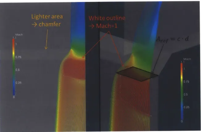
Looking directly at the reference area in figure 2-9, two important observations can be made:

1. Boundary Layers decrease the choking area

2. There is only a small section of flow at Ma =1

Ma

0,25 0 5 O 7 5 3

0 1.22293

Because the Mach-number varies by around 20% from the expected value of Ma = 1 outside the boundary layers, the reference area is not a very good representation of the choking area. The white line in figure 2-9 indicates an isoline for Ma = 1 and the large area on the lower right side of the dividing Ma = 1 isoline indicates unchoked flow. This implies that the real choking area cannot be represented by any flat two dimensional plane and the reference area is only (part of) a projection of the real choking plane.

Figure 2-11 shows that the flow is choking close to the lower end of the chamfer with the approximate reference area of Aref = L - d which is marked as the black

area. As implied by figure 2-9, the real choking area cannot be described in any two dimensional Cartesian room and varies with changes in geometric parameters as in figure 2-10 where contours for Ma = 1 are shown inside the computational domain

for C = 0.02 and C = 1. The flow development after the gap and thus the choking

Figure 2-10: Contours of Ma = 1 for C = 0.2 (left) and C = 1 area is mainly determined by 3 effects:

1. Flow area decrease in piston axial direction due to the chamfer

2. Flow expansion into piston circumferential direction due to pressure gradient

in addition to the boundary layer effect as shown in figure 2-9.

The first effect can be seen on sketch 2-5 and on the right side of figure 2-11. The left side of figure 2-11 shows a view on the plane normal to the radial piston

Figure 2-11: Streamlines through the gap

direction, where we can see the flow expanding into circumferential direction right as it comes out of the ring gap. This effect of flow widening counteracts the decrease in

area throughout the chamfer and thus creates a larger choking area than the a priori

assumed Aef = L -d.

Flow separation at the chamfer can be seen in figure 2-12. If C becomes too small

the flow will separate at the chamfer and thus decrease the total flow area.

2.4

Variations of

C

The corrected flows per unit areas with the a priori assumed choking area Arcf are

plotted in figure 2-13. For values of C larger then 0.3 the corrected flow takes a value larger than the theoretical maximum value of 0.57. This indicates that the

Figure 2-12: Flow separation at the chamfer 0.85 0.8-0.75 x o 0.7 -~ x 8 0.65- 0.6-x x 0.55- x x d=0.lmm d=0.15mm d=0.2mm 0.5' x 0 0.2 0.4 0.6 0.8

Non-dimensionalized chamfer depth C [-]

area used for non-dimensionalization was too small, whereas for values of C smaller than 0.3 the corrected flow indicates a false unchoking of flow, which is due to the non-dimensionalizing area to be too big for that case.

As indicated the flow areas are smaller than the reference area for smaller C where the effect of flow separation at the chamfer is more significant than the flow expansion into circumferential direction. Increasing C keeps the flow better attached to the chamfer by either increase the chamfer length or decreasing the piston-liner distance and thus creating a higher pressure gradient in the radial direction which keeps the flow attached to the piston wall. This results in the flow widening effect gaining more significance over the separation effect and thus effectively increasing the choking area compared to Arcj. Rearranging the corrected flow by using its maximum value 0.57 for choked flow yields the real choking areas

Achoking = rVRTt (2.19)

Dmaxpt f

The computed areas are non-dimensionalized with the previously assumed reference area Aref and plotted in figure 2-14. This relationship can also be fit linearly for the calculation range and yields the relationship

Achoking _{= 0.51C + 0.85 (2.20)}

This relationship can be used to non-dimensionalize the mass flows for variations in total temperature which is shown in figure 2-15. As can be seen, the corrected flow per unit area changes very little throughout the study which confirms that the choking area does not change much with variations in stagnation temperature. The main fluctuations in figure 2-15 come from the curve fit approximation.

2.5

Variations of T

Because this study focuses on the parametric influence on the mass flow rate, the total temperature can be non-dimensionalized with a reference total temperature which is

1.5- 1.4- 1.3- 1.2-.0 1- 0.9-0.8 -0 0.2 0.4 0.6 0.8

Non-dimensionalized chamfer depth C [-]

Figure 2-14: Choking Areas

0.51 1 1 1 1

1 2 3 4 5 6

TtI/Ttef[-|

Figure 2-15: Corrected Flow using Achoking for different geometries 0.6

chosen as the lowest stagnation temperature case of Tref = 400K. Similarly the mass flow rate can be non-dimensionalized using the mass flow rate of the reference case with a total temperature of 400K. Alternatively non-dimensionalizing the mass flow to the corrected flow per unit area is another option, which is more difficult due to the lack of a minimal choking area.

The relationship between absolute mass flow rate and stagnation temperature can be calculated, starting with the absolute mass flow which given as

rh= p*c*Aehoking (2.21)

where p* and c* can be calculated with the isentropic flow relationships

1 P Pt

(1

Plugging in Ma = 1 into (2.22) and (2.24) yields 1

c* =7RT (i1 + 7 1 Plugging (2.25), (2.26) and the ideal gas law

pt RT (2.22) (2.23) (2.24) (2.25) (2.26) (2.27)

into (2.21) gives the relationship

+-y 3

rh = 1 + 7 1 2 ( -) N/VAchoking

V/ T, 2

(2.28)

Using the choking area relationship from (2.20) yields the relationship between ab-solute mass flow and stagnation temperature, which is plotted against calculation

values in figure 2-16. This comparison shows good agreement between CFD results

1.1

2 3 4 5

Tt/Ttref[ _]

Figure 2-16: Analytical Comparison for Mass Flow Rates

and analytically expected values with a maximum error of 6% for the reasonable range

of stagnation temperatures.

Another interesting observation is the wake behavior that is indicated in figure

2-17. Although the calculation has a 10% error in total temperature in the wake, the

qualitative behavior shows that the vortex intensifies and becomes larger as the total

temperature is increased. This causes higher mixing losses and results in a faster drop in pt which causes D to raise and thus unchoke the flow earlier as seen in figure 2-18. Since the geometry does not change in the parametric study for T the maximum

Figure 2-17: Velocity vectors for T - 400K (left) and T - 2500K

Figure 2-18: Mach numbers for T = _{400K (left) and T = 2500K}

magnitude of U, at the boundary layer border is increased while the distance into y-direction remains unchanged, creating a larger velocity gradient and thus larger vorticity, as shown in figure 2-19. Lines with same color refer to velocity profiles at same locations for T = 400K and T = 2500K. Different colors indicate locations of 0.2mm, 0.3mm, 0.4mm and 0.5mm distance from the gap, where higher velocities occur at positions closer to the gap. The exact mechanisc of vortex creation will be

X 10~4 1.51r 0.5- _{- - - 2500K} 0/ / III 0 50 100 150 200 250 300 U [m/s]

Figure 2-19: Velocity profiles close to the gap

described in more detail in chapter 3.

2.6

Comparison to Previous Results

Tian et al. [11] derived a choking area relationship as

Aehoking = CD Agap where Agap = L(d+f -c) CD = 0.85 - 0.25 2 PD (Pu)2

The chamfer factor

f

350

(2.29)

(2.30)

coefficient of CD= 0.8. This yields the relationship for the average choking area

Achoking= 0.8L (d + 0.6c) (2.32)

The simulated choking area given in (2.20) can be slightly rearranged to

Achoking= 0.85L (d + 0.6c) (2.33)

which represents a 6% larger choking area than in experimental measurements. The most likely reason for this discrepancy lies in the omitting of heat transfer during the calculations. As mentioned in figure 2-1 it can be seen that in the subsonic case the corrected flow per unit area is increasing until choking occurs and then decreases again in the supersonic flow region. Heat transfer will raise the total temperature in the flow and will thus increase D and the flow Mach number in the subsonic region, causing the flow to choke earlier at a smaller area. For a more complete calculation heat transfer should be implemented, but there will be additional difficulties in defining a suitable test case because of the non-uniform piston and liner temperatures and the lack of a clear heat transfer area. As seen in figure 2-17, the blowby air is coming from all the groove and combustion chamber. In a real case this air will already be pre-heated to a certain total temperature based on its travel distance before entering the computational domain. Two options to account for the heat transfer inside the combustion chamber are to analytically develop a better total temperature approximation at the boundaries or extending the domain to the full geometry. Neither option is feasible given the resources and time in this work, but could be included in further studies to drive down the 6% error.

2.7

Implications on Oil Transport

Following the discussion of Senzer [8], the amount of oil transport inside the OCR groove can be directly controlled with the amount of blowby. This study shows that the geometric parameters downstream of the gap outlet still play a role in determining

the choking area and thus the blowby mass flow rate. Designers can thus focus on ring outlet and chamfer geometries to increase or restrict blowby. Decreasing blowby

can be achieved by

" Removing possible chamfers from ring and piston

* Decreasing chamfer size c, piston-land clearance d or gap size L

" Change chamfer angle to choke earlier, giving less time for circumferential

ex-pansion and thus decreasing choking area

" Sharpen corners to facilitate flow separation

The implications for oil transport that are gained in the studying of blowby are

" Higher combustion temperatures lead to larger oil accumulation areas below the

gap

* Oil from the combustion chamber is more likely to be convected by air flow to

the second ring groove if the combustion temperature is lower

* Mixing losses increase as stagnation temperature rises, possibly unchoking the first gap for very high combustion temperatures which would cause an even larger decrease in blowby mass flow

" Smoother flow without separation lead to less areas with no flow and thus less

places where oil can sit without being convected by air. Separation and vortices

Chapter 3

2nd land air flow

The main goal in this chapter is to understand where possible oil accumulation areas are and where oil is likely to be convected by blowby. The groove and variations of gap posisions are included to study resulting flow paths and to understand where oil

can possibly be transported into and out of the groove.

3.1

Definition of Test Cases

3.1.1

Steady choked condition

The calculations are run in steady state with a choked flow inlet. A first transient calculation is conducted to investigate transient effects, for example gas compression and waves, to understand the time it takes to choke the flow after the critical pressure ratio is achieved. For that purpose, the transient total to static pressure ratio from experimental measurements is imposed as boundary condition. Figure 3-1 shows the pressure ratio and Mach number evolution in time. After a short instable calculation phase of rougly 30 crank angles the Mach number at the inlet follow the same trend as the pressure ratio and hits the choking value 1 only 2 crank agles after the critical pressure ratio of 1.89 is reached. This leads to the conlusion that the choked flow inlet condition is suitable and thus higher pressure ratios will only have an effect on absolute mass flow.

2-E

z

1

Pressure Ratio

Inlet Mach number -360 -340 -320 -300 -280 -260 -240 -220 -200

CA

Figure 3-1: Inlet Mach number and pressure ratio

3.1.2

Computational domain

The calculation focuses on the rings being on the lower groove flank conditions, as mentioned in section 1.1.1 with a resulting flow path in the groove as outlined in section 2.1.2. Because the inlet has been determined as choked, a small area in the land's top area can represent the inlet gap. The land itself is either modeled as symmetric half-circle if gaps are exactly opposite or with whole circumferential length for the study of gap positional effects. To reduce exit boundary influences on the flow inside the second land, the computational domain is extended into the third land again using a Neumann type of boundary condition for fully developed flow. Preliminary boundary condition studies showed that velocity waves still existed and influenced the flow pattern at the exit ring gap. For this purpose, the non reflecting exit boundary condition waveTransmissive is chosen, which is described by Poinsot et al. [6]. The resulting symmetric domain is shown in figure 3-2. Non-symmetrical cases vary only the inlet and outlet positions and the inclusion of the other half of the land.

Figure 3-2: Computational domain for land calculations

3.1.3

Boundary conditions

This study uses 4 different boundary types:

* The choked gap inlet is specified by exit static pressure, the measured piston temperature of Tiniet = 423.15K and the choked flow velocity which is calculated

from Uiniet = Cinlet =yVRTinlet

" The outlet is far away so that Neumann boundary conditions for temperature

and velocity hold for the fully developed flow. The pressure is set from

exper-imental measurements for an early compression stroke where static pressures

at the inlet and at the outlet are similar. Having a lower back pressure would result in a choking of the third gap as well due to higher losses in the second land. This back pressure effect could be investigated in future studies

" Heat transfer effects are again neglected by the usage of adiabatic walls

* (The whole circular land is split into two symmetrical halfes in the case of

exactly opposing gaps)

3.1.4

Governing equations and solution method

The governing equations are the same as outlined in section 2.1.7. For the transient

calculation, the only difference are included time derivative terms, which lead to a transient pressure equation of

00_

((H"\1)

±V* -0p- -A =0 (3.1)

3.2

Oil accumulation at the inlet gap

The main accumulation area for oil is inside blowby vortices where the low pressure cores can suck and trap oil inside. The intensities and sizes of the vortices vary

with total temperature as seen in section 2.5 and can be explained from a vorticity

standpoint using a 2D simplification. At the walls before the inlet gap, vorticity is created in the boundary layers and convected with the flow. After passing the sudden

expansion, the boundary layer vorticity that is carried by the fluid causes streamline curvature into circumferential direction and thus creates the vortex as sketched on

figure 3-3.

For higher stagnation temperatures the amount of vorticity created in the

bound-ary layers increase due to a larger velocity gradient. The z-component of vorticity is defined as

W, =

au"

Ox Oy

Using the simplified sketch in figure 3-3 assuming parallel flow, the component O

is 0 and the vorticity describes the clockwise rotation rate of the drawn material line. The same conclusion can be achieved from pressure arguments. Because of

Table 3.1: Boundary Conditions

Boundary Pressure [bar] Temperature [K) (U.,, Uy, U,) [m/s] Inlet p = 1 T = 423.15 (0, -412.34, 0)

Outlet p = 1 zeroGradient wavetransmissive

Walls zeroGradient zeroGradient (0,0,0)

Figure 3-3: Vorticity at sudden expansion

Mach-number similarity throughout variations in total temperature the pressure field

is roughly similar based on

- Ma 2 7-Y

2 (3.3)

p

+

but the velocities inside the groove scale as

U ~ c ~ VIT ~ T

For vortices, pressure and velocities follow the relationship

U2 Op p- = r Or (3.4) (3.5)

as outlined by Lord Rayleigh [7]. Having similar pressure fields but larger velocities for higher stagnation temperatures means the vortical radius increases for growing

stagnation temperatures.

Another factor on vortex forming that was not included in chapter 2 comes from

presence of the second ring. The incoming air stream is slowed down at the second

ring wall and creates a stagnation point with high stagnation pressure. This will cause two main pressure gradients to arise:

1. At the second ring, the high stagnation point causes a pressure gradient in

circumferential and axial direction pushing the flow away from the stagnation

point. This will result in a large vortex inside the land on both sides of the inlet

ring gap.

2. Between the ring gap and the stagnation point, expansion causes a pressure drops until the flow unchokes due to mixing losses. These local low pressure

regions form smaller vortices, which are unsteady and conveted with the flow. The unsteadyness arises from the asymmetry of the expansion, except in the case

where gaps are exactly opposite. Pressure gradients into both circumferential directions are different and thus a tendency towards the higher accelerating

direction forces the first secondary vortex into that direction. This leads to a dead space region and subsequent low pressure region on the other side, which

will form another vortex and vice versa.

The resulting pressure field and vortices are shown in figure 3-4. There are two main areas where vortices form in a ring down position:

" In the land below the inlet ring gap, as already discussed in chapter 2

" Inside the groove below the the inlet ring gap.

Figure 3-5 shows experimental indicators for the accumulation of oil on both sides be-low the inlet gap as predicted by the simulated vortices. White areas represent regions

of oil accumulation where higher brightness indicates a thicker oil film. Moreover fig-ure 3-6 indicates the unsteady shedding of vortices. One difference in figfig-ure 3-6 is

Figure 3-4: Pressure field and velocity vectors below the inlet gap inside the land

Figure 3-5: Experimental measurement of oil puddles below the first ring gap

the reversed flow direction which implies that the insights gained in this study can be reversed in direction for intake and expansion strokes. After the blowby air reaches the second ring, a part enters the groove due to the high pressure stagnation point on the second ring, as sketched on figure 3-7. The high inertia air flow creates another

Figure 3-6: Puddle shedding due to unsteady vortices

Figure 3-7: Pressure field and velocity vectors below the inlet gap inside the groove flank

vortex in the groove due to the same mechanisms as the vortices below the inlet ring gap, which can be seen in figure 3-8. This causes oil accumulation inside the groove below the ring gap. As oil puddles form within the ring groove, ring movement can

Figure 3-8: Streamlines showing vortices in the second ring groove

push oil out of the groove into the neighboring land, as shown in figure 3-9.

Figure 3-9: Oil puddles in the crown land, pumped back after accumulatin in first rign groove

3.3

Air flow far away from the gaps

Flow velocities inside the land can be estimated using continuity. Depending on the relative position of the gaps, mass flow from the inlet distributes into both

circum-ferential directions differently. The necessary assumptions area

* The flow inside the lands are laminar, based on a scaling which shows that UD 10010-3

Rb= =102

v10-5 (3.6)

which is clearly below the turbulent onset

. The flow inside the lands is fully developed, which given for the condition that

RD (D)2

L «1 (3.7)

* The entry length is very short compared to the whole circumference. This can be estimated for laminar flow with

Lentry _{= 0.06ReD}

(D)

(10-1) (3.8)

as outlined by Kundu [4].

This simplifies the Navier-Stokes equation in circumferential direction to

0 2 Utheta

Or2

OP

0g (3.9)

Solving the resulting Poiseuille type of flow yields a proportional relationship between velocity in the lands and the pressure gradient. The ratio of flow into the close direction, which is the circumferential direction into which the distance between inlet and outlet gap is shorter, and flow into the far direction M thus scale directly with

the ratio of their pressure gradients. (p M = elose ~ 9/ close mfar 001/ far (3.10)

This can be seen in figure 3-10 where mass flow rates from several calculations with

different gap positions are compared to the analytical relationship. The deviation

0 _0 E

27r

Nt

Circumferential position [rad]

Figure 3-10: Ratio of mass flows for different gap positions

from analytical results as the gaps move closer to each other are due to the shortened

time for flow development which causes the fully developed flow assumption to be less accurate.

Drawing a control volume as sketched in figure 3-11, where the flow is fully

devel-oped at the land border, the mass flow into the close direction is

mclose + rnfar m _{o ~far} 1±+ mciose minlet 1 + M (3.11)

Second ring

Figure 3-11: Control volume in the second land

The velocity ratio between inlet and close direction outlet can be estimated as

PcioseUciose Aclose (1 + M) = PinietUinletAinlet (3.12)

which can be rearranged to

Uciose _ 1 _{Pinlet Ainet}

3.13) Uiniet 1 + M pelose Aciose

The density ratio can be estimated using an isentropic flow relationship which slightly underpredicts the value of Pciose

Pinlet 1 +2 close ₍₃₁₄₎

Pciose 1 + 2Y1M _{2 inlet}e

where the inlet Mach number is 1, giving density ratios Pinlet/pciose of 1.36 to 1.58 for

Maciose being between 0 and 0.3. The area ratio Ainiet/Acose is around 0.02. This leads to velocity ratios in the order of

Uciose 10-2 _(3.15)

Uiniet

The analysis used a single cross sectional area for the land until now, which can be further divided into land and groove area. In equation 3.9, the pressure gradient is

the same in both groove and land but the radial dimension is one order of magnitude

larger in the groove than in the lands. Flow velocities in the lands are thus an order of magnitude less than in the groove. The scaling analysis has given two important conclusions about air flow far away from the gaps:

" Flow velocities in the groove are one order of magnitude higher than in the

lands

" Flow velocities in the groove are two orders of magnitude lower than at the inlet

This can be seen in the flow cross section on figure 3-12, where the inlet velocity is

close to 400m/s. Comparing the shear forces from the air which scale as pU/hflank

Figure 3-12: Velocity magnitudes in the land and in the groove

with the capillary stresses of oil inside the groove which scale as o-hfilank yields the Capillary number U 'tan pU 10-510-2 Ca l - = 10 hf- 10-hf lank (3.16)

The small Capillary number indicates that in most of the land areas, shear effects on oil can be mostly neglected and oil that is far away from either gap is not influenced

3.4

Blowby at the outlet gap

The pressure drop from the upstream influence of the outlet ring gap causes the flow to accelerate. This will cause flow from the land to enter the groove due to its lowered resistance, as mentioned in section 3.2. The extend of upstream influence can be estimated using disturbance theory as outlined by Greitzer et al. [1].

Assuming irrotational incompressible flow upstream up the gap, it can be shown that the upstream influence of the gap pressure disturbance p' satisfies the Laplace equation

Ap - + + (3.17)

Ox2 0

_y

_Oz

The lack of an intrinsic length scale implies that if a length scale in one direction is set, the length scale in the other directions take the same magnitude. In this case, a length scale set by the geometry is the gap opening. As seen in figure 3-13, only area within one gap opening distance to the gap is influenced by the gap. Because

Figure 3-13: Upstream influence of the outlet gap and distance until flow is fully developed

large velocities only occur close to the gap, only oil in the vicinity of the gap will be transported away. This means that it is favorable to have the gap close to areas of large oil accumulation. Examples where this plays a role are

" Large oil puddles from non-conforming oil control rings on the liner

" Leaking areas on the liner

" Oil puddles inside the groove that can be pumped into the second land by the

second ring

Equation (3.16) showed that surface tension of oil is dominant compared to shear

if velocities are below the order of 102m/s. This only happens after the upstream

influence of the outlet gap has increased flow velocities and thus the dragging of oil only becomes significant at the gap itself.

3.5

Conclusion on 2nd land air flows

The whole flow path is shown in figure 3-14 and the main conclusions for oil transport

Figure 3-14: Streamlines showing the whole flow path inside the second land and second ring groove