HAL Id: hal-02154306
https://hal.archives-ouvertes.fr/hal-02154306
Submitted on 18 Dec 2019
HAL is a multi-disciplinary open access
archive for the deposit and dissemination of
sci-entific research documents, whether they are
pub-lished or not. The documents may come from
teaching and research institutions in France or
abroad, or from public or private research centers.
L’archive ouverte pluridisciplinaire HAL, est
destinée au dépôt et à la diffusion de documents
scientifiques de niveau recherche, publiés ou non,
émanant des établissements d’enseignement et de
recherche français ou étrangers, des laboratoires
publics ou privés.
Riccardo Dondi, Manuel Lafond, Celine Scornavacca
To cite this version:
Riccardo Dondi, Manuel Lafond, Celine Scornavacca.
Reconciling multiple genes trees via
seg-mental duplications and losses. Algorithms for Molecular Biology, BioMed Central, 2019, 14 (1),
�10.1186/s13015-019-0139-6�. �hal-02154306�
Riccardo Dondi
, Manuel Lafond
and Celine Scornavacca
Abstract
Reconciling gene trees with a species tree is a fundamental problem to understand the evolution of gene families. Many existing approaches reconcile each gene tree independently. However, it is well-known that the evolution of gene families is interconnected. In this paper, we extend a previous approach to reconcile a set of gene trees with a species tree based on segmental macro-evolutionary events, where segmental duplication events and losses are associated with cost δ and , respectively. We show that the problem is polynomial-time solvable when δ ≤ (via LCA-mapping), while if δ > the problem is NP-hard, even when = 0 and a single gene tree is given, solving a long standing open problem on the complexity of multi-gene reconciliation. On the positive side, we give a fixed-param-eter algorithm for the problem, where the paramfixed-param-eters are δ/ and the number d of segmental duplications, of time complexity O ⌈δ
⌉ d
· n ·δ . Finally, we demonstrate the usefulness of this algorithm on two previously studied real datasets: we first show that our method can be used to confirm or raise doubt on hypothetical segmental duplica-tions on a set of 16 eukaryotes, then show how we can detect whole genome duplicaduplica-tions in yeast genomes.
Keywords: Phylogenetics, Gene trees, Species trees, Reconciliation, Segmental duplications, Fixed-parameter
tractability, NP-hardness, Whole genome duplications
© The Author(s) 2019. This article is distributed under the terms of the Creative Commons Attribution 4.0 International License (http://creat iveco mmons .org/licen ses/by/4.0/), which permits unrestricted use, distribution, and reproduction in any medium, provided you give appropriate credit to the original author(s) and the source, provide a link to the Creative Commons license, and indicate if changes were made. The Creative Commons Public Domain Dedication waiver (http://creat iveco mmons .org/ publi cdoma in/zero/1.0/) applies to the data made available in this article, unless otherwise stated.
Introduction
It is nowadays well established that the evolution of a gene family can differ from that of the species contain-ing these genes. This can be due to quite a number of different reasons, including gene duplication, gene loss, horizontal gene transfer or incomplete lineage sorting, to only name a few [22]. While this discongruity between the gene phylogenies (the gene trees) and the species phylogeny (the species tree) complicates the process of reconstructing the latter from the former , every cloud has a silver lining: “plunging” gene trees into the species tree and analyzing the differences between these topolo-gies, one can infer the macro-evolutionary events that shaped gene evolution. This is the rationale behind the
species tree-gene tree reconciliation, a concept introduced
in [13] and first formally defined in [24]. Understand-ing these macro-evolutionary events allows us to better
understand the mechanisms of evolution with applica-tions ranging from orthology detection [9, 18, 19, 30] to ancestral genome reconstruction [11], and recently in dating phylogenies [5, 7].
It is well-known that the evolution of gene families is interconnected. However, in current pipelines, each gene tree is reconciled independently with the species tree, even when posterior to the reconciliation phase the genes are considered as related, e.g. [11]. A more pertinent approach would be to reconcile the set of gene trees at once and consider segmental macro-evolutionary events, i.e. events that concern a chromosome segment instead of a single gene.
Some work has been done in the past to model seg-mental gene duplications and three models have been considered: the ec (Episode Clustering) problem, the me (Minimum Episodes) problem [1, 14], and the mgd
(Mul-tiple Gene Duplication) problem [12]. The ec and mgd problems both aim at clustering duplications together by minimizing the number of locations in the species tree where at least one duplication occurred, with the addi-tional requirement that a cluster cannot contain two gene
*Correspondence: [email protected] 2 Department of Computer Science, Universitè de Sherbrooke, Sherbrooke, Canada
duplications from a same gene tree in the mgd problem. The me problem is more biologically-relevant, because it aims at minimizing the actual number of segmental duplications (more details in "Reconciliation with seg-mental duplications" section). Most of the exact solutions proposed for the me problem [1, 20, 26] deal with a con-strained version, since the possible mappings of a gene tree node are limited to given intervals, see for example [1, Def. 2.4]. In [26], a simple O∗(2k) time algorithm is
presented for the unconstrained version (here O∗ hides
polynomial factors), where k is the number of speciation nodes that have descending duplications under the LCA-mapping. This shows that the problem is fixed-parameter tractable (FPT) in k. But since the LCA-mapping maxi-mizes the number of speciation nodes, there is no reason to believe that k is a small parameter, and so more prac-tical FPT algorithms are needed. Recently, Delabre et al. [8] studied the problem of reconstructing the evolution of syntenic blocks. Their model allows segmental dupli-cations, but is more constrained since it requires every gene family of every block to have evolved along the same tree.
In this paper, we extend the unconstrained ME model to gene losses and provide a variety of new algorithmic results. We allow weighing segmental duplication events and loss events by separate costs δ and , respectively. We show that if δ ≤ , then an optimal reconciliation can be obtained by reconciling each gene tree separately under the usual LCA-mapping, even in the context of segmen-tal duplications. On the other hand, we show that if δ > and both costs are given, reconciling a set of gene trees while minimizing segmental gene duplications and gene losses is NP-hard. The hardness also holds in the particu-lar case that we ignore losses, i.e. when = 0 . This solves a long standing open question on the complexity of the reconciliation problem under this model (in [1], the authors already said “it would be interesting to extend the
[...] model of Guigó et al. (1996) by relaxing the constraints on the possible locations of gene duplications on the spe-cies tree”. The question is stated as still open in [26]). The hardness holds also when only a single gene tree is given. On the positive side, we describe an algorithm that is practical when δ and are not too far apart. More precisely, we show that multi-gene tree reconciliation is fixed-parameter tractable in the ratio δ/ and the number
d of segmental duplications, and can be solved in time
O ⌈δ ⌉d·n ·
δ
. The algorithm has been implemented and tested and is freely available1 at https ://githu b.com/
AEVO-lab/MultR ec. We first evaluate the potential of
multi-gene reconciliation on a set of 16 eukaryotes, and show that our method can find scenarios with less dupli-cations than other approaches. While some previously identified segmental duplications are confirmed by our results, it casts some doubt on others as they do not occur in our optimal scenarios. We then show how the algorithm can be used to detect whole genome duplica-tions in yeast genomes. Further work includes incorpo-rating in the model segmental gene losses and segmental horizontal gene transfers, with a similar flavor than the heuristic method discussed in [10].
Preliminaries
Basic notions
For our purposes, a rooted phylogenetic tree T = (V (T ), E(T )) is an oriented tree, where V(T) is the set of nodes, E(T) is the set of arcs, all oriented away from r(T), the root. Unless stated otherwise, all trees in this paper are rooted phylogenetic trees. A
for-est F = (V (F), E(F)) is a directed graph in which every
connected component is a tree. Denote by t(F) the set of trees of F that are formed by its connected components. Note that a tree is itself a forest. In what follows, we shall extend the usual terminology on trees to forests.
For an arc (x, y) of F, we call x the parent of y, and y a
child of x. If there exists a path that starts at x and ends
at y, then x is an ancestor of y and y is a descendant of x. We say y is a proper descendant of x if y �= x , and then
x is a proper ancestor of y. This defines a partial order
denoted by y ≤F x , and y <F x if x �= y (we may omit the
F subscript if clear from the context). If none of x ≤ y and
y ≤ x holds, then x and y are incomparable. The set of children of x is denoted ch(x) and its parent x is denoted
par(x) [which is defined to be x if x itself is a root of a
tree in t(F)]. For some integer k ≥ 0 , we define park(x)
as the k-th parent of x. Formally, par0(x) = par(x) and
park(x) = par(park−1(x)) for k > 0 . The number of chil-dren |ch(x)| of x is called the out-degree of x. Nodes with no children are leaves, all others are internal nodes. The set of leaves of a tree F is denoted by L(F). The leaves of
F are bijectively labeled by a set L(F) of labels. A forest is binary if |ch(x)| = 2 for all internal nodes x. Given a set of
nodes X that belong to the same tree T ∈ t(F) , the lowest
common ancestor of X, denoted LCAF(X) , is the node z
that satisfies x ≤ z for all x ∈ X and such that no child of
z satisfies this property. We leave LCAF(X) undefined if
no such node exists (when elements of X belong to dif-ferent trees of t(F)). We may write LCAF(x, y) instead of
LCAF({x, y}) . The height of a forest F, denoted h(F), is the
number of nodes of a longest directed path from a root to a leaf in a tree of F (note that the height is sometimes defined as the number of arcs on such a path—here we
1 To our knowledge, this is the first publicly available reconciliation software
cies tree. Here G can be thought of as a set of gene trees. Each leaf of G represents a distinct extant gene, and G and S are related by a function s : L(G) → L(S) , which means that each extant gene belongs to an extant species. Note that s does not have to be injective (in particular, several genes from a same gene tree G of G can belong to the same species) or surjective (some species may not contain any gene of G ). Given G and S, we will implicitly assume the existence of the function s.
In a DL reconciliation, each node of G is associated to a node of S and an event—a speciation ( S ), a duplica-tion ( D ) or a contemporary event ( C)—under some con-straints. A contemporary event C associates a leaf u of G with a leaf x of S such that s(u) = x . A speciation in a node u of G is constrained to the existence of two sepa-rated paths from the mapping of u to the mappings of its two children, while the only constraint given by a dupli-cation event is that evolution of G cannot go back in time. More formally:
Definition 1 (Reconciliation) Given a gene forest G
and a species tree S, a reconciliation between G and
S is a function α that maps each node u of G to a pair
(αr(u), αe(u)) where αr(u) is a node of V(S) and αe(u) is
an event of type S, D or C , such that:
1 if u is a leaf of G , then αe(u) = C and αr(u) = s(u);
2 if u is an internal node of G with children u1, u2 , then
exactly one of following cases holds:
• αe(u) = S , αr(u) = LCAS(αr(u1), αr(u2)) and
αr(u1), αr(u2) are incomparable;
• αe(u) = D , αr(u1) ≤ αr(u) and αr(u2) ≤ αr(u)
Note that if G consists of one tree, this definition coin-cides with the usual one given in the literature (first for-mally defined in [24]). We say that α is an LCA-mapping if, for each internal node u ∈ V (G) with children u1, u2 ,
αr(u) = LCAS(αr(u1), αr(u2)) . Note that there may be
more than one LCA-mapping, since the S and D events on internal nodes can vary. The number of duplications of α , denoted by d(α) is the number of nodes u of G such that αe(u) = D . For counting the losses, first define for
y ≤ x the distance dist(x, y) as the number of arcs on the
dist(αr(u), αr(u2)).
The number of losses of a reconciliation α , denoted by l(α) , is the sum of lα(·) for all internal nodes of G . The
usual cost of α , denoted by cost(α) , is d(α) · δ + l(α) · [21], where δ and are respectively the cost of a dupli-cation and a loss event (it is usually assumed that speciations do not incur cost). A most parsimonious
rec-onciliation, or MPR, is a reconciliation α of minimum
cost. It is not hard to see that finding such an α can be achieved by computing a MPR for each tree in t(G) sepa-rately. This MPR is the unique LCA-mapping α in which αe(u) = S whenever it is allowed according to
Defini-tion 1 [3].
Reconciliation with segmental duplications
Given a reconciliation α for G in S, and given s ∈ V (S) , write D(G, α, s) = {u ∈ V (G) : αe(u) = D and αr(u) = s}
for the set of duplications of G mapped to s. We define G[α, s] to be the subgraph of G induced by the nodes in D(G, α, s) . Note that G[α, s] is a forest.
Here we want to tackle the problem of reconciling sev-eral gene trees at the same time and counting segmental duplications only once. Given a set of duplications nodes D ∈ V (G) occurring in a given node s of the species tree, it is easy to see that the minimum number of segmental duplications associated with s is the minimal number of parts in a partition of D in which each part does not con-tain comparable nodes. See Fig. 1(4) for an example. This number coincides [1] with hα(s) := h(G[α, s]) , i.e. the
height of the forest of the duplications in s. Now, denote ˆ
d(α) =
s∈V (S)hα(s) . For instance in Fig. 1, under the
mapping µ in (2), we have ˆd(µ) = 6 , because hµ(s) =1
for s ∈ {A, B, C, E} and hµ(F ) =2 . But under the
map-ping α in (3), ˆd(α) = 4 , since hα(A) =1 and hα(F ) =3 .
Note that this does not consider losses though—the α mapping has more losses than µ.
The cost of α is costSD(G, S, α) = δ · ˆd(α) + · l(α) . If G
and S are unambiguous, we may write costSD(α) . We have
the following problem:
Problem 1 Most parsimonious reconciliation of a set of
Instance: a species tree S, a gene forest G , costs δ for
dupli-cations and for losses.
Output: a reconciliation α of G in S such that
costSD(G, S, α) is minimum.
Note that, when = 0 , costSD coincides with the
unconstrained ME score defined in [26] (where it is called
ME under the FHS model).
Properties of multi‑gene reconciliations
We finish this section with some additional terminology and general properties of multi-gene reconciliations that will be useful throughout the paper. The next basic result states that in a reconciliation α , we should set the events of internal nodes to S whenever it is allowed.
Lemma 1 Let α be a reconciliation for G in S, and
let u ∈ V (G) such that αe(u) = D . Let α′ be identical
to α , with the exception that α′
e(u) = S , and suppose
that α′ satisfies the requirements of Definition 1. Then
costSD(α′) ≤costSD(α).
Proof Observe that changing αe(u) from D to S
can-not increase ˆd(α) . Moreover, as dist(α′
r(u), αr′(u1)) and
dist(αr′(u), αr′(u2)) are the same as in α for the two
chil-dren u1 and u2 of u, by definition of duplications and
losses this decreases the number of losses by 2. Thus costSD(α′) ≤costSD(α) , and this inequality is strict when
> 0 .
Since we are looking for a most parsimonious rec-onciliation, by Lemma 1 we may assume that for an internal node u ∈ V (G) , αe(u) = S whenever allowed,
and αe(u) = D otherwise. Therefore, αe(u) is implicitly
defined by the αr mapping. To alleviate notation, we will
treat α as simply as a mapping from V (G) to V(S) and thus write α(u) instead of αr(u) . We will assume that
the events αe(u) can be deduced from this mapping α by
Lemma 1.
Therefore, treating α as a mapping, we will say that α is valid if for every v ∈ V (G) , α(v) ≥ α(v′) for all descendants v′ of v. We denote by α[v → s] the mapping
obtained from α by remapping v ∈ V (G) to s ∈ V (S) , i.e. α[v → s](w) = α(w) for every w ∈ V (G) \ {v} , and α[v → s](v) = s . Since we are assuming that S and D events can be deduced from α , the LCA-mapping is now unique: we denote by µ : V (G) → V (S) the LCA-mapping, defined as µ(v) = s(v) if v ∈ L(G) , and other-wise µ(v) = LCAS(µ(v1), µ(v2)) , where v1 and v2 are the
children of v. Note that for any valid reconciliation α , we have α(v) ≥ µ(v) for all v ∈ V (G) . We also have the following, which will be useful to establish our results.
Lemma 2 Let α be a mapping from G to S. If
α(v) > µ(v) , then v is a D node under α.
Proof Let v1 and v2 be the two children of v. If
α(v) �= LCAS(α(v1), α(v2)) , then v must be a
duplica-tion, by the definition of S events. The same holds if α(v1) and α(v2) are not incomparable. Thus assume
α(v) = LCAS(α(v1), α(v2)) > µ(v) and that α(v1) and
α(v2) are incomparable. This implies that one of α(v1)
or α(v2) is incomparable with µ(v) , say α(v1) w.l.o.g.
But µ(v1) ≤ α(v1) , implying that µ(v1) is also
incom-parable with µ(v) , a contradiction to the definition of
µ =LCAS(µ(v1), µ(v2)) .
Lemma 3 Let α be a mapping from G to S, and let
v ∈ V (G) . Suppose that there is some proper descendant v′
of v such that α(v′) ≥ µ(v) . Then v is a duplication under
α.
Proof If α(v) = µ(v) , we get µ(v) ≤ α(v′) ≤ α(v) = µ(v) ,
and so α(v′) = µ(v) . We must then have α(v′′) = µ(v) for
every node v′′ on the path between v′ and v. In particular, v
has a child v1 with α(v) = α(v1) and thus v is a duplication.
If instead α(v) > µ(v) , then v is a duplication by Lemma 2.
Fig. 1 (1) A species tree S. (2) A gene forest G with two gene trees reconciled under the MPR that we denote µ . The nodes are labeled by the same name of the species they are mapped to but in lowercase. Black squares indicate duplication nodes. Losses are not shown. (3) The same forest G but with another reconciliation α for the internal nodes. (4) The forest G[α,f ] , along with a partition into (possible) segmental duplications
The Shift-down lemma will prove very useful to argue that we should shift mappings of duplications down when possible, as it saves losses (see Fig. 2). For future reference, do note however that this may increase the height of some duplication forest G[α, s].
Lemma 4 (Shift-down lemma) Let α be a mapping from
G to S, let v ∈ V (G) , let s ∈ V (S) and k > 0 be such that park(s) = α(v) . Suppose that α[v → s] is a valid
map-ping. Then l(α[v → s]) ≤ l(α) − k.
Proof Let v1 and v2 be the children of v, and denote
t := α(v), t1:=α(v1) and t2:=α(v2) . Moreover denote
α′:=α[v → s] . Let P be the set of nodes that appear
on the path between s and t, excluding s but including t (note that s is a proper descendant of t but an ancestor of both t1 and t2 , by the validity of α′ ). For instance in Fig. 2,
P = {x, t} . Observe that |P| = k . Under α , there is a loss for each node of P on both the (v, v1) and (v, v2) branches.
(noting that v is a duplication by Lemma 2). These 2k losses are not present under α′ . On the other hand, there
are at most k losses that are present under α′ but not
under α , which consist of one loss for each node of P on the (par(v), v) branch (in the case that v is not the root of its tree—otherwise, no such loss occurs). This proves that
l(α′) ≤l(α) − k .
A “proof-by-picture” of the above Lemma appears in Fig. 2. When shifting down the mapping of v, some losses that appear left and right of v get “combined” on the branch above it.
The computational complexity of the mprst‑sd problem
We separate the study of the complexity of the mprst-sd problem into two subcases: when ≥ δ and when < δ.
The case of ≥ δ
The following theorem states that, when ≥ δ , the MPR (ie the LCA-mapping) is a solution to the mprst-sd problem.
Theorem 1 Let G and S be an instance of mprst-sd,
and suppose that ≥ δ , Then the LCA-mapping µ is a reconciliation of minimum cost for G and S. Moreover if
> δ , µ is the unique reconciliation of minimum cost.
Proof Let α be a mapping of G into S of minimum cost. Let v ∈ V (G) be a minimal node of G with the property that α(v) �= µ(v) (i.e. all proper descendants v′ of v satisfy
α(v) = µ(v) ). Note that v must exists since, for every leaf l ∈ L(G) , we have α(l) = µ(l) . Because α(v) ≥ µ(v) , it follows that α(v) > µ(v) . Denote s = µ(v) and t = α(v) . Then there is some k ≥ 1 such that t = park(s) . Consider
the mapping α′=α[v → s] . This possibly increases the
sum of duplications by 1, so that ˆd(α′) ≤ ˆd(α) +1 . But by
the Shift-down lemma, l(α′) ≤l(α) −1 . Thus we have at
most one duplication but save at least one loss.
If > δ , this contradicts the optimality of α , implying that v cannot exist and thus that α = µ . This proves the uniqueness of µ in this case.
If δ = , then δ ˆd(α′) + l(α′) ≤ δ ˆd(α) + l(α) . By
applying the above transformation successively on the minimal nodes v that are not mapped to µ(v) , we even-tually reach the LCA-mapping µ with an equal or better
cost than α .
The case of δ >
We show that, in contrast with the ≥ δ case, the mprst-sd problem is NP-hard when δ > and the costs are given as part of the input. More specifically, we show that the problem is NP-hard when one only wants to mini-mize the sum of duplication heights, i.e. = 0 . Note that
Fig. 2 The Shift-down lemma in action. Here t = par2
(s) , and from α to α′ , we remap v from t to s and save 2 losses—4 losses are saved below v
if > 0 but is small enough, the effect will be the same and the hardness result also holds—for instance, putting δ =1 and say < 2|V (G)||V (S)|1 ensures that even if a maxi-mum number of losses appears on every branch of G , it does not even amount to the cost of one duplication.
We briefly outline the main ideas of the reduction. We start from the Vertex Cover problem, where we are given a graph G and must find a subset of vertices V′⊆V (G) of
minimum size such that each edge has at least one end-point in V′ . The species tree S and the forest G are
con-structed so that, for each vertex vi∈V (G) , there is a gene
tree Ai in G with a long path of duplications, all of which
could either be mapped to a species called yi or another
species zi . We make it so that mapping to yi introduces
one more duplication than mapping to zi , hence we have
to “pay” for each yi . On the other hand, we construct a
tree Ch in G for each edge in eh=vivj∈E(G) such that
if, in Ai or Aj , we chose to map to either yi or yj , then Ch
can “reuse” these yi or yj duplications with no extra cost.
However if we did not choose either yi or yj , Ch will
intro-duce a large number of new duplications. We are there-fore forced to pick a minimum number of yi ’s to “cover”
all the Ch trees.
The construction
We will first need particular trees as described by the fol-lowing Lemma. These trees guarantee that a prescribed set of leaves L are at distance exactly k from the root, and any two of the leaves in L have their LCA at distance at least k / 2. Recall that for a tree T and u, v ∈ V (T) , distT(u, v) denotes the number of edges on the path
between u and v in T (we write dist(u, v) for short). A
caterpillar is a binary rooted tree in which each internal
node has one child that is a leaf, with the exception of one internal node which has two such children.
Lemma 5 Let k ≥ 8 be an integer, and let L be a given
set of at most k labels. Then there exists a rooted tree Twith leaf set L′ with L ⊆ L′ such that for any l ∈ L ,
dist(l, r(T )) = k and for any two distinct l1, l2∈L ,
dist(l1, LCAT(l1, l2)) ≥k/2 . Moreover, T can be
con-structed in polynomial time with respect to k.
Proof Let p be the smallest integer such that k ≤ 2p . First
consider a fully balanced binary tree T on 2p leaves, so
that each leaf is at distance p from the root. Then replace each leaf by the root of a caterpillar of height k − p + 1 (hence in the caterpillars the longest root-to-leaf path has k − p edges). The resulting tree is T. Choose k of these caterpillars, and in each of them, assign a distinct label of
L to a deepest leaf (any of the two). Thus dist(l, r(T)) = k
for each l ∈ L , and clearly T can be built in polynomial time. We also have dist(l1, LCAS(l1, l2)) ≥k − p for each
distinct l1, l2∈L . As 2p≤2k , we have p ≤ log(2k) . This
implies k − p ≥ k − log(2k) ≥ k/2 for k ≥ 8 . In the following, we will assume that = 0 and δ = 1 . We reduce the Vertex Cover problem to that of finding a mapping of minimum cost for given G and S. Recall that in the decision version of Vertex Cover, we are given a graph G = (V , E) and an integer β < n and are asked if there exists a subset V′⊆
V with |V′| ≤β such that every edge of E has at least one endpoint in V′ . For such a given
instance, denote V = {v1, . . . , vn} and E = {e1, . . . , em} (so
that n = |V | and m = |E| ). The ordering of the vi ’s and ej ’s
can be arbitrary, but must remain fixed for the remainder of the construction.
Let K := (n + m)10 , and observe in particular that
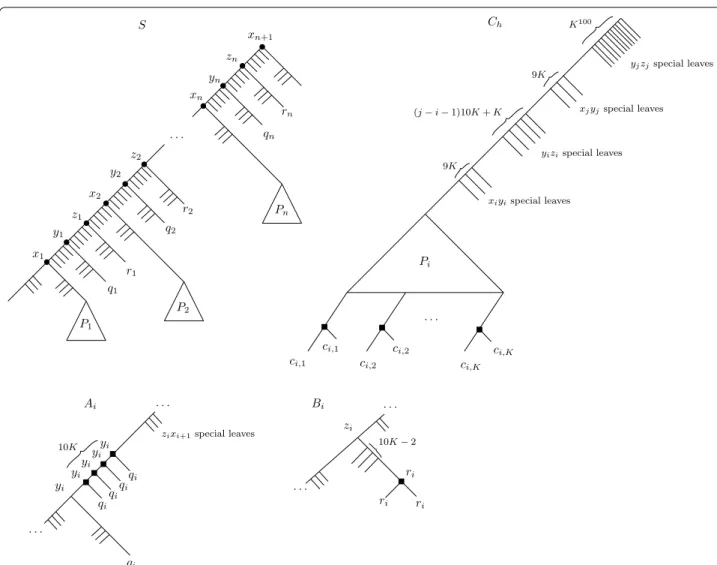
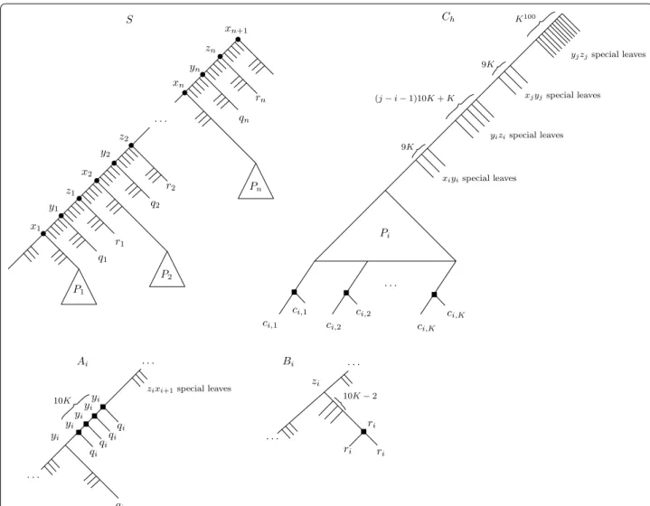
β <n ≪ K . We construct a species tree S and a gene forest G from G. The construction is relatively technical, but we will provide the main intuitions after having fully described it. For convenience, we will describe G as a set of gene trees instead of a single graph. Figure 3 illustrates the constructed species tree and gene trees. The con-struction of S is as follows: start with S being a caterpillar on 3n + 2 leaves. Let
be the path of this caterpillar consisting of the internal nodes, ordered by decreasing depth (i.e. x1 is the
deep-est internal node, and xn+1 is the root). For each i ∈ [n] ,
call pi, qi and ri , respectively, the leaf child of xi, yi and zi .
Note that x1 has two leaf children: choose one to name
p1 arbitrarily among the two. Then for each edge uv of S,
graft a large (but polynomial) number, say K100 , of leaves
on the uv edge (grafting t leaves on an edge uv consists of subdividing uv t times, thereby creating t new inter-nal nodes of degree 2, then adding a leaf child to each of these nodes, see Fig. 3). We will refer to these grafted leaves as the special uv leaves, and the parents of these leaves as the special uv nodes. These special nodes are the fundamental tool that lets us control the range of dupli-cation mappings.
Finally, for each i ∈ {1, . . . , n} , replace the leaf pi by a
tree Pi that contains K distinguished leaves ci,1, . . . , ci,K
such that dist(ci,j, r(Pi)) =K for all j ∈ [K] , and such
that dist(ci,j, lca(ci,j, ci,k)) ≥K /2 for all distinct j, k ∈ [K] .
By Lemma 5, each Pi can be constructed in polynomial
time. Note that the edges inside a Pi subtree do not have
special leaves grafted onto them. This concludes the con-struction of S.
We proceed with the construction of the set of gene trees G . Most of the trees of G consist of a subset of the nodes of S, to which we graft additional leaves to introduce duplications—some terminology is needed before proceeding. For w ∈ V (S) , deleting w consists in
removing w and all its descendants from S, then con-tracting the possible resulting degree two vertex (which was the parent of w if p(w) �= r(S) ). If this leaves a root with only one child, we contract the root with its child. For X ⊆ L(S) , keeping X consists of successively delet-ing every node that has no descendant in X until none remains (the tree obtained by keeping X is sometimes called the restriction of S to X).
The forest G is the union of three sets of trees A, B, C, so that G = A ∪ B ∪ C . Roughly speaking A is a set of trees corresponding to the choice of vertices in a vertex cover,
B is a set of trees to ensure that we “pay” a cost of one
for each vertex in the cover, and C is a set of trees cor-responding to edges. For simplicity, we shall describe the trees of G as having leaves labeled by elements of L(S) —a leaf labeled s ∈ L(S) in a gene tree T ∈ G is understood to be a unique gene that belongs to species s.
• The A trees Let A = {A1, . . . , An} , one tree for each
vertex of G. For each i ∈ [n] , obtain Ai by first taking
a copy of S, then deleting all the special yizi leaves.
Then on the resulting ziyi branch, graft 10K leaves
labeled qi . Then delete the child of zi that is also an
ancestor of ri (removing zi in the process). Figure 3
bottom-left might be helpful.
As a result, under the LCA-mapping µ , Ai has a path
of 10K duplications mapped to yi . One can choose
whether to keep this mapping in Ai , or to remap
these duplications to zi.
• The B trees Let B = {B1, . . . , Bn} . For i ∈ [n] , Bi is
obtained from S by deleting all except 10K − 2 of the special rizi leaves, and grafting a leaf labeled ri on the
edge between ri and its parent, thereby creating a
sin-gle duplication mapped to ri under µ.
Fig. 3 The species tree S, and the Ai,Bi and Ch trees. The internal nodes are labeled by their LCA-mapping µ , and black squares on the gene trees
• The C trees Let C = {C1, C2, . . . , Cm} , where for
h ∈ [m] , Ch corresponds to edge eh . Let vi, vj be the
two endpoints of edge eh= {vi, vj} , where i < j . To
describe Ch , we list the set of leaves that we keep
from S. Keep all the leaves of the Pi subtree of S, and
keep a subset of the special leaves defined as follows: – Keep 9K of the special xiyi leaves;
– Keep (j − i − 1)10K + K of the special yizi leaves;
– Keep 9K of the special xjyj leaves;
– Keep all the special yjzj leaves.
No other leaves are kept. Next, in the tree obtained by keeping the aforementioned list of leaves, for each k ∈ [K] we graft, on the edge between ci,k and
its parent, another leaf labeled ci,k . Thus Ch has K
duplications, all located at the bottom of the Pi
sub-tree. This concludes our construction.
Let us pause for a moment and provide a bit of intuition for this construction. We will show that G has a vertex cover of size β if and only if there exists a mapping α of G of cost at most 10Kn + β . As we will show later on, two Ai trees cannot have a duplication mapped to the same
species of S, so these trees alone account for 10Kn dupli-cations. The ri duplications in the Bi trees account for n
more duplications, so that if we kept the LCA-mapping, we would have 10Kn + n > 10Kn + β duplications. But some of these ri duplications could be remapped to zi , at
the cost of creating a path of 10K duplications to zi . This
is fine if Ai also has a path of 10K duplications to zi , as
this does not incur additional height. In this case, the Ai, Bi pairs introduces 10K duplications. If instead this
path in Ai is mapped to yi , we will show that remapping
ri is forbidden, summing up to 10K + 1 duplications for
such a particular Ai, Bi pair. The disadvantage of
remap-ping every to zi will become apparent when we consider
the Ch trees. The idea is that mapping the duplications of
Ai to yi represents including vertex vi in the vertex cover,
and mapping them to zi represents not including vi .
Because each time we map the Ai duplications to yi , we
have the additional ri duplication in Bi , we cannot do that
more than β times.
Now consider a Ch tree, eh= {vi, vj} . Under the
LCA-mapping, the ci,k duplications at the bottom enforce an
additional K duplications. This can be avoided by, say, mapping all these duplications to the same species. For instance, we could remap all these duplications to some yk species of S. But in this case, because of Lemma 3,
every node v of Ch above a ci,k duplication for which
µ(v) ≤ yk will become a duplication. This will create a
duplication subtree D in Ch with a large height, and our
goal will be to “reuse” the duplications we chose in the Ak′
and Bk′ trees. As it turns out, this “reuse” of duplications
will be feasible only if some yi or yj has duplication height
10K. If this does not occur, any attempt at mapping the ci,k nodes to a common species will induce a chain
reac-tion of too many duplicareac-tions created above.
The complete proof is somewhat technical. The inter-ested reader can find it in Appendix.
Theorem 2 The mprst-sd problem is NP-hard for
= 0 and for given δ > .
The above hardness supposes that δ and can be arbi-trarily far apart. This leaves open the question of whether MPRST-SD is NP-hard when δ and are fixed con-stants—in particular when δ = 1 + ǫ and = 1 , where ǫ <1 is some very small constant. We end this section by showing that the above hardness result persists event if only one gene tree is given. The idea is to reduce from the MPRST-SD shown hard just above. Given a species tree
S and a gene forest G , we make G a single tree by
incor-porating a large number of speciations (under µ ) above the root of each tree of G (modifying S accordingly), then successively joining the roots of two trees of G under a common parent until G has only one tree.
Theorem 3 The mprst-sd problem is NP-hard for
= 0 and for given δ > , even if only one gene tree is
given as input.
Proof We reduce from the mprst-sd problem in which
multiple trees are given. We assume that δ = 1 and = 0 and only consider duplications—we use the same argu-ment as before to justify that the problem is NP-hard for very small . Let S be the given species tree and G be the given gene forest. As we are working with the decision version of mprst-sd, assume we are given an integer t and asked whether costSD(G, S, α) ≤ t for some α . Denote
n = |L(G)| and let G1, . . . , Gk be the k > 1 trees of G .
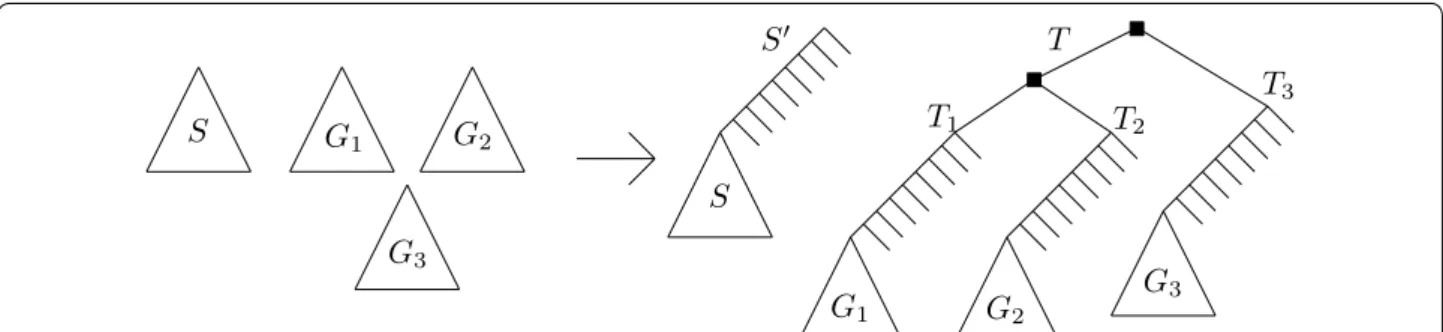
We construct a corresponding instance of a species tree S′ and a single gene tree T as follows (the construction
is illustrated in Fig. 4). Let S′ be a species tree obtained
by adding 2(t + k) nodes “above” the root of S. More precisely, first let C be a caterpillar with 2(t + k) internal nodes. Let l be a deepest leaf of C. Obtain S′ by replacing
l by the root of S. Then, obtain the gene tree T by
tak-ing k copies C1, . . . , Ck of C, and for each leaf l′ of each Ci
other than l, put s(l′) as the corresponding leaf in S′ . Then
for each i ∈ [k] , replace the l leaf of Ci by the tree Gi (we
keep the leaf mapping s of Gi ), resulting in a tree we call
Ti . Finally, let T′ be a caterpillar with k leaves h1, . . . , hk ,
and replace each hi by the Ti tree. The resulting tree is T.
We show that cost(G, S, α) ≤ t for some α if and only if cost(T, S′, α′) ≤t + k −1 for some α′.
Notice the following: in any mapping α of T, the k − 1 internal nodes of the T′ caterpillar must be duplications
mapped to r(S′) , so that h
α(r(S′)) ≥k −1 . Also note that
under the LCA mapping µ for T and S′ , the only
duplica-tions other than those k − 1 mentioned above occur in the Gi subtrees. The (⇒) is then easy to see: given α such that
cost(G, S, α) ≤ t , we set α′(v) = α(v) for every node v of T that is also in G (namely the nodes of G1, . . . , Gk ), and set
α′(v) = µ(v) for every other node. This achieves a cost of t + k −1.
As for the (⇐) direction, suppose that costSD(T′, S′, α′) ≤t + k −1 for some mapping α′ . Observe that under the LCA-mapping in T, each root of each Gi subtree has a path of 2(t + k) speciations in its
ances-tors. If any node in a Gi subtree of T is mapped to r(S′) , then
all these speciations become duplications (by Lemma 3), which would contradict costSD(T′
, S′, α′) ≤t + k −1 . We may thus assume that no node belonging to a Gi subtree is
mapped to r(S′) . Since h
α′(r(S′)) ≥k −1 , this implies that
the restriction of α′ to the G
i subtrees has cost at most t.
More formally, consider the mapping α′′ from G to S′
in which we put α′′
(v) = α′(v) for all v ∈ V (G) . Then costSD(G, S′, α′′) ≤costSD(T, S′, α′) − (k −1) ≤ t , because α′′ does not contain the top k − 1 duplications of
α′ , and cannot introduce longer duplication paths than in α′. We are not done, however, since α′′ is a mapping from G to
S′ , and not from G to S. Consider the set Q ⊆ V (G) of nodes
v of G such that α′′
(v) ∈ V (S) := V (S′) \V (S) . We will remap every such node to r(S) and show that this cannot increase the cost. Observe that if v ∈ Q , then every ancestor of v in G is also in Q. Also, every node in Q is a duplication (by invoking Lemma 2).
Consider the mapping α∗ from G to S′ in which we put
α∗(v) = α′′(v) for all v /∈ Q , and α∗(v) = r(S) for all v ∈ Q . It is not difficult to see that α∗ is valid.
Now, hα∗(s) =0 for all s ∈ V (S) and hα∗(s) = hα′′(s) for
all s ∈ V (S) \ {r(S)} . Moreover, the height of the r(S) dupli-cations under α∗ cannot be more than the height of the
for-est induced by Q and the duplications mapped to r(S) under α′′ . In other words,
Therefore, the sum of duplication heights cannot have increased. Finally, because α∗ is a mapping from G to S,
we deduce that costSD(G, S, α∗) ≤costSD(G, S′, α′′) ≤t ,
as desired.
An FPT algorithm
In this section, we show that for costs δ > and a parameter d > 0 , if there is an optimal reconciliation α of cost costSD(G, S) satisfying ˆd(α) ≤ d , then α can be
found in time O(⌈δ ⌉d·n ·
δ ).
In what follows, we allow mappings to be partially defined, and we use the ⊥ symbol to indicate undeter-mined mappings. The idea is to start from a mapping in which every internal node is undetermined, and gradu-ally determine those in a bottom-up fashion. We need an additional set of definitions. We will assume that δ > >0 (although the algorithm described in this sec-tion can solve the = 0 case by setting to a very small value).
We say that the mapping α : V (G) → V (S) ∪ {⊥} is a partial mapping if α(l) = s(l) for every leaf l ∈ L(G) , and it holds that whenever α(v) �= ⊥ , we have α(v′) �= ⊥ for every descendant v′ of v. That is, if a node
is determined, then all its descendants also are. This also implies that every ancestor of a ⊥-node is also a
hα∗(r(S)) ≤max Gi hα′′(r(S)) + � s′∈V (S) h(Gi[α′′, s′]) =hα′′(r(S)) +max Gi � s′∈V (S) h(Gi[α′′, s′]) ≤hα′′(r(S)) + � s′∈V (S) max Gi �h(Gi[α′′, s′]) � =hα′′(r(S)) + � s′∈V (S) h�G[α′′ , s′]� =hα′′(r(S)) + � s′∈V (S) hα′′(s′)
Fig. 4 The construction of S′ and T from S and the set of gene trees G
1, . . . ,Gk (here k = 3 ). The black squares indicate the path of k − 1 duplications
⊥-node. A node v ∈ V (G) is a minimal ⊥-node (under α ) if α(v) = ⊥ and α(v′) �= ⊥ for each child v′ of v. If α(v) �= ⊥ for every v ∈ V (G) , then α is called complete. Note that if α is partial and α(v) �= ⊥ , one can already determine whether v is an S or a D node, and hence we may say that v is a speciation or a duplication under α . Also note that the definitions of ˆd(α), l(α) and hα(s)
extend naturally to a partial mapping α by considering the forest induced by the nodes not mapped to ⊥.
If α is a partial mapping, we call α′ a
comple-tion of α if α′ is complete, and α(v) = α′(v) whenever
α(v) �= ⊥ . Note that such a completion always exists, as in particular one can map every ⊥-node to the root of S (such a mapping must be valid, since all ances-tors of a ⊥-node are also ⊥-nodes, which ensures that r(S) = α′(v) ≥ α′(v′) for every descendant v′ of a newly
mapped ⊥-node v). We say that α′ is an optimal
comple-tion of α if costSD(α′) is minimum among every possible
completion of α . For a minimal ⊥-node v with children v1 and v2 , we denote µα(v) = LCAS(α(v1), α(v2)) , i.e. the
lowest species of S to which v can possibly be mapped to in any completion of α . Observe that µα(v) ≥ µ(v) .
Moreover, if v is a minimal ⊥-node, then in any com-pletion α′ of α , α′[v → µ
α(v)] is a valid mapping. A
minimal ⊥-node v is called a lowest minimal ⊥-node if, for every minimal ⊥-node w distinct from v, either µα(v) ≤ µα(w) or µα(v) and µα(w) are incomparable.
The following Lemma forms the basis of our FPT algorithm, as it allows us to bound the possible map-pings of a minimal ⊥-node.
Lemma 6 Let α be a partial mapping and let v be a
minimal ⊥-node. Then for any optimal completion α∗ of
α , α∗(v) ≤ par⌈δ/ ⌉(µα(v)).
Proof Let α∗ be an optimal completion of α and let
α′:=α∗[v → µα(v)]. Note that ˆd(α′) ≤ ˆd(α∗) +1 .
Now suppose that α∗
(v) > par⌈δ/ ⌉(µα(v)) . Then by the
Shift-down lemma, l(α∗) −
l(α′) > ⌈δ/ ⌉ ≥ δ/ . Thus costSD(α∗) −costSD(α′) > −δ + (δ/ ) =0 . This contra-dicts the optimality of α∗ .
A node v ∈ V (G) is a required duplication (under α ) if, in any completion α′ of α , v is a duplication under α′ . We
first show that required duplications are easy to find.
Lemma 7 Let v be a minimal ⊥-node under α , and let
v1 and v2 be its two children. Then v is a required
duplica-tion under α if and only if α(v1) ≥ µ(v) or α(v2) ≥ µ(v).
Proof Suppose that α(v1) ≥ µ(v) , and let α′ be a
com-pletion of α . If α′
(v) = α′(v1) , then v is a duplication by
definition. Otherwise, α′
(v) > α′(v1) = α(v1) ≥ µ(v) ,
and v is a duplication by Lemma 2. The case when α(v2) ≥ µ(v) is identical.
Conversely, suppose that α(v1) < µ(v) and
α(v2) < µ(v) . Then α(v1) and α(v2) must be
incom-parable descendants of µ(v) (because other-wise if e.g. α(v1) ≤ α(v2), then we would have
µ(v) = LCAS(µ(v1), µ(v2)) ≤ LCAS(α(v1), α(v2)) = α(v2), whereas we are assuming that α(v2) < µ(v) ). Take
any completion α′ of α such that α′(v) = µ(v) . To
see that v is a speciation under α′ , it remains to
argue that α′(v) = µ(v) = LCA
S(α(v1), α(v2)) .
Since µ(v) is an ancestor of both α(v1) and α(v2) ,
we have LCAS(α(v1), α(v2)) ≤ µ(v). We also have
µ(v) = LCAS(µ(v1), µ(v2)) ≤LCAS(α(v1), α(v2)) , and
equality follows.
Lemmas 8 and 9 allow us to find minimal ⊥-nodes of G that are the easiest to deal with, as their mapping in an optimal completion can be determined with certainty.
Lemma 8 Let v be a minimal ⊥-node under α . If v is not
a required duplication under α , then α∗
(v) = µα(v) for
any optimal completion α∗ of α.
Proof Let v1, v2 be the children of v, and let α∗ be an
optimal completion of α . Since v is not a required duplica-tion, by Lemma 7 we have α(v1) < µ(v) and α(v2) < µ(v)
and, as argued in the proof of Lemma 7, α(v1) and α(v2)
are incomparable. We thus have that µα(v) = µ(v) . Then
α∗[v → µ(v)] is a valid mapping, and v is a speciation under this mapping. Hence ˆd(α∗[v → µ(v)]) ≤ ˆd(α∗) .
Then by the Shift-down lemma, this new mapping has fewer losses, and thus attains a lower cost than α∗ .
Lemma 9 Let v be a minimal ⊥-node under α , and let
αv:=α[v → µα(v)] . If ˆd(α) = ˆd(αv) , then α∗(v) = µα(v)
for any optimal completion α∗ of α.
Proof Let α∗ be an optimal completion of α . Denote
s := µα(v) , and assume that α∗(v) > s (as otherwise, we
are done). Let α′=α∗[
v → s] . We have that l(α′) <l(α∗) by the Shift-down lemma. To prove the Lemma, we then show that ˆd(α′) ≤ ˆ
d(α∗) . Suppose otherwise that ˆ
d(α′) > ˆd(α∗) . As only v changed mapping to s to go from α∗ to α′ , this implies that h
α′(s) > hα∗(s) because of
v. Since under α∗ , no ancestor of v is mapped to s, it must
be that under α′ , v is the root of a subtree T of height
hα′(s) of duplications in s. Since T contains only
descend-ants of v, it must also be that hαv(s) = hα′(s) (here αv is
the mapping defined in the Lemma statement). As we are assuming that hα′(s) > hα∗(s) , we get hα
v(s) > hα∗(s) .
This is a contradiction, since hα∗(s) ≥ hα(s) = hα
v(s) (the
strategy will be to “clean-up” the easy nodes, meaning that we map them to µα(v) as prescribed above, and
then handle the remaining non-easy nodes by branch-ing over the possibilities. We say that a partial mappbranch-ing α is clean if every minimal ⊥-node v satisfies the two following conditions:
[C1] v is not easy;
[C2] for all duplication nodes w (under α with α(w) �= ⊥ ), either α(w) ≤ µα(v) or α(w) is incomparable with µα(v).
Roughly speaking, C2 says that all further duplica-tions that may “appear” in a completion of α will be mapped to nodes “above” the current duplications in α . The purpose of C2 is to allow us to create duplication nodes with mappings from the bottom of S to the top. Our goal will be to build our α mapping in a bottom-up fashion in G whilst maintaining this condition. The next lemma states that if α is clean and some lowest minimal ⊥-node v gets mapped to species s, then v brings with it every minimal ⊥-node that can be mapped to s.
Lemma 10 Suppose that α is a clean partial mapping,
and let α∗ be an optimal completion of α . Let v be a
low-est minimal ⊥ -node under α , and let s := α∗
(v) . Then for
every minimal ⊥ -node w such that µα(w) ≤ s , we have
α∗(w) = s.
Proof Denote α′:=α[v → s]. Suppose first that
s = µα(v) . Note that since α is clean, v is not easy,
which implies that hα′(s) = hα(s) +1 . Since v is a
low-est minimal ⊥-node, if w is a minimal ⊥-node such that µα(w) ≤ s , we must have µα(w) = s , as otherwise v
would not have the ‘lowest’ property. Moreover, because
v and w are both minimal ⊥-nodes under the partial
map-ping α , one cannot be the ancestor of the other and so
v and w are incomparable. This implies that mapping w
to s under α′ cannot further increase h
α′(s) (because we
already increased it by 1 when mapping v to s). Thus ˆ
d(α′) = ˆd(α′[w → s]) , and w is easy under α′ and must be
mapped to s by Lemma 9. This proves the α∗(v) = µ α(s)
case.
and must be mapped to s <s , a contradiction. Thus assume s′> µ
α(v) . Under α∗ , for each child v′ of v, we
have α∗(v′) ≤ µ
α(v) < s′ , and for each ancestor v′′ of v,
we have α∗(v′′) ≥ α∗(v) = s > s′ . Therefore, by
remap-ping v to s′ , v is the only duplication mapped to s′ among
its ancestors and descendants. In other words, because hα∗(s′) >0 , we have ˆd(α∗[v → s′]) ≤ ˆd(α∗) . Moreover by
the Shift-down lemma, l(α∗[v → s′]) <l(α∗) , which
con-tradicts the optimality of α∗.
The remaining case is s′>s . Note that h
α∗(s) >0
(because v must be a duplication node, due to α being clean). Since it holds that v is a minimal ⊥-node, that α is clean and that s > µα(v) , it must be the case that α has
no duplication mapped to s (by the second property of cleanness). In particular, w has no descendant that is a duplication mapped to s under α (and hence under α∗ ).
Moreover, as s′=α∗(w) > s , w has no ancestor that is a
duplication mapped to s. Thus ˆd(α∗[w → s]) ≤ ˆd(α∗) ,
and the Shift-down lemma contradicts the optimality of
α∗ . This concludes the proof.
We are finally ready to describe our algorithm. We start from a partial mapping α with α(v) = ⊥ for every internal node v of G . We gradually “fill-up” the ⊥-nodes of α in a bottom-up fashion, maintaining a clean mapping at each step and ensuring that each decision leads to an optimal completion α∗ . To do this, we pick a lowest minimal ⊥
-node v, and “guess” α∗(v) among the ⌈δ/ ⌉ possibilities.
This increases some hα(s) by 1. For each such guess s, we
use Lemma 10 to map the appropriate minimal ⊥-nodes to s, then take care of the easy nodes to obtain another clean mapping. We repeat until we have either found a complete mapping or we have a duplication height higher than d. An illustration of a pass through the algorithm is shown in Fig. 5.
Notice that the algorithm assumes that it receives a clean partial mapping α . In particular, the initial map-ping α that we pass to the first call should satisfy the two properties of cleanness. To achieve this, we start with a partial mapping α in which every internal node is a ⊥-node. Then, while there is a minimal ⊥-node v that is not a required duplication, we set α(v) = µα(v) , which makes
v a speciation. It is straightforward to see that the
more minimal ⊥-nodes become speciations, and we can-not create any duplication node without increasing costSD
because α has no duplication. C2 is met because there are no duplications at all.
an optimal completion α∗ of α having ˆd(α∗) ≤d , or ∞ if
no such completion exists—assuming that the algorithm receives a clean mapping α as input. Thus in order to use induction, we must also show that at each recursive call
Fig. 5 An illustration of one pass through the algorithm. The species tree S is left and G has two trees (middle) and partial mapping α (labels are the lowercase of the species). Here α is in a clean state, and the algorithm will pick a lowest minimal ⊥-node (white circle) and try to map it to, say, H. The forest on the right is the state of α after applying this and cleaning up
2 There is a subtlety to consider here. What we have shown is that if there
exists a mapping α of minimum cost costSD
(G, S) with d(α) ≤ dˆ , then the
algorithm finds it. It might be that a reconciliation α satisfying d(α) ≤ dˆ
exists, but that the algorithm returns no solution. This can happen in the case that α is not of cost costSD(G, S).
The complexity follows from the fact that the algorithm creates a search tree of degree ⌈δ/ ⌉ of depth at most d. The main technicality is to show that the algorithm main-tains a clean mapping before each recursive call.2
Theorem 4 Algorithm 1 is correct and finds a
mini-mum cost mapping α∗ satisfying ˆd(α∗) ≤d , if any, in time
O(⌈δ ⌉d·n · δ ).
Proof We show by induction over the depth of the
search tree that, in any recursive call made to Algorithm 1 with partial mapping α , the algorithm returns the cost of
done on line 15, α′ is a clean mapping. We additionally
claim that the search tree created by the algorithm has depth at most d. To show this, we will also prove that every α′ sent to a recursive call satisfies ˆd(α′) = ˆd(α) +1.
The base cases of lines 3–5 are trivial. For the induc-tion step, let v be the lowest minimal ⊥-node chosen on line 7. By Lemma 6, if α∗ is an optimal completion of α
and s = α∗(v) , then µ
α(v) ≤ s ≤ par⌈δ/ ⌉(µα(v)) . We try
all the ⌈δ/ ⌉ possibilities in the loop on line 9. The for-loop on line 11 is justified by Lemma 10, and the for-loop on line 13 is justified by Lemmas 8 and 9. Assuming that α′ is clean on line 15, by induction the recursive call will return the cost of an optimal completion α∗ of α′ having
ˆ
d(α∗) ≤d , if any such completion exists. It remains to
argue that for every α′ sent to a recursive call on line 15,
our assumption, we then have α(z) > µα′(w) ≥ µα(w0) .
Then z cannot be a duplication under α , as otherwise α itself could not be clean (by C2 applied on z and w0 ). Thus
z is a newly introduced duplication in α′ , and so z was a ⊥
-node under α . Note that Algorithm 1 maps ⊥-nodes of G one after another, in some order (z1, z2, . . . , zk) . Suppose
without loss of generality that z is the first duplication node in this ordering that gets mapped to α′
(z) . There are two cases: either α′
(z) �= s , or α′(z) = s. Suppose first that α′
(z) �= s . Lines 10 and 11 can only map ⊥-nodes to s, and line 13 either maps speciation nodes, or easy nodes that become duplications. Thus when α′
(z) �= s , we may assume that z falls into the latter case, i.e. z is easy before being mapped, so that mapping
z to α′
(z) does not increase hα′(α′(z)) . Because z is the
first ⊥-node that gets mapped to α′
(z) , this is only pos-sible if there was already a duplication z0 mapped to α′(z)
in α . This implies that α(z0) = α′(z) > µα(w0) , and that
α was not clean (by C2 applied on z0 and w0 ). This is a
contradiction.
We may thus assume that α′
(z) = s . This implies µα′(w) < α′(z) = s . If w was a minimal ⊥-node in α , it
would have been mapped to s on line 11, and so in this case w cannot also be a minimal ⊥-node in α′ , as we
sup-posed. If instead w was not a minimal ⊥-node in α , then
w has a descendant w0 that was a minimal ⊥-node under
α . We have µα(w0) ≤ µα′(w) < s , which implies that
w0 gets mapped to s on line 11. This makes µα′(w) < s
impossible, and we have reached a contradiction. We deduce that z cannot exist, and that α′ is clean.
It remains to show that ˆd(α′) = ˆ
d(α) +1 . Again, let s be the chosen species on line 9. Suppose first that s = µα(v) .
Then hα[v→s](s) = hα(s) +1 , as otherwise v would be
easy under α , contradicting its cleanness. In this situa-tion, as argued in the proof of Lemma 10, each node w that gets mapped to s on line 11 or on line 13 is easy, and thus cannot further increase the height of the duplica-tions in s. If s > µα(v) , then hα[v→s](s) =1 = hα(s) +1 ,
since by cleanness no duplication under α maps to s. Here, each node w that gets mapped on line 11 has no descendant nor ancestor mapped to s, and thus the height does not increase. Noting that remapping easy nodes on line 13 cannot alter the duplication heights, we get in
both cases that ˆd(α[v → s]) = ˆd(α) + 1 . This proves the correctness of the algorithm.
As for the complexity, the algorithm creates a search tree of degree ⌈δ/ ⌉ and of depth at most d. Each pass can easily seen to be feasible in time O(δ/ · n) (with appro-priate pre-parsing to compute µα(v) in constant time,
and to decide if a node is easy or not in constant time as well), and so the total complexity is O(⌈δ/ ⌉dn · δ
) .
Experiments
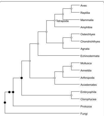
We used our software to reanalyze a data set of 53 gene trees for 16 eukaryotes presented in [14] and already reanalyzed in [1, 25]. In [1], the authors showed that, if segmental duplications are not accounted for, we get a solution having ˆd equal to 9, while their software (Exact-MGD) returns a solution with ˆd equal to 5. We were able to retrieve the solution with maximum height of 5 fix-ing δ ∈ [28, 61] and = 1 , but, as soon as δ > 61 , we got a solution with maximum height of 4 where no duplica-tions are placed in the branch leading to the Tetrapoda clade. The result is shown in Fig. 6 (also see [25, Fig. 1]). In [14], the Tetrapoda duplication was only supported by 6 trees (11.3%), whereas in our solution all these
Agnata Echinodermata Mollusca Anneldia Arthropoda Acoelemates Embryophita Clorophycea Protozoa Fungi
Fig. 6 The species tree phylogeny for the 16 eukaryotes studied
by Guigó et al. Black nodes indicate the location of segmental duplications detected by our algorithm (the 2 black circles suggest two consecutive segmental duplications)
duplications were remapped to the common ancestor of Chlorophyceae and Mammalia. The other locations of segmental duplications inferred in [14] are confirmed.3 This may sow some doubt on the actual existence of a segmental duplication in the LCA of the Tetrapoda clade.
We also reanalyzed the data set of yeast species described in [2]. First, we selected from the data set the 2379 gene trees containing all 16 species and refined unsupported branches using the method described in [16] and implemented in ecceTERA [15] with a bootstrap threshold of 0.9 and δ = = 1 . Using our method with δ =1.5 , = 1 we were able to detect the ancient genome duplication in Saccharomyces cerevisiae already estab-lished using synteny information [17], with 216 gene fam-ilies supporting the event. Other nodes with a signature of segmental duplication are nodes 7, 6, 13 and 2 (refer to Fig. 7) with respectively 190, 157, 148 and 136 gene fami-lies supporting the event. It would be interesting to see if the synteny information supports these hypotheses.
Note on the costs: As for any other parsimony method,
the costs associated to the events in Algorithm 1 (i.e. δ and ) have to be fixed by the user and cannot be esti-mated. Several possibilities exist to estimate these costs. A method for cost estimation for DL reconciliation, based on reducing large fluctuations in ancient genome
sizes, has been proposed in [6]. Another possibility is to use costs estimated by a maximum likelihood method, as done in [23], where the costs estimated in [27, 28] were used. Uncertainty in the input costs can also be tackled by considering several cost vectors and pareto-optimal reconciliations, or even via sampling; examples of these approach can be found respectively in [29] in the context of DTL reconciliations (i.e. DL reconciliations where hor-izontal gene transfers are also allowed) and in [4], where Boltzmann sampling is used in the context of evolution of gene adjacencies, a problem related to reconciliations. Conclusion
We have presented an approach for the reconciliation of a set of gene trees and a species tree, based on segmental macro-evolutionary events, where segmental duplication events and losses are associated with cost δ and , respec-tively. We have shown that the problem is polynomial-time solvable when δ ≤ , since LCA-mapping is already an optimal solution. When δ > the problem is NP-hard, even when = 0 and a single gene tree is given. This result solves a long standing open problem on the com-plexity of the reconciliation of a set of gene trees with a species tree. Moreover, we have given a fixed-parameter algorithm of time complexity O ⌈δ
⌉d·n · δ
, where d is the number of segmental duplications, that has been tested on real data, showing its effectiveness.
This work poses a variety of questions that deserve fur-ther investigation. The complexity of the problem when δ/ is a constant remains an open problem. Moreover, our FPT algorithm can handle data sets with a sum of duplication height of about d = 30 , but in the future, one might consider whether there exist fast approxima-tion algorithms for MPRST-SD in order to attain better scalability. Other future directions include a multivariate complexity analysis of the problem, in order to under-stand whether it is possible to identify other parameters that are small in practice. Finally, we plan to extend the experimental analysis to other data sets, for instance for the detection of whole genome duplications in plants. Authors’ contributions
RD, ML and CS all participated in writing the manuscript and establishing the theoretical results. ML implemented the algorithm, CS ran the experiments. All authors read and approved the final manuscript.
Author details
1 Dipartimento di Filosofia, Lettere, Comunicazione, Università degli Studi di Bergamo, Bergamo, Italy. 2 Department of Computer Science, Universitè de Sherbrooke, Sherbrooke, Canada. 3 ISEM, CNRS, IRD, EPHE, Universit de Mont-pellier, MontMont-pellier, France.
Acknowledgements
The authors would like to thank Mukul Bansal for providing the eukaryotes data set for the experiments section.
Fig. 7 The species tree phylogeny for the yeast data set described in
[2]. Numbers at the internal nodes are meaningless and are only used to refer to the nodes in the main text
3 Note that for this data set we used a high value for δ
since, because of the
sampling strategy, we expect that all relevant genes have been sampled (recall that in ExactMGD, is implicitly set to 0).
Not applicable.
Funding
The work of ML was supported by a postdoctoral fellowship from the Natural Sciences and Engineering Research Council (NSERC), Canada.
Appendix: Proof of Theorem 2 See Figs. 8 and 9.
there is a unique node w ∈ V (T) such that µ(w) = s . We then denote w by T[t]. In particular, any special node that is present in a tree T ∈ G satisfies the property, so when we mention the special uv nodes of T, we refer to the special nodes that are mapped to the corresponding spe-cial uv nodes in S under µ . For example in the Ch tree of
Fig. 3, the indicated set of (j − i − 1)10K + K nodes are
Fig. 8 The species tree S, and the Ai,Bi and Ch trees. The internal nodes are labeled by their LCA-mapping µ , and black squares on the gene trees
called special yizi nodes as they are mapped to the special
yizi nodes of S under µ.
We now show that G has a vertex cover of size β if and only if G and S admit a mapping α of cost at most 10Kn + β.
(⇒ ) Suppose that V′= {v
a1, . . . , vaβ} is a vertex cover
of G. We describe a mapping α such that for each i ∈ [n]: • If vi ∈V′ , then hα(yi) =10K , hα(ri) =1 and
hα(zi) =0;
• If vi∈/V′ , then hα(zi) =10K , hα(ri) =0 and
hα(yi) =0
and hα(w) =0 for every other node w ∈ V (S).
Summing over all i ∈ [n] , a straightforward verification show that this mapping α attains a cost of
It remains to argue that each tree can be reconciled using these duplications heights. In the remainder, we shall view these duplication heights as “free to use”, meaning that we are allowed to create a duplication path of nodes mapped to s ∈ V (S) , as long as this path has at most hα(s)
nodes, using hα defined above.
Let Ai∈A be one of the A trees, i ∈ [n] . If vi∈V′ is in
the vertex cover, then we have put hα(yi) =10K . In this
case, setting α(w) = µ(w) for every node w in Ai is a valid
s∈V (S) hα(s) = vi∈V′ (10K + 1) + vi∈V/ ′ 10K = 10Kn + β
mapping in which hα(s) described above is respected
for all s ∈ V (S) (the only duplications in Ai are those
10K mapped to yi ). If instead vi∈/V′ , then we may set
α(w) = zi for all the 10K original yi-duplications of Ai ,
and set α(w) = µ(w) for every other node. This is eas-ily seen to be valid since the ancestors of the original yi-duplications in Ai are all proper ancestors of zi.
Let Bi∈B be a Bi tree, i ∈ [n] . If vi ∈V′ , then
hα(ri) =1 , and so setting α(w) = µ(w) for all w ∈ V (Bi)
is valid and respects hα(s) for all s ∈ V (S) (since the ri
duplication is mapped to ri and there are no other
dupli-cations). If vi ∈/V′ , then set α(w) = zi for every node
between the original ri-duplication in Bi and Bi[zi] and set
α(w) = µ(w) for every other node w. This creates a path of 10K duplications mapped to zi , which is acceptable
since hα(zi) =10K . This case is illustrated in Fig. 9.
Let Ch∈W be a C tree, h ∈ [m] . Let vi, vj be the two
endpoints of edge eh= {vi, vj} , with i < j . Since V′ is a
vertex cover, we know that one of vi or vj is in V′ . Suppose
first that vi∈V′ . In this case, we have set hα(yi) =10K .
Let w be the highest special xiyi node of Ch (i.e. the
clos-est to the root). We set α(w) = yi for each internal node
descending from w. All of these nodes become duplica-tions, but the number of nodes of a longest path from w to an internal node descending from w is 10K (K for the Ri subtree, plus 9K for the special xiyi nodes). Thus
hav-ing hα(yi) is sufficient to cover the whole subtree rooted
![Fig. 7 The species tree phylogeny for the yeast data set described in [2]. Numbers at the internal nodes are meaningless and are only used to refer to the nodes in the main text](https://thumb-eu.123doks.com/thumbv2/123doknet/13721434.435448/15.892.85.436.131.488/species-phylogeny-yeast-described-numbers-internal-nodes-meaningless.webp)