HAL Id: ird-00270954
https://hal.ird.fr/ird-00270954
Submitted on 8 Apr 2008
HAL is a multi-disciplinary open access archive for the deposit and dissemination of sci-entific research documents, whether they are pub-lished or not. The documents may come from teaching and research institutions in France or abroad, or from public or private research centers.
L’archive ouverte pluridisciplinaire HAL, est destinée au dépôt et à la diffusion de documents scientifiques de niveau recherche, publiés ou non, émanant des établissements d’enseignement et de recherche français ou étrangers, des laboratoires publics ou privés.
To cite this version:
T. Condom, Anne Coudrain, Jean-Emmanuel Sicart, Sylvain Théry. Computation of the space and time evolution of equilibrium-line altitudes on Andean glaciers (10 degrees N-55 degrees S). Global and Planetary Change, Elsevier, 2007, 59 (1-4), pp.189-202. �10.1016/j.gloplacha.2006.11.021�. �ird-00270954�
websites are prohibited.
In most cases authors are permitted to post their version of the article (e.g. in Word or Tex form) to their personal website or institutional repository. Authors requiring further information
regarding Elsevier’s archiving and manuscript policies are encouraged to visit:
Computation of the space and time evolution of equilibrium-line
altitudes on Andean glaciers (10°N
–55°S)
Thomas Condom
a,⁎
, Anne Coudrain
b, Jean Emmanuel Sicart
b, Sylvain Théry
caInstitut EGID, University of Bordeaux 3, 1 allée Daguin,33607 Pessac Cedex, France b
IRD, Great Ice, BP 64501, 34394 Montpellier, France c
UMR Sisyphe, CNRS-UPMC, case 123, 4 place Jussieu, 75252 Paris Cedex 05, France Available online 9 January 2007
Abstract
A previous study of Fox [Fox, A.N. 1993. Snowline altitude and climate at present and during the Last Pleistocene Glacial Maximum in the Central Andes (5°–28°S). Ph.D. Thesis. Cornell University.] showed that for a fixed 0 °C isotherm altitude, the equilibrium-line altitude (ELA) of the Peruvian and Bolivian glaciers from 5 to 20°S can be expressed based on a log–normal expression of local mid-annual rainfall amount (P). In order to extrapolate the function to the whole Andes (10°N to 55°S) a local 0 °C isotherm altitude is introduced. Two applications of this generalised function are presented. One concerns the space evolution of mean inter-annual ELA for three decades (1961–1990) over the whole South American continent. A high-resolution data set (grid data: 10′ for latitude/longitude) of mean monthly air surface temperature and precipitation is used. Mean annual values over the 1961–1990 period were calculated. On each grid element, the mean annual 0 °C isotherm altitude is determined from an altitudinal temperature gradient and mean annual temperature (T ) at ground level. The 0 °C isotherm altitude is then associated with the annual precipitation amount to compute the ELA. Using computed ELA and the digital terrain elevation model GTOPO30, we determine the extent of the glacierised area in Andean regions under modern climatic conditions. The other application concerns the ELA time evolution on Zongo Glacier (Bolivia), where inter-annual ELA variations are computed from 1995 to 1999. For both applications, the computed values of ELA are in good agreement with those derived from glacier mass balance measurements.
© 2006 Elsevier B.V. All rights reserved.
Keywords: Andean glaciers; equilibrium-line altitude (ELA); precipitation; temperature; mass balance
1. Introduction
Glacier advances and retreats are normally linked with climate variations. These variations generate changes in rates of accumulation and ablation. Accu-mulation includes all processes that increase the glacier mass (predominantly snowfall, to a lesser extent vapor
condensation, snow and ice avalanches, wind contribu-tion). Ablation encompasses all processes that produce mass deficit, particularly sublimation and melting. At an annual time-scale, a glacier can be divided in an up-stream zone where accumulation processes dominate and a downstream zone where ablation processes dominate. The annual equilibrium-line altitude (ELA) delimits these two zones and is approximately equiva-lent to the annual snowline, that is, the lower boundary where snow cover remains at the end of the ablation season (Paterson, 1994). The mass balance is a sum of
Global and Planetary Change 59 (2007) 189–202
www.elsevier.com/locate/gloplacha
⁎ Corresponding author. Tel.: +33 557 12 10 15; fax: +33 557 12 10 01. E-mail address:condom@egid.u-bordeaux.fr(T. Condom).
0921-8181/$ - see front matter © 2006 Elsevier B.V. All rights reserved. doi:10.1016/j.gloplacha.2006.11.021
the ablation and accumulation terms. A stable ELA characterizes a long-term balance in equilibrium.
Several approaches can be used to study the ELA evolution over glaciers. The energy balance method
studies the energy fluxes to quantify the glacier ab-lation (Wagnon et al., 1998; Kull and Grosjean, 2000). It requires a large number of meteorological variables and complex field measurements. Other
Fig. 1. A Mean annual precipitation of Latin America for 1961–1990 (New et al., 2000). B Mean annual temperature of Latin America for 1961–1990 (New et al., 2000).
statistical and analytical methods are also used to link climate variables with the ELA and also with glacial retreats and advances. The glacial behaviour, and therefore the ELA, can be deduced in first approx-imation from climatic variables like temperature and
precipitation (Kuhn, 1989; Ohmura et al., 1992; Seltzer, 1994). In principle the ELA rises with tem-perature increase and/or a precipitation decrease and falls with a temperature decrease and/or precipitation increase.
}
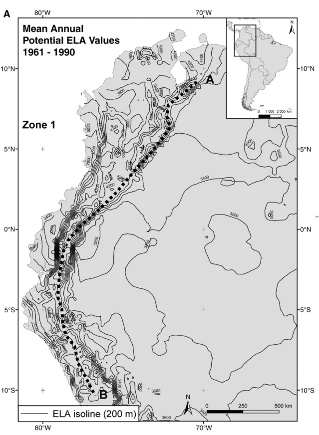
Fig. 2. A, B, C. Calculated potential equilibrium-line altitude (ELA) along three transects: A) Zone 1 with the A–B North/South transect from 10°N to 10°S; B) Zone 2 with B–C eastern and western transects from 10°S to 33°S; C) Zone 3 with the C–D North/South transect from 33°S to 55°S. Numbers represent different locations: 1 — Pico Humboldt (Venezuela); 2 — Ruiz–Tolima massif (Colombia), 3 — Equadorian volcanoes, 4 — Cordillera Blanca (Peru), 5 — Cordillera Real (Bolivia), 6 — Cordillera Occidental (Bolivia), 7 — Northern Patagonia Ice Field (Chile), 8 — Southern Patagonia Ice Field (Chile), 9 — Cordillera Darwin (Chile). The curved dashed segments represent the axis of the Andean Cordillera in Zones 1 and 2, and the border of the Cordillera in Zone 3.
Fox (1993) derived the ELA of 21 Peruvian and Bolivian glaciers as a function of the annual pre-cipitation. The objective of this paper is to generalize Fox's expression taking into account temperature variations in order to support estimation of the space
evolution of the ELA through the entire Andes, and to estimate the time evolution of the ELA for different years at a specific location. More precisely, this paper presents: (i) the mean values of the computed ELA and the modeled glacierised area map for the period 1961–
1990 in South America; and (ii) a comparison between ELA derived from mass balance data and ELA computed with the generalized expression for Zongo Glacier (16°15′S, 68°07′W, Bolivia), Glacier de Los Tres (49°16′S,73°00°W, Argentina) and Pío XI glacier (49° 3′S, 73°54′W, Chile).
2. Study area
The study area encompasses the Andean Cordillera region on the western part of the South American con-tinent where modern glaciers are located. The terminus and the ELA of Andean glaciers vary along North/South
and East/West transects. Schwerdtfeger (1976)divides the Andes' settings into three zones characterized by their climate conditions: 10°N to 12°S, 12° to 28°S, and 28° to 55°S.
From 10°N to 12°S the annual snowline is situated near 4700 m a.s.l. The glacier terminus ranges from 4100 to 5000 m a.s.l. and the 0 °C isotherm level shows little seasonal variations. In this high tropical zone the ELA is located close to the atmospheric 0° C isotherm level (Kuhn, 1981). This region is under easterly flux influence at mid-troposphere level throughout the year, and the temperature is a reliable indicator of glacial extension (Seltzer, 1990).
From 12° to 28°S, the annual snowline rises from 4700 m a.s.l. to 6000 m a.s.l. due to reduced preci-pitation associated with predominant anticyclonic con-ditions on the Pacific Ocean (Fig. 1A). At 25°S, given the strong inter-annual climatic variations, the 0 °C isotherm level could vary by 500 m from one year to another. The ELA is situated in this zone about 1000 m above the 0 °C isotherm level. The incoming moist Amazonian air causes an East/West gradient of the ELA ranging up to 500 m across the Central Andes, with a higher ELA in the Western part compared to the Eastern part. This region has a sub-tropical climate regime with alternate westerlies (during the austral winter) and easterlies (during the austral summer). The Zongo gla-cier (Bolivia) is located in this region at 16°15′S, 68°07′°W (seeFig. 1A).
From 28° to 55° S, the annual snowline falls from 6000 to 1000 m a.s.l. due to an increase in precipitation. In this area, glacier terminus fluctuates from 5900 m a.s. l. to sea level and the 0 °C isotherm lies between 500 and 4000 m a.s.l. Here westerlies dominate the annual wind regime bringing Pacific moist air towards the Andes, with a temperate climatic regime (Kuhn, 1981). The glaciers de Los Tres (Argentina) and Pío XI are located here at 49°16′S, 73°00°W and 49° 3′S, 73°54′W res-pectively (Fig. 1A).
Thus, the spatial distribution of glaciers between 10°N and 55°S is a function of various climatic regimes at local, regional and global scales.
3. Methods
We established an empirical relation based on the study of Fox (1993). For 21 Andean glaciers situated between 5° and 20°S,Fox (1993)established an empi-rical relation (Eq. (1)) between the annual normalized snowline altitude Y (m a.s.l.) and the annual precipita-tion amount P (mm yr− 1). The “normalized snowline altitude” is defined as the difference between the
re-gional snowline altitude and the altitude of the annual 0 °C isotherm for Peruvian (Eq. (2)) and Bolivian glaciers (Eq. (3)). This normalized snowline altitude is used to directly compare the effect of precipitation on the snow line altitude in the Peruvian and Bolivian Andes:
Y ¼ 3427−1148⁎log10ð ÞP ð1Þ
For Peruvian glaciers, the relation between the nor-malized snowline Y and annual ELA (m a.s.l.) can be defined byFox (1993)as:
Y ¼ ELA−4920 ð2Þ
where the mean annual 0 °C isotherm altitude is 4920 m a.s.l. in Peru.
For Bolivian glaciers defined byFox (1993):
Y ¼ ELA−4800 ð3Þ
where the mean annual 0 °C isotherm altitude is 4800 m a.s.l. in Bolivia.
Eqs. (2) and (3) can be rewritten based on a Iso0 term which reflects the mean annual altitude of the 0 °C isotherm level (Eq. (4)):
Y ¼ ELA−Iso0 ð4Þ
Finally, replacing Eq. (4) into Eq. (1) the ELA can be formulated as:
ELA¼ 3427−1148 logð 10ð ÞP Þ þ Iso0 ð5Þ
The Iso0 term (Eq. (6)) can be derived from a vertical temperature gradient of 0.7 °C/ 100 m following Acei-tuno (1996), where T is the mean annual temperature at a station located at ground level (°C) and z is the station elevation in m a.s.l.:
Iso0¼ T=0:007 þ z ð6Þ
Therefore, the annual ELA can be calculated as: ELA¼ 3427−1148 logð 10ð ÞP Þ þ T=0:007 þ z ð7Þ where the ELA is in m a.s.l., and P is the annual precipitation amount (mm yr− 1). While the previous formulation (Eq. (1)) contained only one variable (P) the new formulation depends on two variables: annual tem-perature (T ) and precipitation amount (P) (Eq. (7)).
In extra-tropical regions the accumulation period takes place mostly during winter and almost all ablation occurs in summer, while in the tropical region a clear cut
separation between the accumulation and the ablation seasons is not observed (Kaser et al., 1996). In the tropics, most snow accumulation occurs during the summer wet season, while during the wintertime, precipitation amount is too weak to have a significant impact on the glacier mass balance (Francou et al., 1995; Ribstein et al., 1995), and ablation occurs all year round (Kaser et al., 1996).
Eq. (7) allows to calculate the ELA from precipi-tation, temperature and station elevation data available locally. This relation is easy to use for determining the approximate spatial and temporal evolution of the ELA. Using an inverse method, it also enables to elaborate paleoclimatic reconstructions by defining a range of possible temperatures and precipitation amounts com-patible with available paleo-ELA informations. How-ever, before applying this expression to modern, past or future conditions, it is necessary to verify the vali-dity of Eq. (7) on the base of instrumented data series for a recent period. This is the purpose of the following section.
4. Test of validity for a modern period
4.1. Calculations of Andean ELAs and glacierised area for the 1961–1990 period
The climatic and topographic data bases used for all of South America are those ofNew et al. (2000). Indeed, this modern climatic data base includes mean monthly
temperature (T ) and precipitation (P) for 1961–1990, at a spatial resolution of 10′ for the entire globe.
The first step is to calculate the mean inter-annual values of T and P that are presented inFig. 1A and B. Then, using Eq. (7), the mean inter-annual ELA values are calculated for this period.
The spatial variations of the computed ELAs are presented inFig. 2A, B and C for three latitude ranges. In these figures the iso-values of ELA reflect only potential ELAs (ELAp); for locations where the computed ELA is higher than the actual Earth's surface elevation (Es), it represents only a theoretical situation. Therefore, the discussion on the comparison of computed ELA and available data presented in the following paragraphs only concerns the high-elevation Andean regions where ELApbEs.
In the Northern zone (Zone 1, Fig. 2A), along the transect A–B, the computed ELA is relatively constant, ranging between 4200 and 5000 m a.s.l.. We find a good agreement between computed values and observations: (i) in Venezuela, the snowline is at 4700 m a.s.l. in the Sierra Nevada de Mérida (71°W, 8.54°N) (Schubert, 1992); (ii) in Colombia, the ELA ranges between 4800 and 4900 m a.s.l. in the Ruiz–Tolima massif in 1976 (75.33°W, 4.88°N) (Hoyos-Patiño, 2003); and (iii) on Ecuadorian Volcanoes (78°W–79°W, 0.5°N–2°S), the ELA is located between 4800 and 4900 m a.s.l. ( Has-tenrath, 1981).
In the mid-latitude zone (Zone 2, Fig. 2B), along the transect B–C, the computed ELA rises from 4600 to
Fig. 3. Mean annual potential calculated ELA along Andean transects from 15°N to 55°S and annual snowline given in the World Glacier Inventory by theNational Snow and Ice Data Center (1999).
6200 m a.s.l. southwards from 10°S to 25°S. Along the West–East transect E–F (Zone 2,Fig. 2B), the computed ELA increases from the oriental to the occidental cor-dillera. These changes in computed ELA along the two
transects (eastern and western) are directly related to the Amazonian moisture source. These results are in good agreement with those obtained byHastenrath and Morales-Arnao (2003)in Cordillera Blanca, Peru (77°W– 78°W,
Fig. 4. A, B, C. Calculated glacierised areas in the Andean region: A) Zone 1 from 10°N to 10°S; B) Zone 2 from 10°S to 33°S; C) Zone 3 from 33°S to 55°S. Numbers represent different locations: 1— Pico Humboldt (Venezuela); 2 — Ruiz–Tolima massif (Colombia), 3 — Equadorian Volcanoes, 4— Cordillera Blanca (Peru), 5 — Cordillera Real (Bolivia), 6 — Cordillera Occidental (Bolivia), 7 — Northern Patagonia Ice Field (Chile), 8— Southern Patagonia Ice Field (Chile), 9 — Cordillera Darwin (Chile).
8°S–10°S), where they observed an ELA ranging from 4850 to 4900 m a.s.l. in 1977–1981. South of 25°S, the calculated ELA drops from 6200 to 4600 m a.s.l. at 33°S. In the Southern zone (Zone 3, Fig. 2C), along the transect C–D, the computed ELA decreases from 4600 m a.s.l. at 33°S to 1000 m a.s.l. at 55°S in good
accordance with the southward increase of moist air from the Pacific Ocean.
ELA calculations were compared with field results on two extra-tropical glaciers. At Glacier de los Tres in Argentina (49°16′30″ S/73° 00′ 30″ W) the mean annual calculated potential ELA value was 1417 m a.s.l., while
based on observations from Popovnin et al. (1999) in 1995–1996 the ELA was 1440 m a.s.l. Similarly, the calculated ELA for Pío XI Glacier (49° 3′S, 73°54′W) was 1080 m a.s.l., very similar to the observed value of 1100 m a.s.l. given byRivera and Casassa (1999)during the summer of 1994–1995. Differences between
calcu-lated and measured ELA values of less than 40 m confirm the robustness of Eq. (7) for non-tropical glaciers.
To validate the calculated ELAs along the North/ South (A to C) transect, we used observed annual snow line elevations (m a.s.l.) provided by theNational Snow and Ice Data Center (1999) in the World Glacier
Inventory (WGI) database. These data, issued from the National Snow and Ice Data center (NSIDC), are provided from field work, air photos and high-resolution satellite imagery for the 1955–1999 period.
Fig. 3 demonstrates that the ELA variations, as described before, are in good agreement with the WGI database. However, some discrepancies appear near 30°S. This can be related to the large ELA East/West gradient that is likely to contribute to a large variability of the ELA especially close to 30°S where the transect presents the computed results only for one longitude at each latitude.
A combined approach allows the determination of glacierised extensions for the entire Andes region. This can be computed, as a first-order approach, by sub-tracting the Earth's surface elevation from the computed ELA. Locations where the difference is positive are considered as glacierised. This assumes that the low-ermost boundary of glacier areas corresponds to the ELA, which is not true, particularly for Patagonia and Tierra del Fuego where glacier fronts can reach ele-vations more than 1000 m below their ELAs (Rivera and
Casassa, 1999). Topographic data are extracted from the modified GTOPO30 (1996) digital elevation model (DEM). This DEM is defined by a horizontal grid spacing of 30″ (approximately 1 km) and elevations were shifted by −28 m to be in better agreement with 1:50 000 maps of central Andes region (Condom et al., 2004). Glaciers are presented onFig. 4A, B and C. As shown on these figures, major glacierised areas are in general well represented.
4.2. ELA inter-annual variations on Zongo Glacier (1994–1999)
The purpose here is to verify the ability of the proposed Eq. (7) to reproduce the inter-annual variations of the ELA. The ELA is computed for Zongo Glacier over the period 1995–1999, considering that the hy-drological year starts September 1. Meteorological data, precipitation and temperature were measured at a mete-orological station situated on a lateral moraine (5165 m a.s.l.) (Leblanc et al., 2000). Results are shown onFig. 5
and inTable 1. We compare computed ELA with mass balance measurements obtained from stakes and snow-pits. The ELA calculated from Eq. (7) ranges between 4943 and 5356 m a.s.l. while the field-based ELA ranges from 4993 to 5437 m a.s.l. (Sicart et al., 2007-this issue). However, due to the absence of stakes between 5200 and 5400 m a.s.l., uncertainties on the field-based ELAs are large. Considering one specific year the differences between both methods can be substantial (around 150 m) but the magnitudes and inter-annual variations are similar over the 1994–1999 period.
5. Discussion and conclusion
A glacier is in continuous evolution in response to the variations of climate forcings. We should consider that each glacier is a unique case, with varying exposure, slope, surface area, substrata, etc. Thus, a regional ap-proach can be inappropriate when it is applied at the local scale (Klein et al., 1999; Dornbush, 2001). Fur-thermore, the changes in size and the growth of glaciers
Table 1
Meteorological data and ELA on Zongo glacier for 1994–1999 Hydrological year P mm yr− 1 T at 5156 m a.s.l. °C Isotherm 0 °C level m a.s.l.
Calculated ELA with Eq. (7) m a.s.l.
Calculated ELA by mass balance method m a.s.l.
1994–1995 723 −0.25 5130 5275 5374
1995–1996 925 −0.85 5044 5066 5350
1996–1997 1050 −1.27 4984 4943 4993
1997–1998 780 0.59 5249 5356 5437
1998–1999 1033 −0.92 5034 5001 5170
Fig. 5. Inter-annual ELA variations on Zongo glacier for 1995–1999 (Sicart, 2002).
can result from complex interactions between climate, topography and ice dynamics. In our study, the spatial resolution is limited by a 30 arc second wide grid of the DEM. The advantage of our method lies on its simpli-city, i.e. the only requested variables are temperature, precipitation and elevation. This makes it easy to de-lineate space and time evolutions.
This study is based on the same principles asKuhn (1979) who demonstrated that on mid-latitude and tropical glaciers, the ELA changes can be derived from the isotherm 0 °C altitude and the precipitation amount. More precisely, glaciers in the inner humid tropical regions are more sensitive to air temperature variations than in the arid sub-tropical zones where the impacts of the humidity changes are stronger (Kaser, 2001). Our extrapolation to the entire Andes provides valuable information on the spatial variation of ELA over large spatial scales. Zongo Glacier (Bolivia), Glacier de Los Tres (Argentina) and Pío XI Glacier (Chile) case studies demonstrate the utility of the method to highlight the inter-annual variability of the ELA both in tropical and temperate regions.
The main advantage of our empirical approach is that Eq. (7) is easy to apply under different climatic settings. This method is valid for all of the Andes under modern conditions and can be used to explore precipitation/ temperature schemes at the origin of the glacier repar-titions during and since the Last Glacial Maximum. Furthermore, in a global warming context, it can be useful to estimate the glacial trends at the regional scale and perhaps even globally, even though other ap-proaches based on energy balance studies are crucial for calibration of the method.
Acknowledgements
The authors thank the following organizations for their help in data gathering and their financial support: the GREAT ICE program from I.R.D (Institut de Re-cherche pour le Développement), the French national programs PNRH (2002) and ECLIPSE (2002). We are grateful to Shannon Sterling for useful comments and suggestions. Furthermore, we wish to thank the two anonymous reviewers for their relevant comments and detailed suggestions.
References
Aceituno, P., 1996. Elementos del clima en el altiplano sudamericano. Rev. Geofís. 44, 37–55.
Condom, T., Coudrain, A., Dezetter, A., Brunstein, D., Delclaux, F., Sicart, J.E., 2004. Transient modelling of lacustrine regressions.
Two case studies from the Andean Altiplano. Hydrol. Proc. 18, 2395–2408.
Dornbush, U., 2001. Correspondence on:. Modern and last local glacial maximum snowlines in the Central Andes of Peru, Bolivia and Northern Chile. Quater. Sc. Rev. 18, 63–84. Quat. Sci. Rev. 20, 1153–1158.
Fox, A.N., 1993. Snowline altitude and climate at present and during the Last Pleistocene Glacial Maximum in the Central Andes (5°–28°S). Ph.D. Thesis. Cornell University.
Francou, B., Ribstein, P., Saravia, R., Tiriau, E., 1995. Monthly balance and water discharge of an inter-tropical glacier: Zongo glacier Cordillera Real, Bolivia, 16°S. J. Glaciol. 41 (n°137), 61–67.
GTOPO30, 1996. US Geological Survey EROS Data Center in Sioux Falls, South Dakota.http://edcdaac.usgs.gov/gtopo30/gtopo30.asp. Hastenrath, S., 1981. The Glaciation of the Ecuadorian Andes. A.A.
Balkema Publishers, Rotterdam.
Hastenrath, S., Morales-Arnao, B., 2003. Glaciers of Peru. Satellite Image Atlas of Glaciers of the World. USGS. Site:http://pubs.usgs. gov/.
Hoyos-Patiño, F., 2003. Glaciers of Colombia. Satellite Image Atlas of Glaciers of the World. USGS. Site:http://pubs.usgs.gov/. Kaser, G., 2001. Glacier–climate interaction at low-latitudes. J.
Gla-ciol. 47 (n°157), 195–204.
Kaser, G., Hastenrath, S., Ames, A., 1996. Mass balance profiles on tropical glaciers. Z. Gletsch.kd. Glazialgeol. 32, 75–81.
Klein, A.G., Seltzer, G.O., Isacks, B.L., 1999. Modern and last local glacial maximum snowlines in the Central Andes of Peru, Bolivia and Northern Chile. Quat. Sci. Rev. 18, 63–84.
Kuhn, M., 1979. Climate and Glaciers. Sea Level, Ice, and Climatic Change (Proceedings of the Canberra Symposium, December 1979). IAHS Publ., p. 131.
Kuhn, M., 1981. Vergletscherung, Nullgradgrenze, und Niederschlag in den Anden. Springer-Verlag, Wien.
Kuhn, M., 1989. The response of the equilibrium line altitude to climate fluctuations: theory and observations. In: Oerlemans, J. (Ed.), Glacier Fluctuations and Climate Change. Kluwer, Dordrecht, pp. 407–417.
Kull, C., Grosjean, M., 2000. Late Pleistocene climate conditions in the north Chilean Andes drawn from a climate–glacier model. J. Glaciol. 46 (n°155), 622–632.
Leblanc, J.M., Sicart, J.E., Gallaire, R., Chazarin, J.P., Ribstein, P., Pouyaud, B., Francou, B., Baldivieso, H., 2000. Mesures météo-rologiques, hydrologiques et glaciologiques, années hydrologiques 1997–98. IRD 1. Rapport.
National Snow and Ice Data Center, 1999. World Glacier Inventory. World Glacier Monitoring Service and National Snow and Ice Data Center/World Data Center for Glaciology. Digital Media, Boulder CO.
New, M., Lister, D., Hulme, M., Makin, I., 2000. A high-resolution data set of surface climate over global land areas. Clim. Res. 21, 1–25.
Ohmura, A., Kasser, P., Funk, M., 1992. Climate at the equilibrium line of glaciers. J. Glaciol. 38, 397–411.
Paterson, W.S.B., 1994. The Physics of Glaciers, Third Edition. Pergamon, New York.
Popovnin, V.V., Danilova, T.A., Petrakov, D.A., 1999. A pioneer mass balance estimate for a Patagonian glacier: Glaciar De los Tres, Argentina. Glob. Planet. Change 22, 255–267.
Ribstein, P., Tiriau, E., Francou, B., Saravia, R., 1995. Tropical climate and glacier hydrology; a case study in Bolivia. J. Hydrobiol. 165 (n°1–4), 221–234.
Rivera, A., Casassa, G., 1999. Volume changes on Pío XI glacier, Patagonia:1975–1995. Glob. Planet. Change 22, 233–244. Schubert, C., 1992. The glaciers of the Sierra Nevada de Mérida
(Venezuela), a photographic comparison of recent deglaciation. Erdkunde 46, 58–64.
Schwerdtfeger, W., 1976. Introduction in“Climates of Central and South America”. In: Schwerdtfeger, W. (Ed.), World Survey of Climatology. Elsevier Scientific, New York.
Seltzer, G.O., 1990. Recent glacial history and paleoclimate of the Peruvian–Bolivian Andes. Quat. Sci. Rev. 20, 137–152. Seltzer, G.O., 1994. Climatic interpretation of alpine snowline
varia-tions on millenial timescales. Quat. Res. 41, 154–159.
Sicart, J.M., 2002. Contribution à l'étude des flux d'énergie, du bilan de masse et du débit de fonte d'un glacier tropical: le Zongo, Bolivia. Ph.D. Thesis. Paris 6 University, France.
Sicart, J.E., Ribstein, P., Francou, B., Pouyaud, B., Condom, T., Yoshida, N., Matoba, S., Godoi, M.A., 2007. Hydrological and glaciological mass balances of a tropical glacier: Zongo, Bolivia. Glob. Planet. Change. 59, 27–36 (this issue). doi:10.1016/j. gloplacha.2006.11.024.
Wagnon, P., Ribstein, P., Schuler, T., Francou, B., 1998. Flow sepa-ration on Zongo Glacier, Cordillera Real, Bolivia. Hydrol. Proc. 12, 1911–1926.