Active control of buckling : centralized and decentralized approaches

(1)

Active Control of Buckling:

Centralized and Decentralized Approaches

by

Natalya Cohen

Submitted to the Department of Electrical Engineering and Computer Science in Partial Fulfillment of the Requirements for the Degrees of

Bachelor of Science in Electrical Engineering and Computer Science and Master of Engineering in Electrical Engineering and Computer Science

at the Massachusetts Institute of Technology May 23, 1996

The author hereby grants to M.I.T. permission to reproduce and distribute publicly paper and electronic copies of this thesis

and to grant others the right to do so.

MASSACHUS-TTS INST',TU"TE OF TECHNOLOGY

JUN

111996

LIBRARIES 1-C: tUbllU

Department of Electrical Engineerin and Computer Science

/I e- - May 23,1996

:ertified by

,

--

-Gerald J. Sussman Stsulhia Profess of Electrical Engineering

ý Thesis Supervisor

kccepted by

F. R. Morgenthaler tee on Graduate Theses _~~·

A ,,t,

(2)

Active Control of Buckling:

Centralized and Decentralized Approaches

by

Natalya Cohen

Submitted to the

Department of Electrical Engineering and Computer Science May 23, 1996

in Partial Fulfillment of the Requirements for the Degrees of Bachelor of Science in Electrical Engineering and Computer Science and Master of Engineering in Electrical Engineering and Computer Science

Abstract

This thesis examines two different approaches to active buckling control of a compres-sively-loaded structural element. The phenomenon of buckling is the single most important factor limiting the load-bearing strength of a structure. Active control of buckling allows us to increase the load-bearing capabilities of compressive members, leading to structures that are both stronger and lighter than the passive structures built today.

Traditionally, active structural control has been performed by centralized con-trollers, which assume both the existence of a global model for the system to be controlled, and the availability of global state information. These assumptions fail, however, in the case of large, complex structures which require many sensing sites and are characterized by interactions between members that are difficult to model accurately on a global scale. In recent years, an effort has been underway, notably in the area of vibration control, to develop decentralized control techniques which dis-tribute the control effort throughout the structure, thereby localizing the controller's knowledge and influence. The challenge for the decentralized controller design is to retain global control authority necessary to control the structure as a whole, in spite of the lack of reliance on the global models and the global state information.

In this thesis, we investigate the viability of decentralized control as an alternative to centralized control, as applied to active buckling control of a structural member. In order to compare the performance of the two types of controllers, we conduct qualitative analysis, simulation, and experimentation on a prototype beam. The results indicate that even a very simple, unsophisticated decentralized controller is capable of increasing the load-bearing strength of the beam to the levels comparable to those achieved through the use of centralized control.

Thesis Supervisor: Gerald J. Sussman

(3)

Acknowledgments

Many thanks go to my thesis advisors and the leaders of Project MAC, Gerry Sussman and Hal Abelson, for their encouragement, advice, and support over the years.

Andy Berlin, an alumni of Project MAC, initiated the work on active buckling control for the purpose of increasing the load-bearing strength of structural members. I was lucky to be able to gain from his experience first hand, as well as to inherit his experimental setup. Andy is now at Xerox PARC, where this project was started, under his supervision, in the summer of 1995. I am grateful to Andy for his continual help and support that goes above and beyond the scope of this project.

Thanks to all the other people at Xerox PARC who helped me at the initial stages of this project and who made my summer in Palo Alto both educational and enjoyable. Particular thanks to Feng Zhao, Bernardo Huberman, and Tad Hogg for many heated discussions about intelligent structures, distributed control, and beam dynamics. Thanks also to Gregor Kiczales for taking me in as a member of his group, as well as for teaching me how to skate down steps. Next time, I will bring a helmet, and then we can do some real damage!

Likewise, my friends and colleagues at MIT gave me the valuable help and support that helped to pull me through. Special thanks to Elmer Hung, for his tremendous help with every aspect of this project, and for always being there. Thanks also to Daniel Coore, for asking questions and helping figure out answers.

Thanks to all the members and friends of Project MAC, both past and present, for being a memorable part of my life for the last five years. Among them are Stephen Adams, Phillip Alvelda, Joe Bank, Peter Beebee, Becky Bisbee, Michael Blair, Brian Carlstrom, Daniel Coore, Alex the Dog, David Espinosa, Amir Farbin, Arthur Gleck-ler, Philip Greenspun, Chris Hanson, Elmer Hung, Tom Knight, Kleanthes Koniaris, Brian LaMacchia, David LaMacchia, Jim Miller, Radhika Nagpal, Luis Rodriguez, Brian Reistad, Guillermo Rozas, Olin Shivers, Thanos Siapas, Panayotis Skordos, Rajeev Surati, Franklyn Turbak, Jason Wilson, Henry Wu, and Brian Zuzga. Some-times they call us "the testosterone floor," and someSome-times they are right; one thing we definitely do not lack is character. I have found here a bottomless well of enter-tainment, and many extraordinary people who have become good friends.

This work was supported in part by an AT&T Graduate Research Program for Women (GRPW) fellowship. I would like to thank the people on the GRPW com-mittee for their interest in my work and the financial support. Special thanks to Jack Brassil, my mentor at AT&T Bell Laboratories, for the time he spends coordinating my fellowship, as well as for two wonderful months at Bell Labs.

This work was also supported in part by the Advanced Research Projects Agency of the Department of Defense, under contract number N00014-92-J-4097.

Portions of this work were performed at the Xerox Palo Alto Research Center and were sponsored by the Defense Advanced Research Projects Agency under con-tract DABT63-95-C-0025. The content of the information does not necessarily reflect the position or the policy of the Government and no official endorsement should be inferred.

(4)

List of Figures

1-1 Buckling phenomenon in a real, full-scale structure . ... 10

1-2 Prototype actively controlled column under a compressive load . . .. 11

1-3 Centralized control ... 12

1-4 Decentralized control ... 13

1-5 Simulation results comparing the controllers' performance ... 17

2-1 Experimental apparatus ... 20

2-2 Front view of the prototype beam . . ... . 21

2-3 Side view of the prototype beam ... . ... 22

2-4 Closeup of the prototype beam ... .. 23

2-5 Sensing strain in a deformed beam . ... 24

2-6 Piezo-ceramic actuation ... 26

2-7 Block diagram of an active control system . ... 27

3-1 A simply supported ideal beam ... 31

3-2 Unloaded beam in free vibration ... .. 33

3-3 First three mode shapes of a simply supported beam . ... 35

3-4 Vibration of an axially loaded beam . ... 36

3-5 Vibration of an axially loaded beam subject to control forces .... . 38

4-1 Discretization of beam coordinates via finite element method .... . 50

4-2 Flow of data through the simulator . ... 54

4-3 Flow of data through the optimizer . ... 57

4-4 Three steps of the modal control law implementation . ... 59

4-5 Modal amplitudes of the unloaded beam in free vibration ... 60

4-6 Modal amplitudes vs. amplitude estimates in free vibration ... 61

4-7 Aliasing between modes 1 and 9 ... 62

4-8 Modal amplitudes of the simulated beam under modal control . . . . 67

4-9 Modal amplitudes vs. amplitude estimates under modal control . . . 68

4-10 Modal amplitudes under idealized modal control . ... 69

4-11 Modal amplitudes under local control . ... 72

4-12 Maximum sustainable load vs. the sampling rate of the controller . . 73

4-13 Effects of measurement noise on the maximum sustainable load . . . 74

4-14 Magnitude and phase response of a digital Butterworth filter .... . 76

(7)

List of Tables

4.1 Maximum load supported by the beam with respect to the sampling

rate of the controller ... 73

5.1 Summary of system performance under modal and local control:

(8)

Chapter 1 Introduction

1.1 Background: Active Structural Control

The idea of active structural control is a rather recent one. Traditionally, civil engi-neering structures, such as buildings, columns, and bridges, have been built as passive structures that rely on their mass and stiffness to resist outside forces and environ-mental effects. For example, bridges built today are designed with a large safety margin to support dynamically varying loads and vibrations, such as those caused by trains, cars, people, earthquakes, and extreme weather conditions. The desired high levels of safety and reliability of modern structures are attained by resting them on strong foundations, and by using rigid materials to ensure structural stability.

In the last 20 or 30 years, however, research has been underway to develop struc-tures with some degree of adaptability and dynamic responsiveness. Such strucstruc-tures are able to dynamically alter their behavior in order to adapt to their changing en-vironment. For example, with the advent of new materials and new construction methods, buildings are becoming taller, longer, and more flexible, leading to un-desirable vibrational levels under large environmental stresses. To counteract this effect, people have proposed constructing "dynamic intelligent buildings" capable of damping out excessive vibrations during critical events, such as earthquakes. Taking the idea of dynamic structures even further, one can imagine buildings being able to change form, shape, and configuration in order to make themselves adaptable to

various external forces and functional usages.1

As Berlin points out in [7], one can see the appeal of dynamic, or intelligent, structures by comparing man-made structures of today to structures that occur in nature. While our buildings are massive and solid, the structures built by nature (i.e., animals) "contain many flexible joints, bend fairly easily, and are not even secured by foundations. Yet these naturally occurring structures manage to stand up, support loads, and move around with grace and precision" [7, p. 9]. Animals achieve this kind of structural stability by virtue of their ability to actively modify their dynamic behavior. By supplying buildings and bridges with some of the same capabilities, we

1See [33] for a multitude of specific examples of intelligent structures, both proposed and built, as well as for a general treatment of active structural control.

(9)

hope to some day create man-made structures that behave more like the structures occurring in nature.

The notion of active control goes hand-in-hand with the idea of intelligent struc-tures. An actively controlled system incorporates sensing, computing, and actuating elements as part of the structure. During the system's operation, the dynamical state of the structure and/or its environment is continuously evaluated using sen-sors located throughout the structure; subsequently, the control action is calculated based on the state information so as to alter the structure's behavior in some desired way, and the corresponding control forces are exerted by the actuators, also situated throughout the structure.

The basic concepts of active control are not new; the theoretical basis for active

control is rooted in modern control theory (see, for example, references [23] and [19]),

which has been with us for many decades. However, application of active control to civil engineering structures presents some interesting new challenges ([33]). One difficulty is that the traditional control techniques rely on global modeling of the systems to be controlled, but obtaining global models of large, irregularly shaped, complex structures may prove difficult if not impossible. Below, we argue that this calls for the development of decentralized control approaches which do not rely on the accuracy of the global models.

1.1.1 Active Control of a Buckling Beam

The particular example of an actively controlled system that is central to this the-sis conthe-sists of a very simple structural element-a beam (or column)-put under a compressive load. The single most important factor that limits the load-bearing strength of such a beam is the phenomenon called buckling. Below a certain critical load, a straight beam is in a state of stable equilibrium: if the beam is perturbed, it will return to the undeflected position once the disturbing force is removed. Above the critical load, the column becomes unstable and fails by bending and deflecting laterally (see figure 1-1).

To increase the load-bearing capacity of a structural element, Berlin in his 1994 Ph.D. thesis, [7], proposed and built a prototype of a system in which buckling of a column is prevented through the use of active control. Intuitively, buckling control is performed by pushing the beam back and forth in the direction of its equilibrium position, thereby preventing its collapse.

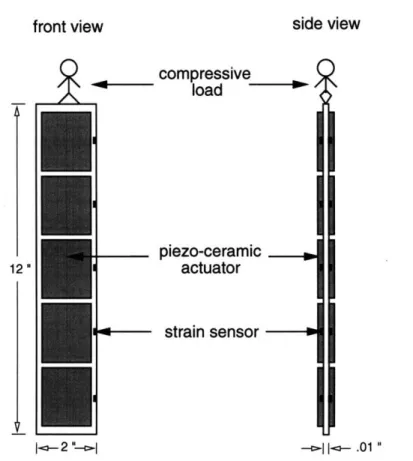
To demonstrate the feasibility of the approach, Berlin constructed a prototype actively controlled column, depicted schematically in figure 1-2 (see also figures 2-1-2-3 of chapter 2). The foot-long prototype column is a composite made of steel and piezo-ceramic materials. Arrays of strain sensors located along both sides of the column measure the dynamic state of the structure; similar arrays of piezo-ceramic actuators supply the control forces necessary to counteract buckling. Sensor mea-surements are supplied to a digital computer, which determines the desired control actions and sends the corresponding control signals to the actuators. The controller works essentially by estimating, given all of the latest sensor information, the current shape of the beam, and computing the control forces that would push the beam in

(10)

Figure 1-1: Buckling phenomenon in a real, full-scale structure. A 30-foot tall support beam buckled after being hit by a truck in a May 2, 1996 accident on Interstate 93 in Boston, Massachusetts ([8]). The steel beams are used to support the elevated section of the highway at the point where it crosses the Charles River.

(11)

front view 12 N v

compressive

load

II

-I piezo-ceramic actuator I

--strain

sensor

_ _ 1

II

I 2 " -- I - .01 "

Figure 1-2: Front and side views of Berlin's prototype actively controlled column subjected to a compressive load. The column is of length 12 inches, width 2 inches, and thickness 0.01 inches. Arrays of 5 strain sensors and 5 piezo-ceramic actuators are mounted on each side of the column. Sensor measurements are supplied to a digital computer (not shown), which calculates control signals to be sent to the actuators.

the direction of its undeflected position.

In his experiments, Berlin demonstrated an increase in the load-bearing strength of the prototype beam by a factor of 5.6. This result is very encouraging. Active control of buckling promises to enable us to create structures that are both stronger and lighter than the passive structures of today; taking this notion to an extreme suggests the possibility of building portable structures (e.g., portable bridges). Berlin suggests

a variety of possible other applications in [7, chapter 8]; they range from prevention

of metal fatigue in ships suffering from wave-induced whipping2, to building entire

cities on top of existing cities by making use of tall actively stabilized columns, an idea originally suggested by Zuk in [39].

2

This is a phenomenon in which compressive members supporting the hulls of large ships buckle in heavy sea conditions due to wave action pounding on the hull. While the duration of the offensive forces is usually too short to cause immediate failure, repeated whipping causes eventual metal fatigue ([7, p. 98]).

T

(12)

computational

unit

jiIIIIIIIIIIIIIIIMIMIIIIIIIIIIIIIMIIIIIn

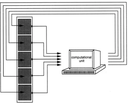
Figure 1-3: A system under centralized control. One computational unit collects all of the sensor information and directs control signals to all of the actuators.

1.1.2 Control Approaches

The type of controller Berlin uses to stabilize his beam is what we call a global, or

centralized, controller. The name refers to the control strategy's utilization of a global

model of the system, as well as global state information, to calculate control actions. Figure 1-3 contains a pictorial representation of a system under global control. All of the sensor information is directed to one centralized computational unit, which in turn sends control signals to all of the actuators. The computation of control forces is performed using knowledge about the dynamical behavior of the system as a whole, as well as the sensor information describing the state of the entire system.

Modern control theory is essentially the theory of centralized control: all tradi-tional control techniques assume both the existence of a global model for the system to be controlled, and the availability of global state information. These requirements make it difficult, in general, to apply traditional control techniques to active structural control, for two reasons. First, civil engineering structures tend to be too complex to allow for accurate modeling on a global scale. Secondly, the size and complex-ity of most real structures requires a great number of sensing sites, which makes it

practically impossible to collect all state information in a single place (i.e., the global

computational unit) and process it in a reasonable amount of time.

As an example, let us turn again to buckling control. As mentioned above, Berlin was able to prevent buckling of his prototype beam by using centralized control tech-niques. This was possible because, as we shall see in chapter 3, the global system dynamics of a simple structural element such as a beam can be modeled analytically; this immediately provides us with a global model to use as the basis for centralized control. In addition, the number of sensors and actuators required to control buckling

(13)

I..

L

I I

_

11F]_1

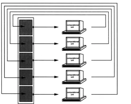
Figure 1-4: A system under decentralized control. The controller employs several computational units, each of which is responsible for controlling a small local region of the structure. In this example, a computational unit is provided for each sensor/actuator pair; the controller is truly local.

of a single beam is not prohibitively large; thus, all of the state information needed for determination of control actions can be collected and processed quickly and efficiently. On the other hand, consider applying full-scale buckling control to a complex structure such as a bridge, a ship, or an airplane-a massive structure composed of many (possibly heterogeneous) structural members. Interactions between the indi-vidual members composing such a structure are difficult to model accurately on a global scale. Furthermore, even if we could come up with a global model of such a structure, practical implementation of active control would require a very large num-ber of sensors. A single computational unit would simply not be able to interpret all of the state information quickly enough to be able to respond to it.

The above example demonstrates the need to develop control strategies that rely on neither the global models nor the global state information. We put such control strategies under the general label of decentralized control. As we envision them, decentralized controllers employ a multitude of computational units, each of which is responsible for controlling only a small local region of the entire structure. More precisely, each computational unit processes state information provided by the sensors located in its region, and generates control signals to the actuators in the region. Thus, there is no reliance on global state information in the determination of control actions. Furthermore, control signals are generated based purely on the local behavior of the system; no global models are utilized. Figure 1-4 demonstrates the decentralized approach, which should be contrasted with the centralized method of figure 1-3.

The main drawback of the decentralized control approach is that because of the lack of global information available in the computation of control actions, the overall control strategy implemented by a decentralized controller may not be globally

opti-I I I m ga Lm ! !

- -.;

I"' ~1~3 m

-

;-- ~5~ Imm

No

(14)

mal. The challenge faced by the control designer is to come up with a decentralized control strategy that retains global control authority, and thus yields effective global behavior.

In this thesis, we compare the centralized and decentralized control approaches for the specific case of a buckling beam. To prevent the beam from buckling, a centralized controller continuously estimates, given the global sensor information, the shape of the entire beam, and tries to push the beam in the direction of its undeflected position. Under local control, the beam is treated instead as a collection of small segments; for each segment, the controller determines, and tries to reduce, the local curvature. It is clear that both controllers, if successful, have the effect of keeping the beam close to the desired (straight) position, although the strategies employed are very different.

1.2 Related Work

Before diving into the details of the work performed in this thesis, let us briefly summarize prior work related to buckling control, as well as to centralized and de-centralized control methods.

1.2.1 Buckling Control

A good summary of work related to active control of buckling conducted prior to

Berlin's experiments is given in [7, chapter 2]. According to Berlin, "until recently, little attention has been given to the possibility of controlling buckling for the purpose of increasing the load-bearing strength of a structure" [7, p. 15]. Berlin was the first to demonstrate experimentally that the load-bearing capabilities of compressive members could be increased through active buckling control.

Berlin's experimental work was not limited to control of the prototype steel col-umn described above. To test the feasibility of active buckling control, Berlin first constructed a prototype column in which the control forces are applied by tendons at the midpoint of the column. A single pair of strain gauges was used to measure the curvature of the column at its midpoint. Through active control of buckling, the load-bearing strength of this simple prototype beam was shown to increase by a factor of 2. To demonstrate the possibility of incorporating more than one actively stabi-lized structural element into a structure, Berlin also constructed a railroad-style truss bridge with two compressive members controlled through the use of piezo-ceramic actuators. In addition to tendons and piezo-ceramic actuators, Berlin proposes a va-riety of other actuation strategies in [7, chapter 7], and suggests some applications in which these different strategies might prove useful.

In all of his experiments, Berlin employed a centralized approach to buckling control. In particular, his prototype steel column was controlled via "modal" control methods, introduced below. To our knowledge, no decentralized approach to active buckling control has previously been attempted.

(15)

1.2.2 Vibration Control

While control of buckling is a direction rather new in active structural control, there has been significant effort devoted to the study of vibration control. One of the main applications is active vibration suppression in flexible satellites and other large

spacecraft ([9], [31], [1], [29], [2], [5]); others include active damping of tall buildings

and active optics ([33]).

In some ways, active vibration control is similar to active control of buckling. Both types of controllers aim to minimize the motion of a structure away from its equilibrium position. However, in the case of vibrating structures, the equilibrium is stable; the job of the controller is to reduce the amplitude of oscillations. Structures undergoing buckling, on the other hand, are inherently unstable and will collapse if control is removed. In buckling controllers, then, there is much less tolerance for runtime failures and inaccuracies in the system model.

Another important point is that buckling control depends inherently on the actu-ator strength-the amount of force an actuactu-ator is capable of exerting. The greater the actuator strength, the more weight can be supported by an actively controlled structure. Limitations on actuator forces yield nonlinearities in the control strategy. Buckling controllers have to take these nonlinearities into account; we shall see the implications of this for buckling controller design in chapter 2.

Despite these key differences, many of the techniques developed in vibration con-trol are applicable to buckling concon-trol. These include both centralized and decentral-ized approaches, which we summarize below.

1.2.3 Centralized Control Strategies

The global approach that, over the last several years, has become the strategy of choice for control of large structures is independent modal space control (IMSC), introduced by Meirovitch ([22], [5], [33]). This method decouples the high-order dynamical sys-tem into a set of independent second-order syssys-tems, expressed in terms of "modal" coordinates. The control design is then carried out for each second-order system in-dependently. The resultant "modal forces" have to be transformed from the modal space to the actual control forces to be applied. We will be looking at IMSC much more closely throughout this thesis; from now on, we will refer to it simply as modal control.

Other common methods of centralized control, including pole allocation, linear optimal control, and nonlinear on-off control, are referred to as the "coupled" ap-proaches. These techniques were originally designed for systems in which the number of sensors and actuators is small relative to the plant dimension, and are not well-suited for control of large structures with multiple sensing and actuation sites. In [22], Meirovitch et al. show that IMSC holds many advantages over the coupled methods, which are more difficult to design and implement and require greater computational effort.

(16)

1.2.4 Decentralized Control Strategies

Most of the work on decentralized control has been done in the area of vibration control of large flexible space structures. A typical strategy is to decompose the system into a number of local subsystems, and to design individual controllers for each of the subsystems; any interactions between the subsystems are ignored. Examples of this approach can be found in [29], [38], [6], and [27]. In addition, there has been some theoretical work on establishing the robustness and stability characteristics of decentralized control methods ([12], [37], [36], [32], [16]). Many of the results pertaining to decentralized control techniques are summarized by Sandell et al. in [30]. The decentralized control techniques have been observed to work best for systems that can be naturally subdivided into lightly coupled subsystems. Strongly coupled structures, on the other hand, suffer from the lack of global control authority inherent in decentralized methods. In such systems, multilevel controllers have been used as

an alternative to purely decentralized designs ([30]). In this approach, control is

performed on both local and global levels. For example, Pitman and Ahmadian in [27] describe a multilevel design in which the local controllers are designed for performance, and the global controller is designed to minimize the coupling between the local subsystems. One disadvantage of this approach, however, is that it requires that the central controller have access to all the state information at the local level. More recently, Hall et al. ([13], [15]) presented a hierarchic control architecture in which control is achieved by a two-level combination of a centralized controller and a set of distributed residual controllers. The global controller handles the longer wavelength motions of the structure which cannot be effectively influenced by the local controllers, and only requires access to an aggregate of the local state information.

1.3 The Focus of This Work and New Results

As a first step toward exploring decentralized approaches to active control of buckling, this thesis investigates the viability of decentralized control as an alternative to cen-tralized control for the specific case of a buckling beam. Specifically, we compare two particular controllers, one centralized, another decentralized. The global approach used in our comparison is a modal (i.e., IMSC) controller. Our decentralized con-troller is what we call a purely local concon-troller: the control system is decomposed into

as many subsystems as there are sensor/actuator pairs3_{, and each actuator receives}

control signals based only on the readings of the associated sensor (see figure 1-4). In order to compare the performance of the modal and local controllers, we conduct qualitative analysis, simulation, and experimentation on a prototype beam. The results indicate that our local controller is capable of increasing the load-bearing strength of the beam to the levels comparable to those achieved through the use of

3In our system, there happen to be as many sensors as there are actuators; each sensor/actuator pair is collocated at some position along the beam. In general, the number of sensors and actuators may be unequal, in which case the definition of a local controller could be modified to include several sensors or actuators for each local subsystem.

(17)

25-

20-z

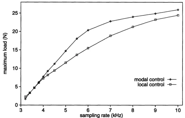
.9 15 E E E 10 E 5 0 3 4 5 6 7 8 9 10 sampling rate (kHz)

Figure 1-5: Simulation results comparing the performance of the modal and local controllers. The maximum load the beam is able to support (in Newtons) is plotted against the sampling rate of the controller (in kHz). The buckling load (i.e., the maximum load supported by an uncontrolled beam) for this beam is approximately 1.5 Newtons.

modal control. This is demonstrated in figure 1-5, which shows simulation results comparing the two control laws. One of the main factors influencing the amount of weight the actively controlled beam can support is the frequency with which the controller samples and responds to the state of the system; figure 1-5 shows the maximum load supported by the beam with respect to this sampling frequency. We can see from the plot that, although for the most part, the local control curve stays below the modal control curve, the local controller does not do much worse than the modal one. We will have much more to say about this particular plot, as well as the general limitations and advantages of each of our two controllers, in chapters 3 and 4.

The prototype beam employed in the experimental portion of this work is the beam built and used by Berlin in [7]. The results of the physical experiments indicate that the beam under modal and local control is able to support loads of 19.4 and 16.8 Newtons, respectively. With the maximum load supported by an uncontrolled beam measured at 5.3 Newtons, this translates into factors of 3.7 and 3.2 improvement

of the load-bearing strength of the beam achieved through active control.4 _{As in}

simulation, here again we observe a rather modest difference in performance of the two controllers.

These results indicate that the decentralized approach holds a promise for active control of buckling.

4

(18)

1.4 Overview

In the rest of this document, we describe the work leading to the main results outlined above, and provide a more detailed discussion of the results.

Chapter 2 supplies the general background for the rest of the thesis. We describe in more detail the experimental setup and the control system. We also motivate the choices made in controller design and implementation given the system at hand.

The main bulk of the thesis is contained in chapters 3-5. Chapter 3 reviews the dynamics of an axially-loaded beam under active control, and presents qualitative analysis comparing the modal and local controllers. In chapter 4, we describe com-puter simulations performed in order to evaluate the relative performance of the two control strategies, and discuss the results of these simulations. The experimental tests and results are presented in chapter 5.

Chapter 6 summarizes the main results obtained in this thesis, and suggests di-rections for possible future work.

(19)

Chapter 2 Setup

The purpose of this chapter is to provide the necessary background for the rest of the thesis. In particular, we describe the experimental setup which is taken as the basis for this work, and take a look at the control system and its components.

2.1 Experimental Apparatus

As mentioned in chapter 1, the experimental apparatus used in this thesis was origi-nally built by Berlin as part of the work described in his Ph.D. dissertation, [7]. Our experiments use all of the same hardware, which we briefly describe below; for more details, the reader is referred to [7, chapter4].

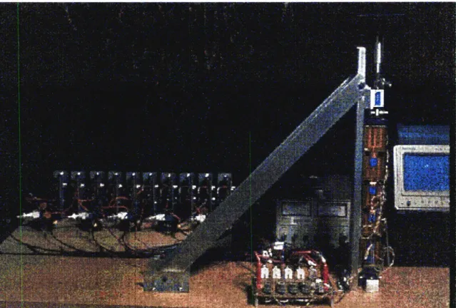
The apparatus used in the buckling control experiments is pictured in figure 2-1.1

The beam is held in a vertical position with the help of an assembly made of steel, planted on a wooden base. Wires run from the strain gauges on the beam to a circuit board located in front of the beam assembly, where the strain readings are amplified and passed on to the control computer. The equipment behind and to the left of the beam assembly consists of high voltage power supplies and amplifiers that accept control signals from the computer and use the amplified signals to drive the actuators. In what follows, we describe in more detail the beam assembly, and the principles behind sensing and actuation employed in the system.

2.1.1 Beam Assembly

The column in our experiment is designed to approximate a simply supported beam, meaning that the lateral displacement is zero at the two ends of the beam, but the ends are free to rotate. This condition is enforced by pinning the bottom end of the beam, and allowing the top end to move freely in the axial (vertical) direction. As shown in figures 2-2 and 2-3, two hinges are used to connect the ends of the beam to the rest of the beam assembly. The hinges hold the beam in a vertical position when

'The _{photographs of the experimental apparatus presented in figures 2-1-2-4 were taken by Philip}

Greenspun. Figures 2-1-2-3 originally appeared in Berlin's dissertation, [7]. They are reprinted here with permission of Andy Berlin.

(20)

Figure 2-1: Experimental apparatus, consisting of the beam assembly, the strain gauge amplifiers, and the high voltage power supplies and amplifiers which drive the actuators. Both sets of amplifiers are connected to the control computer, not shown here.

(21)

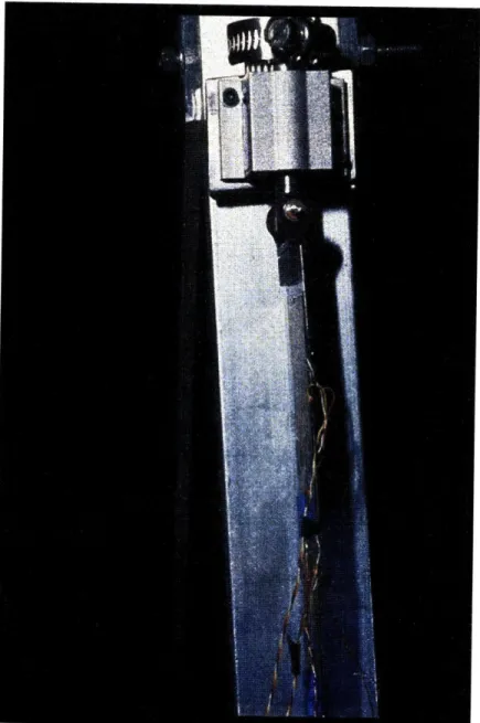
Figure 2-2: Front view of the prototype beam, subject to simply supported end conditions. The beam is connected to the assembly via a pair of hinges. A compressive load can be applied to the beam via a steel rod sliding vertically through a ball bearing. An aluminum clamp is placed on the rod above the ball bearing to prevent complete collapse of the column during buckling.

(22)

(23)

Figure 2-4: A closeup of the beam (view from the top). The column is covered with piezo-ceramic actuators. The gaps between the adjacent actuators are bridged by small 0.01 inch thick steel stiffeners.

(24)

no axial load is present, but allow it to bend under the influence of a compressive load. Lateral movement of the top and bottom of the column is prevented by connecting the hinges to two vertically aligned pin joints, which are held stationary in the horizontal direction. A compressive load is applied to the beam by placing it on top of a steel rod, which is allowed to slide up and down through a ball bearing (see figure 2-2). When the uncontrolled column is subjected to a load in excess of the critical load, the axial force thus applied pushes the rod down, resulting in the lateral bending of the column. In order to prevent the column from collapsing when buckling occurs, an aluminum clamp is placed on the rod slightly above the place where it passes through the ball bearing. The clamp acts to constrain the downward movement of the rod, thus guaranteeing the safety of the column.

The steel column has dimensions 12 inches by 2 inches by 0.01 inches (see figure 1-2). A closeup of the beam is shown in figure 2-4. Arrays of 5 strain gauges and 5 piezo-ceramic actuators are located on each side of the column. Each of the actuators is approximately 2.2 inches long and 1.75 inches wide. Thus, the actuators do not cover the entire length of the column; as can be seen from figure 2-4, there are small gaps (approximately 0.1 inches wide) between adjacent actuators. To prevent local bending of the column in these gaps, small 0.01 inch thick steel stiffeners are mounted between adjacent actuators.

2.1.2 Sensing

As we saw in figure 1-2, sensing in the system is provided by a total of 10 strain gauges. Each pair of strain gauges, located on the two sides of the beam, is used to measure the strain at one of the 5 points along the length of the beam. Two sensors rather than one are used at each point to provide for more accurate and reliable measurement: the value supplied to the control computer is actually the difference in

strains measured by the two sensors.

To h•b+ttr inrlar'at+ • nrli hn a; Ynificr-a"n ^fC -n +h 'n,' _

ments being taken by the sensors, consider a small segment of a deformed beam displayed in figure 2-5. The coordinate system associated with the beam is shown in the figure: x indicates the location along the length of the beam, while

y represents the deflection of the center of the beam (along

the column's thickness) away from the straight position. Let a be the thickness of the beam; then we observe that each of the two sensors is located a distance R awav from

the center of the beam.

Figure 2-5: Side view of a We assume in figure 2-5 that when the beam segment

deformed beam segment for a is deformed, the originally straight longitudinal lines turn

beam of thickness a. into arcs of circles (see [11, pp. 418-21]). The figure shows

the radii of curvature R, rl, and r₂of the arcs

correspond-ing to the center, the right side, and the left side of the beam, respectively. The angle

AO spans the arc segments 0102, A1A2, and B1B2 of interest. Notice that, in the figure, the arcs on the left side of the beam become longer, while those on the right

(25)

side become shorter as a result of the deformation. We assume that the length of the

centre arc 0102 stays equal to the straight line distance between the points 01 and

02 in the undeformed beam (see [11, pp. 424]).

Strain can be defined as the fractional change in the original length of a material; thus, the center of the column experiences zero strain, while the strain at the right end is given by

riAO - RAO

-!0A

a 1

fright 2

a

S= RA RAO 2 R

and similarly,

r2A - RAO a 1

fleft =

The difference in strain measured by the right and left sensors is then given by -ak, where - represents the curvature of the beam at the location of the sensors. For small deformations, curvature can be approximated by the second derivative of displacement (see [11, p. 514]), yielding the following expression for the difference in strain:

d2

s(x) = -ad2 (2.1)

We will make use of expression (2.1) in chapters 3 and 4, when discussing the control strategies used to prevent the beam from buckling.

2.1.3 Actuation

The actuators used in the experimental system are made of piezo-ceramic. When an electric field is applied to a ceramic material, it induces stress in the piezo-ceramic, causing it to either grow or shrink, depending on the polarity of the field. With a piezo-ceramic actuator mounted on the side of a column, application of an electric field results in forces being exerted on the beam by the actuators in an attempt to relieve the stress induced in the piezo-ceramic.

To be more specific, the actuation proceeds as follows. Given some control voltage

V, the corresponding electric fields of equal magnitude but opposite polarities are

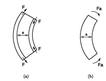
applied to the actuators on the two sides of the beam, causing one of them to grow and the other to shrink. This produces a longitudinal control force F applied at the endpoints of the actuators; F is tensile on one side of the beam, and compressive on the other (see figure 2-6a). The overall effect of the induced electric field is a pair of bending moments Fa (neglecting the actuator thickness), applied at the endpoints of the actuators; this is demonstrated pictorially in figure 2-6b.

As mentioned in chapter 1, an important parameter in active buckling control systems is the actuator strength-that is, the amount of force an actuator is capable

(26)

F

a

F

_FJ

Fa

(a) (b)

Figure 2-6: Actuation of a piezo-ceramic material mounted on the two sides of a beam. In (a), the actuator on the left side of the beam is growing, thus applying a tensile longitudinal force F to the left side of the beam segment, while the actuator on the right side of the beam is shrinking, yielding a compressive force F at the right end of the segment. The bending moments Fa produced

by these longitudinal forces are shown in (b).

of exerting. The piezo-ceramic actuators used in our experimental system can be subjected to voltages as high as 200 Volts; this corresponds to the maximum applied bending moments of roughly 0.14 Newton-meters.

Further details regarding the principles of piezo-ceramic actuation can be found in

[7, pp. 36-40]. For example, [7] explains the relationship between the applied voltage

V and the resultant actuator forces F, and discusses some nonlinear properties of the

piezo-ceramics.

2.2 Control System

The control system used in the active buckling control experiment is an example of

a closed-loop, or feedback system. Such a control system continuously compares the

actual state of the structure (the feedback signal) with the desired state, and uses the difference, or error, as a means of control. The aim of the controller is to reduce the error and bring the system to the desired state. In our case, the goal is to keep the beam in (or close to) its undeflected position, and the size of the error is measured by the magnitude of the beam's deflection away from that position. As we saw earlier in this chapter, the state of the structure is determined with the help of strain sensors, and the desired control forces are exerted by piezo-ceramic actuators. In addition to the forces induced by the actuators, the dynamics of the beam may be affected by external excitations (e.g., banging of a fist on the table).

A block diagram of the control system is depicted in figure 2-7. Here, the plant is

the uncontrolled system, represented by the transfer function G2(s). Its output X(s)

represents the state of the system. The actual state X(s) is fed back to a subtractor,

(27)

D(s)

X(s)

Figure 2-7: Block diagram of an active control system. The actual state of the plant X(s) is subtracted from the desired state R(s) to produce the error E(s). The controller with transfer function G1 (s) turns this error into a control action U(s), which is used to influence the dynamics of the plant. D(s) represents the external excitations affecting the behavior of the system, and G2(s) is the transfer function describing the dynamics of the plant.

which compares it to the desired state, R(s), and produces the error E(s). This error is acted upon by the controller with transfer function Gi(s) to produce the control action U(s), which, along with the external disturbance to the system D(s), forms the input to the plant.

Note that, in this chapter, we are being purposefully vague about what we mean by the "state" of the system. In general, there is more than one way to represent the system's state. For example, state in our system can be represented by a vector of 5 strain values measured by the sensors, plus their derivatives with respect to time. Another possibility is to base the control on the beam's deflection from the vertical (along with the derivative of the deflection); in this case, the sensor measurements have to be converted, via double integration (see equation (2.1)), to a measure of displacement. Thus, the state of the system is not necessarily measured by the sensors directly.

When we introduce modal and local control in chapter 3, we shall see that the two controllers employ two different representations of state. By not committing ourselves to any one state representation at the moment, we can talk about the high level issues in control system design and implementation regardless of the specific control approaches being used.

2.2.1 PD Control

Although the modal and local controllers employ different state representations, the control law transfer function Gi(s) used by the two controllers in our system is the same. This transfer function implements proportional plus derivative control, or sim-ply PD control. The main reason for choosing PD control from among a variety of control strategies available to a control designer is the simplicity of analysis and im-plementation that PD control provides. Berlin used a variant of PD control (what he termed "PIDV control") in his system ([7, pp. 54-9]) as well.

As indicated by its name, the action of a PD control law is composed of the response to the state of the system as well as its derivative. That is, the equation of

(28)

a PD controller is given by

de(t) (2.2)

u(t) = Pe(t) + D t(2.2)

where e(t) and u(t) are the input error signal and the controller output, respectively. In the frequency domain, the transfer function of a PD controller is thus

Gi~ _{) =}_E(s)Us = P + Ds

The constants P and D are termed the proportional and derivative gains, respectively.

The gains are chosen by the control designer such that the system exhibits the desired response for various kinds of inputs. We will have more to say about the process of gain selection shortly.

Intuitively, proportional control, in which the control action is proportional to the error, makes sense: if the error is large, a large corrective action is applied; if the error is small, a small corrective action is applied. Thus, proportional control tends to stabilize the system. Derivative control action, when added to a proportional controller, provides a means of obtaining a controller with high sensitivity. Derivative control responds to the rate of change of the actuating error and can produce a significant correction before the magnitude of the actuating error becomes too large. It thus helps prevent overshoot by anticipating the actuating error and initiating an early corrective action. One should note, however, that while high sensitivity of the derivative control gives the controller an anticipatory character, it also amplifies the high frequency noise present in the system. A more detailed discussion of PD control can be found in any control theory text, such as [23] or [19].

2.2.2 Determining Optimal Control Gains

It remains to specify the gains to be used in the PD control law. In modern control

design,2 _{control parameters are typically determined via pole placement or linear} optimal control (see [23, chapter 10], [33]). The idea behind these methods is to

identify a set of control gains that minimize some prespecified performance index. The

performance index provides a measure of how much the system's actual performance deviates from the ideal performance. For example, linear optimal controllers often employ quadratic performance indexes, which are quadratic functions of both the error signal and the energy required for control action, integrated over some period of time.

Calculating the control parameters which correspond to the minimal performance

index of this type requires solving the algebraic Riccati equation; several efficient solution methods are documented in the literature ([33]).

2

Modern control theory utilizes state-space methods, and is applicable to complex multiple-input, multiple-output systems. It was developed as an alternative to conventional control techniques which operate in frequency domain and are only applicable to single-input, single-output systems ([23]).

(29)

Like most control design techniques, modern control state-space methods are only applicable to linear time-invariant systems and yield linear control laws (hence the name "linear optimal control," for example). While all physical systems are nonlinear to some degree, most of them can be approximated as linear over a limited range of operation, and linear control techniques can still be used.

In buckling control, however, while the plant itself can be approximated by a linear system, the controller turns out to be inherently nonlinear. The difficulty stems from having actuators of limited strength. The actuators at hand may fall short of realizing the control signal u(t) for some time t, in which case the control signal has to be cut off, or saturated. Thus, actuator limits introduce nonlinearities in the control law. Because of these nonlinearities, optimal control gains for buckling controllers cannot be calculated via linear control methods directly.

Although all control systems involve actuators of finite strength, in most systems actuator limits are not of major concern. For example, vibration controllers can often be designed to have gains small enough that the desired control forces never exceed the actuator limits, thus avoiding the associated nonlinearities. This may handicap the controller somewhat, since it might not be using all of the available control authority; however, this usually has only a minor effect on the system performance. In buckling control, on the other hand, actuator limits directly affect the amount of weight the beam can support. A controller which is not using all of the control authority available to it will fail at loads smaller than it could have supported were it allowed to utilize the actuators to their fullest. Since the question of the maximum sustainable load is of major importance in this thesis, we cannot ignore the nonlinearities associated with limited actuator strength while calculating the optimal control gains.

Instead of using one of the state-space methods, we thus turn to numerical opti-mization techniques to compute the control gains. Numerical optiopti-mization routines still make use of a performance index, frequently termed the merit function. Op-timization consists of searching the space of variable controller parameters in order to find a point in the space where the merit function is minimized. The particular optimization technique we use is the downhill simplex method by Nelder and Mead, described in [28]. This method is extremely straightforward, and makes almost no special assumptions about the function to be minimized. The algorithm starts with an initial guess at the parameter values. At each step in the algorithm, the dynamics of the beam are observed for some specified period of time, and the merit of the control gains is evaluated using the performance index. The performance index employed is similar to the quadratic performance indexes used by linear optimal controllers: it is a quadratic function of both the deflection of the beam and the velocity with which the beam is moving, integrated over time. The beam's deflection indicates the magnitude of the error signal, while the velocity of the column provides a measure of kinetic energy present in the system. A more detailed description of this merit function, as well as the optimization process itself, is provided in chapter 4.

A major difficulty with this optimization approach is that the minima found by

the optimization routine may be local rather than global. We can use some ad hoc techniques to avoid getting trapped in local minima: for example, optimization can be performed several times, starting with different initial values of control gains, and the

(30)

best result among all the runs can be chosen. In addition, we can help the optimizer by picking "good" initial parameters by hand. Finally, optimization can be restarted at a point where it claims to have found a minimum; this may allow the routine to climb out of a local valley in which it might have gotten trapped (see [28, p. 410]).

With all these caveats, the optimization process can become rather computation-ally demanding and time-consuming. On the other hand, it provides a convenient, largely automatic way of obtaining optimal control gains for the system with nonlinear characteristics.

As a final note on optimization approaches, it is worth mentioning that the op-timization process described here is similar to the techniques used in optimalizing

control systems presented by Ogata in [23]. These systems exemplify adaptive

con-trollers, which seek to accommodate unpredictable environmental changes affecting the dynamics of a plant. For a plant experiencing large variations in environmental conditions (either within the system itself or external to it), it is usually not possible to design a single control law that would yield satisfactory system performance under all conditions. Thus, adaptive controllers have to continuously measure the dynamic characteristics of the plant and adjust the control parameters so as to compensate for changes in the plant dynamics. In optimalizing control systems, control parameter adjustment is performed based on an optimization routine much like the one described above. As Ogata points out in [23, p. 855], the greatest advantage of this approach is that no restrictions are placed on the plant: it can be nonlinear, time-varying, and so on.

Ultimately, of course, we would like the buckling controllers described in this thesis to be able to adapt to changes in environmental conditions. In the future, the optimization approach presented here may prove useful in the development of techniques for adaptive control of buckling.

(31)

Chapter 3 Qualitative Comparison

We are now ready for qualitative analysis of the system described in chapter 2. We start by deriving the dynamics of an axially-loaded beam subject to control forces. We then take a closer look at modal and local controllers, in particular. By the end of the chapter, we gain some insights into the system's behavior under both kinds of control, as well as the relative advantages and disadvantages of the two approaches.

3.1 Beam Dynamics

Consider a simply supported ideal beam of length L, width w, and thickness a, shown in figure 3-1. For simplicity, in the analysis of this chapter the beam is assumed to be uniform. The coordinate system associated with the beam is as indicated in figure 3-1. The beam is subjected to an applied axial load W, also shown

w in the figure.

In addition to the beam's physical dimensions, equations

y below involve the following material properties of the beam:

Young's modulus E, beam mass per unit length p, and area

moment of inertia I = wa3/12.

We assume that the length of the beam L is large com-pared to its width w and thickness a. When a short column is put under a gradually increasing compressive load, it even-tually fails by crushing. When the column is long, however, it will fail by buckling, that is, by bending and deflecting lat-erally, rather than failing by direct compression, at a load W very much smaller than is required to crush the material.

Typically, the buckling phenomenon is explained by an-alyzing the stability properties of a loaded beam in static

eauilibrium (see [14]. [111. and

r341).

It can be shown that if

W _{the axial load W is below a certain critical value, termed the}

Figure 3-1: A simply buckling load, the system is in stable equilibrium-that is, if supported ideal beam un- the beam is disturbed, it will return to the straight position

der an axial load, W. _{once the disturbing force is removed. As W is gradually}

(32)

creased, a condition of neutral equilibrium is reached when W is equal to the buckling load; at this load, the beam may theoretically have any small value of deflection, and a small lateral force will produce a deflection which does not disappear when the force is removed. At loads higher than the critical load, the beam is unstable and will collapse. The value for the buckling load can be obtained by solving the differential equation governing the deflection of the beam in static equilibrium.

Instead of taking the static approach, however, we study buckling behavior by considering the dynamics of a beam in motion. In practice, a slender column such as the one in figure 3-1 is subject to many perturbations induced by the environment, and is thus never perfectly still. By studying beam dynamics, we will be able to understand and predict the response of the beam to external forces and perturbations, explain the origins of buckling, and come up with ways to prevent the buckling behavior.

Below, we first gain some insight into the natural response of the system to per-turbations, by taking a look at free vibration of an unloaded beam. We then discuss how applying an axial load changes the dynamics of the beam and introduces a po-tential for instability. Finally, we consider the effects of applying control forces aimed to stabilize the beam's vibrations, thereby preventing its collapse.

3.1.1 Free Vibration

Suppose an unloaded beam is initially at rest in its equilibrium position-i.e., the straight position, y(x)= 0. At time t= 0, some external force is applied to the beam, causing a deflection away from the original equilibrium. If the external force is then removed, the beam will vibrate; such motion is called free vibration.

Because w < L, we assume that the deflection y of any point on the beam depends only on its location x along the length of the beam and on time t, and not on its position along the width of the beam. The equation of motion of the beam is thus a partial differential equation which describes how the displacement y varies with respect to x and t.

In order to obtain the equation of motion of a vibrating beam, we take a look at the forces and bending moments applied to an infinitesimal segment of the beam (considered as a free body), pictured in figure 3-2. The segment is located at a distance x from the left end of the beam (oriented horizontally for convenience), and is of length dx; the time-varying lateral displacement of the segment is given by y. Applied at the two ends of the segment are the shear forces V(x, t) due to the adjacent segments of the beam, and the bending moments M(x, t) associated with the beam's deflection. If we designate the shear force at the left end of the segment by V, and the bending moment by M, then the corresponding quantities at the right end can be expressed as V + L-fdx and M + Odx. Finally, the acceleration of a vibrating

beam segment is given by -2, resulting in an inertial force p dx in the negative y

direction.'

For our system to be in dynamic equilibrium, both forces and moments must be balanced about an arbitrary point on the beam ([35, p. 241]). Applying these 'See [11, pp. 158-60] for a more detailed derivation of the equations associated with figure 3-2.

Active control of buckling : centralized and decentralized approaches

Active Control of Buckling:

Centralized and Decentralized Approaches

by

Natalya Cohen

JUN

111996

:ertified by

,

Active Control of Buckling:

Centralized and Decentralized Approaches

by

Natalya Cohen

Abstract

Acknowledgments

Contents

List of Figures

List of Tables

Chapter 1

Introduction

1.1

Background: Active Structural Control

1.1.1

Active Control of a Buckling Beam

compressive

load

II

--strain

sensor

II

T

1.1.2

Control Approaches

L

_

11F]_1

- -.;

-

No

1.2

Related Work

1.2.1

Buckling Control

1.2.2

Vibration Control

1.2.3

Centralized Control Strategies

1.2.4

Decentralized Control Strategies

1.3

The Focus of This Work and New Results

20-z

1.4

Overview

Chapter 2

Setup

2.1

Experimental Apparatus

2.1.1

Beam Assembly

2.1.2

Sensing

riAO - RAO

-!0A

a 1

a

2.1.3

Actuation

F

F

FJ

2.2

Control System

2.2.1

PD Control

2.2.2

Determining Optimal Control Gains

Chapter 3

Qualitative Comparison

3.1

_FJ