Contributions to the anisotropic elasto-plastic analysis of shells

Contributions to the Anisotropic Elasto-Plastic

Analysis of Shells

by

Do-Nyun Kim

Bachelor of Science in Mechanical and Aerospace Engineering

Seoul National University, February 2000

Master of Science in Mechanical and Aerospace Engineering

Seoul National University, February 2002

Submitted to the Department of Mechanical Engineering

in partial fulfillment of the requirements for the degree of

Doctor of Philosophy in Mechanical Engineering

at the

MASSACHUSETTS INSTITUTE OF TECHNOLOG

ARCHIVES

JUN 16 2009

LIBRARIES

June 2009

©

Massachusetts Institute of Technology 2009. All rights reserved.

Author ...

...

Department of Mechaiical Engineering

May 16, 2009

Certified by...

Klaus-Jiirgen Bathe

A ofessor of Mechanical Engineering

,/

A

0/

j~is Supervisor

Accepted by ...

...

David E. Hardt

Chairman, Department Committee on Graduate Students

Contributions to the Anisotropic Elasto-Plastic Analysis of

Shells

by

Do-Nyun Kim

Submitted to the Department of Mechanical Engineering on May 16, 2009, in partial fulfillment of the

requirements for the degree of

Doctor of Philosophy in Mechanical Engineering

Abstract

Shells are probably the most widely used structural component in engineering and also in nature due to their high efficiency and excellent performance when properly designed. On the other hand, they can be very sensitive to changes in geometries, thicknesses, applied loads and boundary conditions. Hence much research effort has been devoted to the reliable and efficient analysis of shells. This work contributes to the anisotropic elasto-plastic analysis of shells by addressing key issues in developing shell elements for finite element analysis and an elasto-plasticity model considering anisotropy and its evolution.

First we develop a shell element that models the three-dimensional (3D) effects of surface tractions. The element is the widely used MITC4 shell element enriched by the use of a fully 3D stress-strain description, appropriate through-the-thickness displacements to model surface tractions, and pressure degrees of freedom for incom-pressible analyses. The element formulation avoids instabilities and ill-conditioning.

We also develop a triangular 6-node shell element that represents an important improvement over a recently published element. The element is spatially isotropic, passes the membrane and bending patch tests, contains no spurious zero energy mode, and is formulated without an artificial constant. In particular, the improved element does not show the instability sometimes observed with the earlier published element. Finally we review a constitutive model for anisotropic elasto-plastic analysis which takes into account the anisotropy of both the elastic and plastic material behaviors, as well as their evolution with plastic strains. It is based on continuum energy con-siderations, the Lee decomposition of deformations and a stored energy function of the logarithmic strains. The present work focuses on giving some physical insight into the parameters of the model and their effects on the predictions in proportional and in non-proportional loading conditions.

Thesis Supervisor: Klaus-Jiirgen Bathe Title: Professor of Mechanical Engineering

Acknowledgments

Thank God, my father in heaven, for giving me a wonderful opportunity to study at MIT and meet great people. You always leads me and my family into the right path. May your name be honored.

I would like to thank my thesis supervisor, Prof. Klaus-Jiirgen Bathe, for his excellent support and encouragement throughout my doctoral research. His insight and passion for research and teaching have led me to the right places. In particular, he inspires me to be happy at myself, my work and my life under any circumstance.

I am thankful to my committee members, Prof. Tomasz Wierzbicki and Prof. Eduardo A. Kausel, for their valuable comments and suggestions. I am grateful to Prof. Francisco J. Montns for his collaboration in anisotropic elasto-plasticity models and to Prof. Phill-Seung Lee for sharing his experiences in developing triangular shell elements.

I would also like to thank my colleagues in the Finite Element Research Group at MIT, Jared Craig Ahern, Samar Malek, Reza Sharifi Sedeh, Haining Zheng, and Christian Deilmann, for their help, encouragement and friendship. I appreciate help and friendship of Korean graduate students in MechE and Aero-Astro at MIT.

I am very thankful to friends and families in First Korean Church in Cambridge and especially to all those who have prayed for me even without knowing who I am. I acknowledge that this work has been partially supported by Korea Science and Engineering Foundation and by John Oak Scholarship.

My utmost gratitude is due to my family. My special thanks go to my parents and brother for their endless love, support, encouragement and prayer whatever I do. I am also truly grateful to my parents-in-law and brothers- and sister-in-law for their priceless support and prayer. Special thanks are due to my precious daughter and son, Yeji and Yeil, for cheering me up through their world best smiles. I would like to give my last and most valuable thanks to my wife, Hye-Lim, for her unconditional love, sacrifice, trust, support and encouragement.

Contents

Introduction 17

1 A 4-node 3D-shell element to model shell surface tractions and

in-compressible behavior 19

1.1 The shell model ... ... 21

1.2 Finite element discretization . ... . . . 27

1.2.1 Interpolation of geometry and displacement . ... 27

1.2.2 Mixed interpolation of strain field . ... 28

1.2.3 Displacement/Pressure (u/p) formulation . ... 29

1.3 Numerical studies . . . ... ... 30

1.3.1 Cantilever beam under in-plane tangential tractions on the top and bottom surfaces ... ... ... ... . 30

1.3.2 Pressurized cylinder . ... .... 33

1.3.3 Test cases for conditioning of the stiffness matrix ... 40

1.3.4 Hyperboloid shell problems . ... 43

1.3.5 A quadrant of a cantilevered cylinder under in-plane tangential tractions ... ... . ... 46

1.4 Concluding remarks ... ... ... 51

2 A triangular 6-node shell element 53 2.1 The formulation of the MITC6 shell element . . . ... . . 57

2.2 The improved MITC6 shell element .. . . . . . ... . . 60

2.3.1 Analysis of clamped plate problem ... . .. 64

2.3.2 Analysis of cylindrical shell problems . ... 65

2.3.3 _{Analysis of hyperboloid shell problems . ... . 65}

2.3.4 A brief study using a stabilized shell element formulation . . . 71

2.4 Concluding Remarks ... .... . 77

3 A model for large strain anisotropic elasto-plasticity ₇₉ 3.1 The Montans-Bathe model . ... . . . . 82

3.1.1 Kinematics ... _{. 82}

3.1.2 Dissipation inequality ... .. . . 84

3.1.3 Yield functions . ... . . . . . 86

3.2 Parametric study ... ... .. . 88

3.2.1 Constitutive equation for spin tensors . ... 88

3.2.2 _{The direction of axes rotation through elastic anisotropy} . . . 90

3.2.3 Sensitivity of the spin parameters . ... 91

3.3 Identification of spin parameters based on the R-values .. ... 98

3.4 Predictability of the model in multi-paths loading problems ... 104

3.5 Concluding Remarks ... .... ... . 109

Conclusions ₁₁₅

A The analytic solution for the cantilever beam subjected to in-plane

tractions ₁₁₇

B Mapping tensors from quadratic to logarithmic strain space 121

List of Figures

1-1 Shell geometries in the initial and deformed configurations. ... 23

1-2 The quadratic and cubic displacement functions at node k. ... 23

1-3 Stress distributions in a cantilever beam under in-plane tractions (Case

1) ... ... . 34

1-4 Stress distributions in a cantilever beam under in-plane tractions (Case

2) ... ... . 35

1-5 Stress distributions in a cantilever beam under in-plane tractions (Case

3).. ... . ... .... .... 36

1-6 Pressurized cylinder in plane strain condition; 0 = 2 °, Pi = 20t, Po =

80t, R = 10.0, E = 1.0x 104; (a) the whole model, (b) single element

representation (only radial displacement is allowed) . ... 37 1-7 Stress distributions in the pressurized cylinder (t = 0.1, Pi = 2.0, Po =

8.0) ... .. 38

1-8 Stress distributions in the pressurized cylinder (t = 2.0, Pi = 40, Po =

160) ... . . ... ... 39

1-9 Single element test for ill-conditioning; (a) director vectors are nor-mal to the mid-surface, (b) director vectors are rotated 30 from the

normal direction . ... .. ... 40

1-10 Eigenvalues of single element (11-DOF, E = 1.0 x 107, v = 0.3, t = 0.1) 41 1-11 Eigenvalues and condition numbers (director vectors are normal to the

1-12 Eigenvalues of single element in almost incompressible case (11-DOF,

E = 1.0 x 107, v = 0.499999, t = 0.1); director vectors are normal to

the mid-surface ... ... . 43

1-13 The hyperboloid shell problem (E = 2.0 x 1011,t = 0_.0 1_{,po = 1.0 x 106) 44} 1-14 The quadrant of a cantilevered cylinder under in-plane tractions (E =

1.0 x 104, V = _{0.3, length=40, thickness=0.1); (a) case of applied}

longitudinal traction (q = 0.1), (b) case of applied circumferential

traction (q = 0.007) ... ... 46

1-15 The deformed shapes when the traction is applied in the longitudinal

direction ... ... ... 47

1-16 Displacement in z-direction of point A in Fig. 1-14(a) ... 47 1-17 The effective stresses on the top and bottom surfaces in Case (a) of

Fig. 1-14 ... ... .... ... ... 48

1-18 The deformed shapes when the traction is applied in the circumferential

direction ... ... ... 49

1-19 Displacement in z-direction of point B in Fig. 1-14(b) ... 49 1-20 The effective stresses on the top and bottom surfaces in Case (b) of

Fig. 1-14 ... ... ... 50

2-1 Interpolations and tying points used for the MITC6 shell element; rl =

1 = 1 1

s1 r2 = S2 22v- andr 3 = s3 ... 60

2-2 Analysis of a hyperboloid shell problem. The midsurface is given by

2 +z 2 = 1+y 2 _{(-1 < y < 1). The shell is fixed at its bottom}

and free at its top; E = 2.0 x 1011, v = 1/3, t/L = 1/10000 (where

t denotes the thickness of the shell, see Sec. 2.3); the loading is the pressure loading p(O) = po cos(20), Po = 1.0 x 106. The problem is solved using the original MITC6 shell element of Ref. [1]. ... . 61 2-3 Isotropic element test of the 6-node triangular shell element, taken

from Ref. [1] ... ... ... 63

2-5 Shell problem of Fig. 2-2 solved with the improved MITC6 shell element 65

2-6 Clamped plate subjected to uniform pressure; L = 1.0, E = 1.7472 x

107, v = 0.3 and q = 1.0 ... .. ... 66

2-7 Convergence curves for the clamped plate problem. The bold line shows the optimal convergence rate. . ... . . 66

2-8 Cylindrical shell problem; pressure loading p(0) = po cos(20); both ends

are either clamped or free, see Refs. [1, 2]; L = R = 1.0, E = 2.0 x 105,

v= 1/3 and po = 1.0 ... ... ... 67

2-9 Convergence curves for the cylindrical shell problem (a) when both ends are clamped and (b) when both ends are free. The bold lines show the optimal convergence rate. . ... 68

2-10 Meshes used for 1/8th of the hyperboloid shell (8 x 8 element mesh) with symmetry boundary conditions applied. The geometry, material properties and loading are as in Fig. 2-2. (a) The graded mesh is used when both ends are fixed and (b) the uniform mesh is used when both ends are free. The boundary layer of width 6v/t is meshed in the graded

mesh [1] ... ... ... . 69

2-11 Convergence curves for the hyperboloid shell problem (a) when both ends are clamped and (b) when both ends are free. The bold lines show the optimal convergence rate. ... ... 70

2-12 Convergence curves in the Am norm for the fully clamped hyperboloid shell problem solved using (a) the displacement-based 6-node element, (b) the original MITC6 element and (c) the improved MITC6 element. Graded meshes are used as shown in Fig. 2-10(a). . ... . . 72

2-13 Convergence curves in the Am norm without shear terms for the fully clamped hyperboloid shell problem solved using (a) the displacement-based 6-node element, (b) the original MITC6 element and (c) the improved MITC6 element. Graded meshes are used as shown in Fig.

2-14 Rotation magnitudes

(Va

ele-ment. (a) C = 0.1, (b) C = 0.2 and (c) C = 0.4 . ... . . 76 3-1 The evolution of the principal orthotropic directions at different spatial

strains ex _{when uniaxial tensile loading is applied to a metal sheet}

along the x-axis. 0 is the angle between the rolling direction and the

loading direction (x-axis). Three initial orientations (300, 45 and

60 o) of orthotropic axis are considered. See Refs. [3,4] for the detailed description of the experiment and the analysis. The other material parameters are listed in Table 3.1. ... 90 3-2 The effect of the elastic anisotropy. (a) The evolution of the

prin-cipal orthotropic directions, (b) Young's modulus at different angles with respect to the rolling direction (a-direction). Ea = 204GPa and Eb = 203GPa are used for the solid lines while E, = 203GPa and Eb = 204GPa are used for the dashed lines where a and b represent

the rolling direction and the transverse direction of a metal sheet re-spectively. See Table 3.1 for the other elastic constants which are the

same for both cases. ... ... 92

3-3 The effect of the elastic anisotropy. (a) The evolution of the principal orthotropic directions, (b) Young's modulus at different angles with

respect to the rolling direction (a-direction). Ea = Eb = 204GPa. . . 93

3-4 The effect of the elastic anisotropy. (a) The evolution of the principal orthotropic directions, (b) Young's modulus at different angles with respect to the rolling direction (a-direction). Ea = 214GPa and Eb =

3-5 The effect of the elastic anisotropy. (a) The evolution of the principal orthotropic directions, (b) Young's modulus at different angles with respect to the rolling direction (a-direction). Ea = 212GPa and Eb =

214GPa ... . ... . ... 95

3-6 The effect of parameters on the evolution of the principal orthotropic directions. 0 is the initial orientation of orthotropic axis ... 97

3-7 Contour maps for ) with respect to p and r. (a) m = 1, (b) m = 2. The dashed lines represent where the change of 4 is minimum. ... 99 3-8 The evolution of the orthotropic axis and the flow stresses. Pairs of p

and r7 on the dashed line in Fig. 3-7(a) are used with m = 1 .... . 100 3-9 The evolution of shear stress in a reverse simple shear test (m = 1) (a)

with pairs of p and q shown as the dashed line in Fig. 3-7(a); (b) with the fixed p = 0.204; (c) with the fixed rI = 40. . ... 101 3-10 The evolution of flow stresses and R45 for DDQ-1 in Table 3.2. The

experimental results are taken from Ref. [5] . ... 105 3-11 The evolution of flow stresses and R45 for DDQ-2 in Table 3.2. The

experimental results are taken from Ref. [5] ... 106 3-12 The evolution of flow stresses and R45 for DQ in Table 3.2. The

ex-perimental results are taken from Ref. [5] . ... 107 3-13 The multi-paths loading problems. (a) Initial configuration where a

and b represent the rolling direction and the transverse direction of a metal sheet respectively; (b) The case of monotonic simple shear; (c) The case of reverse simple shear; (d) The case of tension-shear . . . . 108 3-14 Multi-path loading response (without plastic spin); (a) isotropic

hardening model - neither 'cross' nor 'Bauschinger' effect, (b) mixed hardening model - no 'cross' but 'Bauschinger' effect. (M = 0.9 and H = D where D is the fourth order deviatoric projection tensor) . . . 110

3-15 Multi-path loading response (with plastic spin); (a) isotropic hard-ening model - 'cross' but no 'Bauschinger' effect, (b) mixed hardening

model - 'cross' and 'Bauschinger' effect. (M = 0.9 and H = ID where

ID is the fourth order deviatoric projection tensor) . ... 111 3-16 The effect of the amount of prestraining on crossing. (Isotropic

hard-ening, M = 1.0) ... ... .. 112

3-17 An effect of the mixed hardening parameter (M) on the cross effect. (hE = hE = 1.2, hE _{= 0.6, = h = h = 0.5) . . . . . .}

List of Tables

1.1 The components of the linear incremental displacement given in Eq. (1.11) 27

1.2 Summary of shell models ... ... 31

1.3 Cases of applied tractions and analytic stress distributions for the in-plane traction test ... ... . 32

1.4 Normalized radial displacement of the pressurized cylinder at r = R . 37 1.5 CK with different element thicknesses, see Fig. 1-9 (E = 1.0 x 107, v = 0.3)... ... ... ... 41

1.6 The clamped-clamped hyperboloid shell (v = 0.333333) ... 45

1.7 The clamped-clamped hyperboloid shell (v = 0.499999) ... 45

1.8 The free-free hyperboloid shell (v = 0.333333) . ... 45

1.9 The free-free hyperboloid shell (v = 0.499999) ... 45

2.1 Basic test results of MITC6 shell elements . ... . 63

2.2 Normalized maximum displacements of the clamped plate problem in Fig. 2-6 ... ... ... 77

3.1 The material parameters used in Sec. 3.2 . ... 91

3.2 The material parameters used in Sec. 3.3 . ... 104

Introduction

Thin-walled structures or shells are well recognized as a basic building block found abundantly in nature ranging from small to large scale systems. Shells carry applied loads in an impressively effective way while securing a relatively large space inside them in spite of their thinness and lightness.

Shells are probably the most widely used structural component in engineering practice. They, when properly designed, provide a comparatively light and large structure that can hold applied loads very effectively with a small amount of materials, i.e. at a low cost. However shells, especially thin shells, can be extremely sensitive to imperfections and changes in geometries, thicknesses, applied loads and boundary conditions. Hence a reliable analysis is the key to design an effective shell structure. To a large extent, shell structures are now solved in practice using finite element procedures since it is almost impossible to obtain solutions analytically when the geometry and boundary conditions of shells are not simple. The finite element analysis of shells has now matured to the extent that it sometimes seems any complex shell can be accurately analyzed. In fact, however, there are still a number of outstanding difficulties. These relate to the development of more effective shell finite elements, the design of better contact algorithms to accurately model frictional forces applied on a shell's top and bottom surfaces, as needed for example in metal forming analysis, and the development of better constitutive models for existing and new materials, just to name a few only.

The present work focuses on the anisotropic elasto-plastic analysis of shells by addressing key issues in obtaining improved shell elements for finite element analysis and an elasto-plasticity model considering anisotropy and its evolutions.

In chapter 1, we present a shell element that models the three-dimensional (3D) effects of surface tractions, like needed when a shell is confined between other solid media. The element is the widely used MITC4 shell element enriched by the use of a fully 3D stress-strain description, appropriate through-the-thickness displacements to model surface tractions, and pressure degrees of freedom for incompressible analyses. The element formulation avoids instabilities and ill-conditioning. Various example solutions are presented to illustrate the capabilities of the element.

In chapter 2, we present a triangular 6-node shell element that represents an important improvement over a recently published element [1]. The shell element is formulated, like the original element, using the MITC procedure. The element has the attributes to be spatially isotropic, to pass the membrane and bending patch tests, to contain no spurious zero energy mode, and is formulated without an artificial constant. In particular, the improved element does not show the instability sometimes observed with the earlier published element. We give the convergence behavior of the element in discriminating membrane- and bending-dominated benchmark problems. These tests show the effectiveness of the element.

In chapter 3, we review a constitutive model for anisotropic elasto-plastic analysis which takes into account the anisotropy of both the elastic and plastic material behav-iors, as well as their evolution with plastic strains. The model is based on continuum energy considerations, the Lee decomposition of elastic and plastic deformations and a stored energy function of the logarithmic strains. We give some physical insight into the parameters of the model and their effects on the predictions in both proportional and in non-proportional loading conditions.

Chapter 1

A 4-node 3D-shell element to

model shell surface tractions and

incompressible behavior

The finite element analysis of shells has now matured to the extent that it sometimes seems any complex shell can be accurately analyzed. In fact, however, there are still a number of outstanding difficulties. These relate to the more accurate modeling of shell structures to include 3D effects, the development of still more effective shell finite elements, in particular triangular elements, and the mathematical analyses to ensure optimality of the finite element solutions [2, 6]. To a large extent, shell structures are now solved in practice using 4-node shell elements. Among those available, the MITC4 shell element is probably the most effective element, in particular when linear and nonlinear analyses are to be performed [2,6-10]. However, the other MITC shell elements can be more effective for specific analyses [1,9, 11, 12].

The formulation of the MITC4 shell element is based on the Reissner-Mindlin assumptions of "material fibers originally straight and normal to the shell mid-surface do not stretch and remain straight" and "zero stress normal to the shell mid-surface" [2,6]. The MITC elements can be formulated using a continuum rep-resentation or the 'basic shell model' identified by Chapelle and Bathe [2, 6, 13, 14]. While the Reissner-Mindlin assumptions are widely applicable, they cannot model

the application of shell surface stresses as needed in the analysis of a shell confined between solid media. For example, in metal forming, the normal and shear trac-tions applied to thin sheet surfaces can be large and the accurate modeling of normal stresses and shear stresses can be important. Of course, in addition, large strain elastic-plastic (almost incompressible) conditions need be represented.

To model the effects of surface tractions, it appears that 3D shell-solid elements are most appropriate, see [15-19] and the references therein. In the formulation of these elements, the top and bottom surfaces of the shell are represented geometrically

and their positions are updated through the displacement degrees of freedom, just like in a fully 3D analysis of solids but with only one element layer through the shell thickness [2, 6]. Since the bending strains vary linearly, clearly, for consistency with bending theory including the Poisson ratio coupling, the through-the-thickness normal strain must also be allowed to vary linearly. This requires a quadratic interpolation of displacements through the shell thickness. The shear, membrane and pinching locking can be relieved using MITC strain interpolations.

While sometimes effective, these elements display severe ill-conditioning when the shell becomes thin and when the shell is an (almost) incompressible medium [20,21]. To improve the element behavior and computational effectiveness, instead of dis-placement degrees of freedom, enhanced strains have been used, see for example Refs. [15, 22,23], and the references therein. However, enhanced strain formulations can be unstable, see Refs. [24,25], and are therefore best avoided. Hence, a more effec-tive approach is to build on the basic MITC4 shell element, for which all shell actions are represented using the shell mid-surface, use the three-dimensional stress-strain description, and enrich the shell element formulation 'judiciously' by appropriate dis-placement and pressure interpolations. These interpolations need to be selected to not introduce instabilities or ill-conditioning. This approach was used in Ref. [26] to enrich the MITC4 shell element by two element degrees of freedom corresponding to thickness stretching (a constant and a linear term) in order to represent large strain effects.

3D stress-strain law, and by displacements and pressure used to represent accurately the effects of shell surface normal and tangential tractions, and incompressible con-ditions. The enrichment in displacements is achieved by simply adding displacement interpolations with corresponding degrees of freedom at the 4 nodes. The result-ing displacements are compatible across element boundaries. To render the element also applicable to (almost) incompressible conditions, the u/p formulation with an assumption on the pressure is used [6]. All these degrees of freedom, including the pressure degrees of freedom, can be invoked hierarchically as desired. This hierarchi-cal feature of the element is very attractive, obviously from a modeling point of view, but also from a practical point of view. Namely, the pre- and post-processing capa-bilities of the classical MITC4 element are directly applicable by simply increasing the number of degrees of freedom allowed for the element.

The element presented in this chapter is largely based on concepts previously published but in this chapter we have synthesized various ideas in an aim to obtain an overall effective formulation. In particular, this 3D-shell element formulation does not show ill-conditioning. In the following sections, we first present the formulation of the continuum shell model, then the finite element discretization, and finally we give the results of various illustrative example solutions.

1.1

The shell model

In this section, we present the shell model that we will solve by our finite element discretization. We follow the notation used in Ref. [6].

The initial geometry at time 0 is described by

X=_4 oa o (1.1)

2

where ( is the natural coordinate in the thickness direction, 0_{YM is the position vector} of material particles in the shell mid-surface, oa is the thickness and OVn is the director

In the deformed configuration, an initially straight fiber may be curved with the assumption shown in Figs. 1-1 and 1-2. The assumed deformed geometry at time t is

X= XM+- ₂ a + 2 oa t tVn

+ ±2 0_{a (tQj il + t2 ) (1.2)}

+_3 0 (tC 1 t 1 +t 2 V2)

Here tn is the director vector at time t, ta is the shell thickness at time t, til and tV2

are are unit vectors orthogonal to tVn and to each other, tQn is the degree of freedom corresponding to a quadratic displacement function in the direction tVn, and tQ, and

tC, represent degrees of freedom corresponding to quadratic and cubic displacement

functions in the directions tV, with a = 1, 2. The left superscripts 0 and t always denote that a quantity is given at time 0 and t. With these assumptions, the fiber originally normal to the mid-surface can strain linearly and become curved, and the transverse shear stresses have a quadratic distribution through the shell thickness. This enables the element to precisely capture the effect of in-plane tractions, like normal and frictional forces, applied on the top and bottom shell surfaces. Note that

oa, the initial thickness, is employed in front of each higher order function. This is

a scaling factor in order to avoid ill-conditioning of the global stiffness matrix as the thickness becomes small. It is more natural to use the current thickness but we use the initial thickness because this leads to a simpler formulation.

In the same way, the deformed geometry at time t + At is defined by

X t+a t = XM t+t t+t + 2 0a t+AtQn t+Atn

2

+~2 0a (t+AtQ1 t+Atl + t+AtQ2 t+At2) (1.3)

+ 3oa (t+AtC1 t+AtV + t+AtC2t+t)

dis-t k

V2

Figure 1-1: Shell geometries in the initial and deformed configurations.

t k t nk _{t nk}

n 94

Figure 1-2: The quadratic and cubic displacement functions at node k. tv-k

placement field as follows.

= t+t - t = t+At - t

U = U- U = X- X: (1.4)

Then we have

-= (t+At -

)

V)

20 t+tQ1t+At _{tQ t) + 2 Oa (t+AtQ t + 2 t2}

t )

+ (3 a (t+ + +C At' Ct_ 1 ) + 3 a (t+AtC2 t+At tC 2 )

(1.5) This field can be expressed in terms of degrees of freedom at time t for the incremental displacements using the following relations.

t+At- t-. XM _ XM = UM t+Ata _{_ t} a = Oa -Aa t+AtQn _ tQ = q, t+AtQ1 - tQ 1 = ql t+AtQ - tQ2 =q2 t+Atc1 - tC_{1 = c} 1 t+tC 2 - tC₂ = C₂ = ui + ve2 + w, ₃

Here Eq. (1.6a) represents three translations in the global Cartesian coordinate system given by the unit vectors Fei, with i = 1, 2, 3, Eq. (1.6b) gives a thickness change and Eqs. (1.6c)-(1.6g) define displacement increments. Note that, in Eq. (1.6b), the incremental thickness change is normalized by the initial thickness to circumvent ill-conditioning.

For the shell element, two rotational degrees of freedom have been generally used to describe the rotation of a director vector. We, instead, adopt three rotational (1.6a) (1.6b) (1.6c) (1.6d) (1.6e) (1.6f) (1.6g)

degrees of freedom at this point and use t+Atf - _ t+A'-1 - t 1 t+Atf _V t7 V2 t -4 1 t p2 + O -(2 t1 t (2 (1 1 a + 7)

(1

(1

a)

where a, / and 7 _{are the incremental rotations about the vectors t, t 2 and} tVn,

respectively. Once we have obtained a,

3

t+AtZ i = t+At sin 0 ~=I[~ 9 Vi (i = 1,2, n) 1 (sin (0/2) 2s

2

0/2

0

Note that Eqs. (1.7) are obtained from Eqs. (1.8) and (1.9). Using Eqs. (1.6) and (1.7) with Eq. (1.5), the incremental displacement field becomes

U = UL +UQ (1.10)

where u7 _{and UQ denote the linear and quadratic terms of incremental displacements,}

(1.7a) (1.7b) (1.7c) where (1.8) (1.9a) (1.9b) (1.9c)

-a+(1/

1+

respectively, UL2 a tVn Aa - ta tV2 ca+ ta tV

3)

+

_°a

t1[-V

tV

a

/-

The current shell model contains 12 parameters to describe the shell behavior: three translations, three rotations, one thickness change, three quadratic displace-ments and two cubic displacedisplace-ments. However, we now exclude the - rotation effect in the above equations because the degree of freedom leads to spurious zero energy modes, even when the initially straight fiber transverse to the shell mid-surface has become curved. Consider the linear terms of the incremental displacements, UL, as arranged in Table 1.1. We see that the displacement corresponding to the 'Y rotation when a fiber is not straight can be described by the degrees of freedom ql, q2, cl and

c2. Therefore, the 'y rotation is a redundant degree of freedom and can be set to zero when we use the higher-order in-plane displacements.

UQ2

+2

I

Table 1.1: The components of the linear incremental displacement given in Eq. (1.11) t n (a), tV1 tQn0 - tQ2-Y + qx UL 2a V2 -tQno + tQjy + q2 tVn -tQ +Qt2a +qn tvl -tC2 + Cl (3 0 a t ₂ tC1' + c2 _vn -cp + tC2a

1.2

Finite element discretization

We use the shell model given in the previous section for the finite element discretiza-tion.

1.2.1

Interpolation of geometry and displacement

To interpolate the shell geometry, the usual interpolation is used [6]

4 e'(r, s, ) = hk(r, s)t M + k=l 4 SE hk(r, s)ktn k k=l 4 + 2 hk(r, s)k (tQk t7 tQk tf(k + tQk t 7k) k=1 (1.13) ± j3

5

where hk(r, s) is the interpolation function corresponding to node k. The incremental displacement field has the same form as in Eq. (1.10)

U(r, s,S ) = I

1.2.2

Mixed interpolation of strain field

The total Lagrangian formulation is used for large deformation but small strain anal-ysis. In this framework, the covariant components of the Green-Lagrange strain with respect to the initial configuration are defined by

1 o-, o

-o = 2 ((t . o.j) 9i (1.15)

where

o- t- with r = r, r2 = s, r3 = ( (1.16)

Ori Ori

The incremental strains are directly calculated by

t±At 1 O -4 Oauit. Oi O(l>

2 i Orj Ori Orj

In order to avoid shear locking, the Dvorkin-Bathe transverse shear strain field is assumed, by interpolating the covariant components of the transverse shear strains using for all (

r= (1 + s)oE r= ₊ (1 - s) t r= (1.18a)

0 2 sO 2 s--i

S=1 S=1

s = 2 (1 + r)te = + 2 (1 - r)E=-l 1 (1.18b)

s=o s=o

While the basic MITC4 element does not show membrane locking, the in-plane mem-brane behavior can of course be improved by introducing incompatible displacement modes [6], as offered for example in ADINA [27]. A similar improvement in the mem-brane behavior must be expected when using incompatible displacement modes in the formulation of the enriched element presented here.

However, the strain assumptions normal to the shell mid-surface used here, mean that the element will show pinching locking. This behavior can be alleviated using the MITC approach applied to the normal strain [15,28,29]. To fulfill the condition

that the normal strain be zero throughout the element when this strain is zero at the element nodes, we simply interpolate the normal strain bi-linearly over the element

using the nodal values directly calculated from the displacement assumptions. These nodal values will be zero for a constant bending situation even when the nodal director vectors are not normal to the shell mid-surface described by t'M. Therefore, the assumed transverse normal strain is described by

oftE _{0 s} , ₌ =t ') _{0 Const. + (-} o(r, os _o ' _{r,s, =O)} (1.19)_(1.19)

where ( 1(1 r)( tEC=1+ rl gCont. = -(1 + r)(1 + s)se r-1 + -(1 - r)(1 + s)kc r=-1 Const.

4

The behavior of this interpolation is thoroughly analyzed in Ref. [29]. All the other strain components are directly obtained using Eq. (1.15).

1.2.3

Displacement/Pressure (u/p) formulation

Unlike shell elements based on the plane stress assumption, shell elements using the full three-dimensional constitutive law suffer also from volumetric locking in in-compressible, (or almost incompressible) analysis, just like the elements used in the analysis of solids [6]. The mixed formulation known as the displacement/pressure

(u/p) formulation has been proven to be effective for the analysis of incompressible conditions [6,30]. Therefore, we adopt this formulation for the three-dimensional shell element. The key step of using the u/p formulation is to determine the interpolation of the assumed independent pressure field. In the 4/1 plane strain element, the pres-sure field is assumed to be constant which means that strictly the element does not pass the inf-sup condition [6,31]. This is observed when regular meshes and special boundary conditions are used [6]. However, in practice, hardly flat and non-distorted shell elements are employed, and therefore the following pressure variation is proposed for the element

Note that the pressure is assumed to be constant on each plane given by a fixed value of ( and vary linearly through the shell thickness. The linear pressure distribution is introduced considering bending. The cost increase by using this formulation is negli-gible since only two additional pressure degrees of freedom are added to each element and these can be statically condensed out prior to the assemblage of the element stiff-ness matrix. Since the 4/1 flat plane strain element (4-nodes for displacements and a constant pressure) does not satisfy the inf-sup condition for incompressible analysis, there are very special element configurations and boundary conditions in which the shell element will also show checkerboard pressures. However, as mentioned already above, these will hardly be encountered in practice, and, also, can be identified in the post-processing of the results by plotting the pressure bands [6, 32]. A 4-node plane strain element that satisfies the inf-sup condition is presented in Refs. [33, 34]. The interpolation used in these references could be employed for the shell element but would render the shell element in computations considerably more expensive.

1.3

Numerical studies

In this section, we illustrate some important features of our shell element through the results of several test problems. We use our shell element with 5, 7, 9, or 11

degrees of freedom per node, see Table 1.2, which also lists the orders of numerical integration used. The element with 5 degrees of freedom at each node is the MITC4 shell element. Here, we use "t" for the original shell thickness instead of oa used above.

1.3.1

Cantilever beam under in-plane tangential tractions on

the top and bottom surfaces

We consider a cantilever beam of rectangular cross-section with tangential in-plane tractions applied on its top and bottom surfaces. Of course, for normal tractions, the exact solution through the thickness is obtained (see also section 1.3.2). In this

Table 1.2: Summary of shell models

Gauss Integration Points

Shell Model Nodal DOFs Constitutive Law

(rx

a,

problem, the in-plane quadratic and cubic displacement functions corresponding to

q1, q2, C1 and c2 play an important role in the prediction of the stress field. Three load cases are tested as shown in Table 1.3, using L = 20.0, t = 1.0, q = 10.0, E = 1.0 x 105

and v = 0.3. The beam is meshed with 41 elements along its length. We report the stresses as evaluated along the vertical centerline of the element located at the center of the beam, where edge effects are negligible. The analytical values for the stresses are derived in the Appendix.

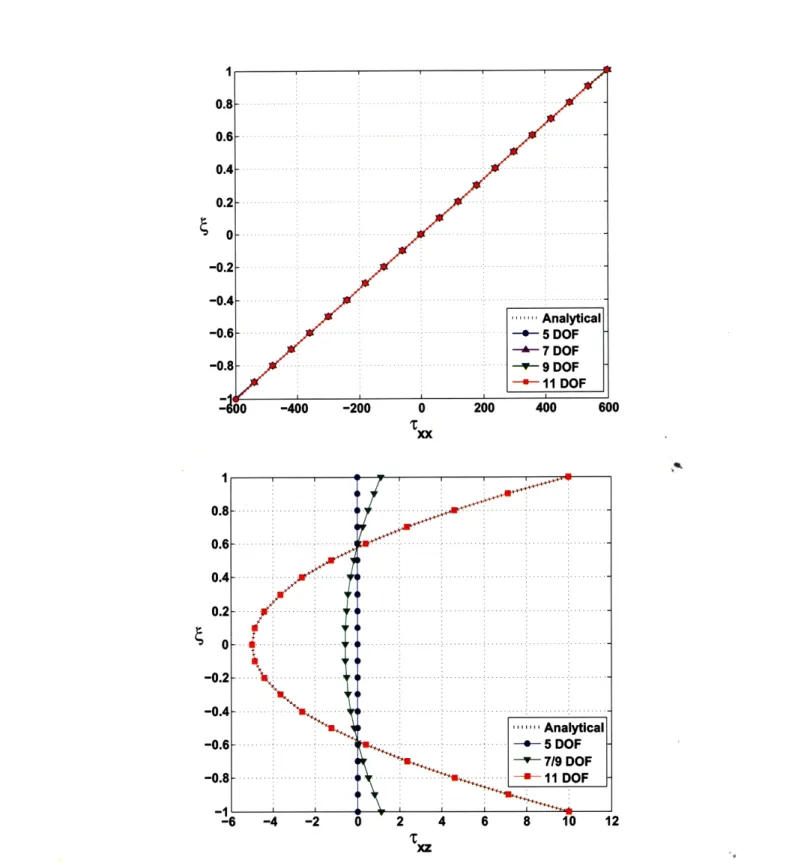
In the first load case, the resultant axial force and shear force are zero but the bending moment is nonzero. As shown in Fig. 1-3, all shell element solutions give the same correct axial stress distribution. However, only the 11-DOF shell element predicts the correct shear stress distribution satisfying the zero resultant shear force condition and the traction boundary conditions on the top and bottom surfaces, TxzJl=-1 = q. In the second load case, the resultant shear force and bending moment are zero, but the axial force is nonzero. Fig. 1-4 shows the calculated stress distri-butions. In this case, both, the 9-DOF shell element and the 11-DOF shell element give the analytical solutions because the cubic displacement function has no effect on the finite element solution. In the third load case, the resultant axial force and bending moment are nonzero, but the resultant shear force is zero. Fig. 1-5 gives the calculated results. The predicted transverse shear stress is quite different using

Table 1.3: Cases of applied traction test

tractions and analytic stress distributions for the in-plane

Case 1 Case 2 Case 3

z z z Tangential 11 Al A -forces on top -. -- t -. q- t t --- _ -~-- t and bottom x _ _-~- x X - --- -.-- --- x and bottom surfaces L L L z z z Equivalent force and - m=qt ____-- _2q _ q moment on -I -l- -- . - -- x mid-surface L L L z z z Analytical tl2 t12 t/2 distribution -3q(L/t) -q(Lt)

of x through ,3q(ut) '" q(Lvt) "7 2q(Ut) the thickness at x = L/2 -t2 -t/2 -t2 z z z Analytical t/2 Vt2 t12V distribution i -q V I of xz through -q12 :q q -q13 q the thickness -t/2

§

using 41 elements along the beam with L = 20.0, t = 1.0, q = 10.0, E = 1.0 x 105,

the various element assumptions. Only the 11-DOF shell element gives an accurate solution satisfying the traction boundary conditions on the top and bottom surfaces,

Txz =1 = q and Txzj =-1 = 0. This result must be expected, since the case is a linear

superposition of cases 1 and 2.

Here, in general, the 11-DOF shell element with the quadratic distribution of the transverse shear stress through its thickness must be used to accurately capture the effect of tangential tractions on the top and bottom shell surfaces (satisfying the traction boundary conditions).

1.3.2

Pressurized cylinder

We consider the pressurized cylinder problem shown in Fig. 1-6. We use this problem to test the predictive capabilities of our shell element in the analysis of a thick-walled structure. A one element model is used, see Fig. 1-6(b). Note that, since the cylinder can only expand or contract in the radial direction due to symmetry, the degrees of freedom for the in-plane quadratic and cubic displacement functions (qi, q2, C1 and

c2) have no effect in the solution of this problem, i.e. the 9-DOF and 11-DOF shell elements will give the same result as the 7-DOF element.

The analytical solutions of this plane strain problem (ezz = 0) for the radial displacement ur, and the radial and circumferential stress Trr and Too are

PR~- PoR0 R R R (P -P) 1 U, = x r + x - (1.22a) 2(A + G)(R - R) x 2G(R - R r (1.2 Pi R - Po R RR(Pi - P) 1 R0 R? Ro - Ri 2 SPRt - P R R R R P -P ₀) 1 TO0+ _R 2_{- R R - Ri} 0 X -_T2 (1.22c)

where Ro and Ri are the outer and inner radii, respectively, P and Pi are the applied pressures, A and G are the Lame constants, and Ri<r<Ro.

Table 1.4 lists the predicted radial displacement of the cylinder mid-surface, and shows that the displacement obtained using the 7-DOF shell element is in good agree-ment with the analytical solution, even when the cylinder is rather thick. However,

xx

-6 -4 -2 0 2 4 6 8 10 12

-r

xz

Figure 1-3: Stress distributions in a cantilever beam under in-plane tractions (Case 1)

0.8-0.6 0.4 0.2 -0.2 -0.4 -0.6- -0.8-150 200 xx 250 300 xz Figure 1-4: Stress distributions

2)

in a cantilever beam under in-plane tractions (Case

. .. .. . . . . . .. .. . ..... . . ...... ... ...... .... ... .. Analytical -05 DOF -- 7 DOF -Y--9 DOF --- I DOF

0.6 0.4 0.2 -0.2 -0.4 -0.6 -0.8 -100 0 100 200 300 400 xt xx xz xz

Figure 1-5: Stress distributions in a cantilever beam under in-plane tractions (Case 3) Analytical -- 5 DOF 7 DOF 9 DOF -- 11 DOF i -1,

\ " P0 x - ...- - -2 R=O.5(Ri+Ro) r (a) (b)

Figure 1-6: Pressurized cylinder in plane strain condition; 0 = 2 °, Pi = 20t, Po = 80t, R = 10.0, E = 1.0 x 104; (a) the whole model, (b) single element representation (only radial displacement is allowed)

in the (almost) incompressible case, the 7-DOF shell element needs to be used with the proposed assumed pressure field. Of course, if the cylinder is thin, both, the 5-DOF and 7-DOF shell elements give virtually the same result for the mid-surface displacement. Figs. 1-7 and 1-8 show the predicted radial and hoop stresses for the thin and thick cases.

Table 1.4: Normalized radial displacement of the pressurized cylinder at r = R

v=0.3 v=0.499999 Shell model 5 DOF 7/9/11 DOF 5 DOF 7/9/11 DOF 7/9/11 DOF (u/p) t = 0.1 0.9962 0.9998 0.9915 0.9998 0.9998 t = 1.0 0.9643 0.9998 0.9203 0.6150 0.9998 t = 2.0 0.9294 0.9998 0.8472 0.0905 0.9998 t = 5.0 0.8234 0.9980 0.6495 0.0025 0.9987

-8 -7 -6 -5 -4 rr 0 0 ee -3 -2 -1 0 1 599

Figure 1-7: Stress distributions in the pressurized cylinder (t = 0.1, Pi = 2.0, Po = 8.0) SAnalytical - 5 DOF - 7/9111 DOF

_..

_...

_.

_r.

_...

_...

_...

..

.

.

.

.

.

.

.

.

.

.

...

/.

.,

...

...

...

rr

440 460 480 500 520 540 -560-- 580

(oe

300 30' - -,1 -':1 - .~---(--- / - - --/ V --- -- -- -- -- -- --- - - - ---L=10 L=10 (a) (b)

Figure 1-9: Single element test for ill-conditioning; (a) director vectors are normal to the mid-surface, (b) director vectors are rotated 30 from the normal direction

1.3.3

Test cases for conditioning of the stiffness matrix

In these problem solutions, we study the conditioning of the stiffness matrices when the thickness of the shell decreases and the material becomes incompressible. The degree of ill-conditioning can be measured by the condition number defined as [6],

cond(K) = max (1.23)

Amin

where Amax and Amin are the maximum and minimum eigenvalues of the stiffness matrix K with rigid body modes excluded. For comparison purposes, we use CK

CK = 10gl0 {cond(K)} (1.24)

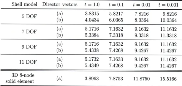
First, a single element with two different orientations of director vectors as shown in Fig. 1-9 is tested. The results are listed in Table 1.5. We see that the condition number of the 3D-shell element with more than five degrees of freedom is for the thin case only about an order of magnitude larger than for the MITC4 shell element with five degrees of freedom. This increase in the condition number is small when

compared to the increase for the 3D-solid element. Note that cond(K)_O(t- 2) for all shell elements while cond(K)-O(t- 4_{) for the 3D-solid element with the thickness,}

t. When the director vectors are not normal to the shell mid-surface as shown in

1010 108 CK =7.4268 0 10 CK =7.1633 il 104-102

-- 9- director vectors are normal to the mid-surface

- director vectors are rotated 300 from the normal direction

10 I I

0 5 10 15 20 25 30 35 40

Mode number

Figure 1-10: Eigenvalues of single element (11-DOF, E = 1.0 x 107, v = 0.3, t = 0.1)

Table 1.5: CK with different element thicknesses, see Fig. 1-9 (E = 1.0 x 107, V = 0.3) Shell model Director vectors t = 1.0 t = 0.1 t = 0.01 t = 0.001

5 DOF (a) 3.8315 5.8217 7.8216 9.8216 (b) 4.0434 6.0365 8.0364 10.0364 7 DOF (a) 5.1716 7.1632 9.1632 11.1632 (b) 5.3384 7.3318 9.3318 11.3318 9 DOF (a) 5.1716 7.1632 9.1632 11.1632 (b) 5.4338 7.4268 9.4267 11.4267 11 DOF (a) 5.1732 7.1633 9.1632 11.1632 (b) 5.4349 7.4268 9.4267 11.4267 3D 8-node

solid element (a) 3.8963 7.8753 11.8750 15.5166

(a) director vectors are normal 30 from the normal direction

108 10-> 10 E = 2.0x108 v 0.3 -e- 5 DOF : CK =6.6487 10---- _{7 DOF : CK} = 6.8473 -F 9 DOF : CK =6.8473 a -u--11 DOF: CK =6.8473 0 200 400 600 800 Mode number

Figure 1-11: Eigenvalues and condition numbers (director vectors are normal to the mid-surface)

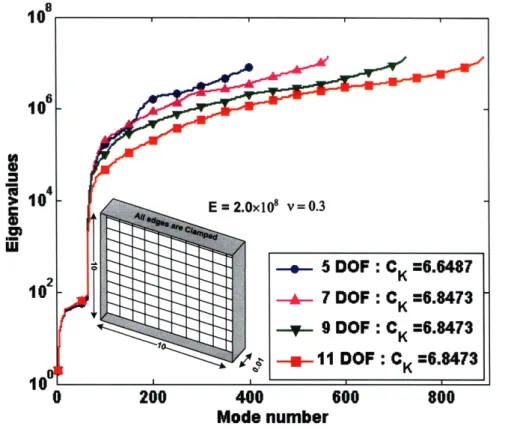
Next, we consider a plate modeled with a 10 x 10 element mesh, see Fig. 1-11, and solve for the eigenvalues and condition numbers, see Ref. [20] for a similar example. We see that the condition numbers of our shell element with 7 to 11 degrees of freedom are only slightly larger than for the MITC4 element. Therefore, in the analysis of shell structures in which 3D effects shall be predicted, the element proposed here is much more reliable than the 3D-solid element.

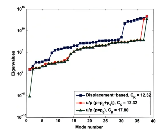
Finally, the single element with an almost incompressible material is considered. In this case, we have inevitably an ill-conditioned stiffness matrix because, for 3D type elements, we have at least one very large eigenvalue corresponding to the volumetric deformation mode. In Fig. 1-12, the displacement-based (without pressure degrees of freedom) shell element shows eight very large eigenvalues that cause the element to be too stiff and lock, see Tables 1.4, 1.7, and 1.9. If we use the element with the u/p formulation, see the assumed pressure field in Eq. (1.21), only two very

1015 1010 10 100 10 -I -Displacement-based, CK = 12.32 -- u/p (p=po+pl4), CK = 12.32 - u/p (p=po), CK = 17.80 i i i i 0 5 10 15 20 25 30 35 40 Mode number

Figure 1-12: Eigenvalues of single element in almost incompressible case (11-DOF,

E = 1.0 x 107, v = 0.499999, t = 0.1); director vectors are normal to the mid-surface

large eigenvalues which correspond to the volumetric expansion mode (the constant pressure mode) and a bending mode (the linear pressure mode through the thickness) are observed. It appears natural to therefore try to use only the constant pressure field (p = P0o) in the u/p formulation, but then the element has a spurious zero energy mode corresponding to the bending mode. Hence, the pressure assumption in Eq. (1.21) is more appropriate.

1.3.4

Hyperboloid shell problems

These shell problems were proposed and studied by Chapelle and Bathe [2, 35, 36] and provide excellent test problems for shell elements. We solve the problems here to investigate the performance of our shell discretizations in the almost incompressible

case.

I I I I

Figure 1-13: The hyperboloid shell problem (E = 2.0 x 1011, t = 0_.0 1_{, po = 1.0 x 106)}

The geometry of the shell mid-surface is given by (see Fig. 1-13) 2 _{+z2= 1 +y} 2_{, y E [-1, 1]}

(1.25)

The hyperboloid mid-surface is subjected to the smoothly varying periodic pressure

p(G) = Po cos(20) (1.26)

If the shell is clamped on both ends, the problem is a membrane-dominated problem, and if the shell is free on both ends, the problem is a bending-dominated problem. We use a 16 x 16 uniform mesh of elements to solve the two problems.

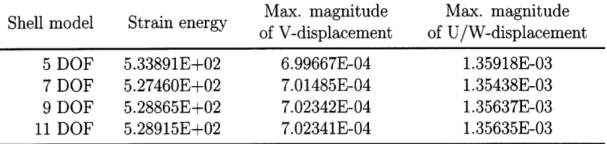
Some results are listed in Tables 1.6, 1.7, 1.8 and 1.9. When the material is compressible (see Tables 1.6 and 1.8), each shell model gives similar results in both the membrane and bending dominated cases. However, when the material is nearly incompressible (see Tables 1.7 and 1.9), the shell elements based on the full three-dimensional constitutive law experience volumetric locking while the 5-DOF MITC4 shell element of course does not lock. Note that, by using the u/p formulation, the volumetric locking of the shell elements using the three dimensional constitutive law

Table 1.6: The clamped-clamped hyperboloid shell (v = 0.333333)

Max. magnitude Max. magnitude

of V-displacement of U/W-displacement

5 DOF 5.33891E+02 6.99667E-04 1.35918E-03

7 DOF 5.27460E+02 7.01485E-04 1.35438E-03

9 DOF 5.28865E+02 7.02342E-04 1.35637E-03

11 DOF 5.28915E+02 7.02341E-04 1.35635E-03

Table 1.7: The clamped-clamped hyperboloid shell (v = 0.499999)

Max. magnitude Max. magnitude

of V-displacement of U/W-displacement

5 DOF 5.70978E+02 7.56065E-04 1.46331E-03

7 DOF 0.40085E+02 0.34764E-04 0.18041E-03

9 DOF 0.74792E+02 0.57580E-04 0.34114E-03

11 DOF 1.18613E+02 1.38555E-04 0.36024E-03

7 DOF (u/p) 5.55900E+02 7.59076E-04 1.45204E-03

9 DOF (u/p) 5.58361E+02 7.60885E-04 1.45701E-03

11 DOF (u/p) 5.58467E+02 7.60881E-04 1.45706E-03

Table 1.8: The free-free hyperboloid shell (v = 0.333333)

Max. magnitude Max. magnitude

of V-displacement of U/W-displacement

5 DOF 4.53983E+05 1.04082E+00 2.10145E+00

7 DOF 4.53820E+05 1.04044E+00 2.10070E+00

9 DOF 4.55217E+05 1.04372E+00 2.10719E+00

11 DOF 4.55237E+05 1.04377E+00 2.10728E+00

Table 1.9: The free-free hyperboloid shell (v = 0.499999)

Max. magnitude Max. magnitude

of V-displacement of U/W-displacement

5 DOF 3.81804E+05 0.87391E+00 1.76575E+00

7 DOF 0.02886E+05 0.00198E+00 0.00846E+00

9 DOF 1.45692E+05 0.33107E+00 0.66385E+00

11 DOF 1.79671E+05 0.40899E+00 0.82209E+00

7 DOF (u/p) 3.81421E+05 0.87293E+00 1.76395E+00

9 DOF (u/p) 3.82368E+05 0.87517E+00 1.76836E+00

(a) (b)

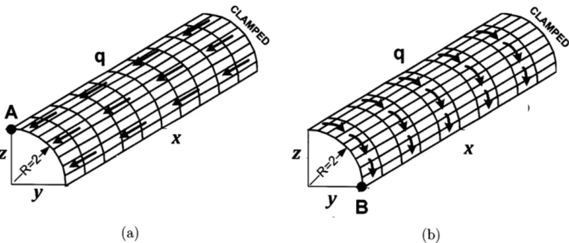
Figure 1-14: The quadrant of a cantilevered cylinder under in-plane tractions (E = 1.0 x 104, v = 0.3, length=40, thickness=0.1); (a) case of applied

longitu-dinal traction (q = 0.1), (b) case of applied circumferential traction (q = 0.007)

1.3.5

A quadrant of a cantilevered cylinder under in-plane

tangential tractions

A quadrant of a cantilevered cylinder under in-plane tangential tractions is tested. The tractions are applied in the longitudinal direction for one case and the circumfer-ential direction for the other case as depicted in Fig. 1-14. In order to see how the load positions affect the solutions, the deformation-dependent tractions are applied on the top, middle and bottom surfaces for each case. Geometrically nonlinear analyses are performed using the 11-DOF shell element with a 10 x 9 mesh of elements in the total Lagrangian framework [6]. The deformed shapes and the displacements and effective stresses are given in Figs. 1-15-1-20. We can see that significant response differences arise depending on how the tractions are applied.

Note that we may obtain very similar results with the 5-DOF MITC4 shell element by applying the resultant forces and moments on the shell mid-surface, especially for a very thin structure as in this problem. Here the effect of the quadratic and cubic in-plane displacements is small enough to be neglected. However, our 11-DOF shell element provides a direct and natural way to include the effects of surface tractions when these are initially unknown (e.g. imposed in a metal forming problem), vary over the shell top and bottom surfaces and the shell thickness changes significantly.

traction applied on bottom surface traction applied on middle surface 40 -1 0 1 2 3 Y Figure 1-15: direction 0 Lu

The deformed shapes when the traction is applied in the longitudinal

2 -*-traction applied on top surface I traction applied on bottom surface

A- traction applied on middle surface

-2 -1.5 -1 -0.5 0 0.5 1 1.5 W (displacement in Z-axis)

Figure 1-16: Displacement in z-direction of point A in Fig. 1-14(a) traction applied

on top surface

-30

0

0 5 10 15 20 25 30 35 Effective Stress on the top surface (Case a)

traction applied on middle surface

Figure 1-17: Fig. 1-14

traction a lied on bottom surface

15

0 5 10 15 20 25 30 35 40

x

Effective Stress on the bottrom surface (Case a)