HAL Id: hal-00875487
https://hal.inria.fr/hal-00875487
Preprint submitted on 22 Oct 2013
HAL is a multi-disciplinary open access
archive for the deposit and dissemination of
sci-entific research documents, whether they are
pub-lished or not. The documents may come from
teaching and research institutions in France or
abroad, or from public or private research centers.
L’archive ouverte pluridisciplinaire HAL, est
destinée au dépôt et à la diffusion de documents
scientifiques de niveau recherche, publiés ou non,
émanant des établissements d’enseignement et de
recherche français ou étrangers, des laboratoires
publics ou privés.
What Makes Affinity-Based Schedulers So Efficient ?
Olivier Beaumont, Loris Marchal
To cite this version:
Olivier Beaumont, Loris Marchal. What Makes Affinity-Based Schedulers So Efficient ?. 2013.
�hal-00875487�
What Makes Affinity-Based Schedulers So Efficient ?
Olivier Beaumont
Loris Marchal
INRIA, LaBRI and Univ. of Bordeaux CNRS, INRIA and ENS Lyon
October 21, 2013
Abstract
The tremendous increase in the size and heterogeneity of supercomputers makes it very difficult to predict the performance of a scheduling algorithm. Therefore, dynamic solutions, where scheduling decisions are made at runtime have overpassed static allocation strategies. The simplicity and efficiency of dynamic schedulers such as Hadoop are a key of the success of the MapReduce framework. Dynamic schedulers such as StarPU, PaRSEC or StarSs are also developed for more constrained computations, e.g. task graphs coming from linear algebra. To make their decisions, these runtime systems make use of some static information, such as the distance of tasks to the critical path or the affinity between tasks and computing resources (CPU, GPU,. . . ) and of dynamic information, such as where input data are actually located. In this paper, we concentrate on two elementary linear algebra kernels, namely the outer product and the matrix multiplication. For each problem, we propose several dynamic strategies that can be used at runtime and we provide an analytic study of their theoretical performance. We prove that the theoretical analysis provides very good estimate of the amount of communications induced by a dynamic strategy, thus enabling to choose among them for a given problem and architecture.
Keywords: Dynamic scheduling, data-aware algorithms, randomized algorithms, performance evalua-tion, linear algebra.
1
Introduction
Recently, there has been a very important change in both parallel platforms and parallel applications. On the one hand, computing platforms, either clouds or supercomputers involve more and more computing resources. This scale change poses many problems, mostly related to unpredictability and failures. First, the size of the platform is expected to decrease the MTBF (Mean Time Between Failures) and is likely to make fault tolerance issues unavoidable. On the other hand, the use of runtime fault tolerance strategies that would be agnostic to the application, such as those based on checkpointing [1, 2, 3] or replication [4, 5], are expected to induce a very large and maybe prohibitive overhead. Moreover, due to the size of the platforms, their complex network topologies, the use of heterogeneous resources, NUMA effects, the number of concurrent simultaneous computations and communications, it is impossible to predict exactly the time that a specific task will take. Unpredictability makes it impossible to statically allocate the tasks of a DAG onto the processing resources and dynamic strategies are needed. In recent years, there has been a large amount of work in this direction, such as StarPU [6], DAGuE and PaRSEC [7, 8] or StarSs [9]. The main characteristics of these schedulers is that they make their decisions at runtime, based on the expected duration of the tasks on the different kind of processing units (CPUs, GPUs,...) and on the expected availability time of the task input data, given their actual location. Thanks to these information, the scheduler allocates the task to the resource that will finish its processing earlier. Moreover, all these runtime systems also make use of some static information that can be computed from the task graph itself, in order to decide the priority between several ready tasks. This information mostly deals with the estimated critical path as proposed in HEFT [10] for instance.
On the other hand, there has been a dramatic simplification of the application model in many cases, as asserted by the success of MapReduce [11, 12, 13] or Divisible Load [14, 15, 16, 17, 18]. These models, due to their simplicity, make fault tolerance and unpredictability issues less critical, since it is possible, when reaching the end of the execution to re-launch late tasks. Therefore, as noted in [19], those paradigms are widely used even for non linear complexity tasks. On the other hand, executing non linear complexity tasks on such platforms makes it necessary to replicate data and therefore, minimizing the overall volume of communications becomes a non trivial issue.
Our goal in this paper is to provide a sound theoretical basis for the analysis of the performance of runtime schedulers. Thus, we will concentrate on two elementary kernels, namely the outer product and the matrix multiplication. In both cases, as described in [19], input vectors or input matrices need to be replicated and basic dynamic strategies that allocate tasks at random to processors fail to achieve reasonable communication volumes with respect to known lower bounds. In the present paper, our contribution is twofold. First, we propose for both the outer product and the matrix multiplication a set of dynamic runtime random strategies that take into account the actual placement of replicated data to assign tasks to processing resources. We prove using extensive simulations for a large set of distribution of heterogeneous resources that these runtime strategies are efficient in practice and induce a communication volume that is close to the lower bound. Our second and most original contribution is to propose to analyze the communication volume as a dynamic process that can be modeled by an Ordinary Differential Equation (ODE). We prove that the analytic communication volume of the solution of the ODE is close to the actual communication volume as measured using simulations. We also prove that the analysis of the solution of the ODE can be used in order to tune some parameters of the runtime schedulers (for instance, when to switch from one strategy to another). This simple example attests the practical interest of the theoretical analysis of dynamic schedulers, since it shows that the analytic solution can be used in order to incorporate static knowledge into the scheduler.
A very successful example of dynamic schedulers lies in MapReduce implementations. The MapReduce framework [12] which has been popularized by Google, has recently received at lot of attention. It allows users without particular knowledge in parallel algorithm to harness the power of large parallel machines. In MapReduce, a large computation is broken into small tasks that run in parallel on multiple machines, and scales easily to very large clusters of inexpensive commodity computers. Hadoop [20] is the most popular open-source implementation of the MapReduce framework, originally developed by Yahoo! to manage jobs that produce hundreds of terabytes of data on thousands of cores. Examples of applications implemented with Hadoop can be found at http://wiki.apache.org/hadoop/PoweredBy. A crucial feature of MapReduce is its inherent capability of handling hardware failures and processing capabilities heterogeneity, thus hiding this complexity to the programmer, by relying on on-demand allocations and a detection of nodes that perform poorly (in order to re-assign tasks that slow down the process).
In Hadoop, load balancing is achieved through the distribution of data on the computing nodes. Hadoop’s Distributed File System (HDFS) splits input files into even-sized fragments, and distributes the fragments to pool of computing nodes [21]. Each fragment is replicated both for fault-tolerance and for faster data access. By default, HDFS replicates each fragment on three nodes (two of these nodes are on the same rack to avoid high bandwidth utilization when updating files). Hadoop’s load balancing strategy assumes a homogeneous computing environment, and is not optimal in heterogeneous and dynamic environments (such as virtualized clusters). Several strategies have been proposed to overcome these shortcomings, by better estimating task progress [13] or distributing data fragments according to the estimated processor computing speed [22].
In this paper, we propose a few dynamic randomized strategies to deal with more complicated, although very regular data access patterns. The outline of the paper is as follows. In Section 2, we consider the problem of computing the outer product of two vectors. We first present a basic randomized runtime strategy that allocates tasks to processing resources so as to reuse data at much as possible.. We also propose an analytical model of this algorithm in Section 2.3, that suggests an improvement of the randomized strategy whose efficiency is demonstrated through simulations in Section 2.4. We also propose more sophisticated randomized algorithms, that performs better at the price of an increase in the complexity of scheduling and resource allocation decisions in Section 2.5. Section 3 follows the same outline with matrix multiplication. Concluding remarks and perspectives are given in Section 4.
2
Randomized dynamic strategies for the outer-product
2.1
Notations
We consider the problem of computing the outer-product abt of two large vectors a and b of size N , i.e. to
compute all values ai× bj, ∀1 ≤ i, j ≤ N . The computing domain can therefore be seen as a matrix. For
granularity reasons, we will consider that a and b are in fact split into N/l blocks of size l and that a basic operation consists in computing the outer product of two (small) vectors of size l.
As stated above, we target heterogeneous platforms consisting of p processors P1, . . . , Pp, where the speed
of processor Pi, i.e. the number of outer product of size l vectors that Pi can do in one time unit, is given
by si. Note that the randomized strategies that we propose are agnostic to processor speeds, but they are
demand driven, so that a processor with a twice larger speed will request work twice faster.
We will assume throughout the analysis that it is possible to overlap computations and communications. This can be achieved with dynamic strategies by uploading a few blocks in advance at the beginning of the computations and then to request work as soon as the number of blocks to be processed becomes smaller than a given threshold. Determining this threshold would require to introduce a communication model and a topology, what is out of the scope of this paper, and we will assume that the threshold is known. In practice, the number of tasks has been observed to be small in [23, 24] even though a rigorous algorithm to estimate it is still missing.
As we observed [19], performing a non linear complexity task as a Divisible Load or as a MapReduce operation requires to replicate initial data. Our objective is to minimize the overall amount of communica-tions, i.e. the total amount of data (the number of blocks of a and b) sent by the master initially holding the data (or equivalently by the set of devices holding the data since we are interested in the overall volume only), under the constraint that a perfect load-balancing should be achieved among resources allocated to the outer product computation. Indeed, due to data dependencies, if we were to minimize communications without this load-balancing constraint, the optimal (but very inefficient) solution would consist in making use of a single computing resource so that each data block would be sent exactly once.
2.2
Basic dynamic randomized strategies
As mentioned above, vectors a and b are split into N/l data blocks. In the following, we denote by ai the
ith block of a (rather than the ith element of a) since we always consider elements by blocks. As soon as a processor has received two data blocks ai and bj, it can compute the block Mi,j = (abt)i,j = aibtj. This
elementary task is denoted by Ti,j. All data blocks are initially available at the master node only.
One of the simplest strategy to allocate computational tasks to processors is to distribute tasks at random: whenever a processor is ready, a task Ti,j is chosen uniformly at random among all available tasks
and is allocated to the processor. If the data corresponding to this task, that is data blocks ai and bj, are
not available on the processor, they are sent by the master to the processor. We denote this strategy by RandomOuter. Another simple option is to allocate tasks in lexicographical order of indices (i, j) rather than randomly. This strategy will be denoted as SortedOuter.
Both previous algorithms are expected to induce a large amount of communications because of data replication. Indeed, in these algorithms, there is no reason why the data sent for the processing of tasks on a given processor Pk may be used for upcoming tasks. It would be much more beneficial, when receiving a
new pair of blocks (ai, bj), to compute all possible products aibtj0 and ai0btj for all data blocks ai0 and bj0 that
are already on Pk. This is the intuition of strategy BasicOuter: whenever a processor asks for a new task,
it receives two new blocks ai and bj and performs all possible tasks with these new blocks. This strategy is
described on Algorithm 1.
2.3
Theoretical analysis of BasicOuter strategy
In this section, our aim is to provide an analytical model for Algorithm BasicOuter. Analyzing such a strategy is crucial in order to assess the efficiency of runtime dynamic strategies and in order to tune the
Algorithm 1: BasicOuter strategy. while there are unprocessed tasks do
Wait for a processor Pk to finish its tasks
I ← {i such that Pk owns ai}
J ← {j such that Pk owns bj}
Choose i /∈ I and j /∈ J uniformly at random Send ai and bj to Pk
Allocate all tasks of {Ti,j} ∪ {Ti,j0, j0∈ J } ∪ {Ti0,j, i0 ∈ I} that are not yet processed to Pk and
mark them processed
parameters of dynamic strategies or to choose among different strategies depending on input parameters. In what follows, we assume that N , the size of vectors a and b, is large and we consider a continuous dynamic process whose behavior is expected to be close to the one of BasicOuter. In what follows, we concentrate on processor Pk whose speed is sk. At each step, BasicOuter chooses to send one data block
of a and one data block of b, so that Pk knows the same number of data blocks of a and b. As previously,
we denote by M = abtthe result of the outer product and by T
i,j the tasks that corresponds to the product
of data blocks ai and bj
We denote by x = y/N the ratio of elements of a and b that are known by Pk at a given time step
of the process and by tk(x) the corresponding time step. We concentrate on a basic step of BasicOuter
during which the fraction of data blocks of both a and b known by Pk goes from x to x + δx. In fact, since
BasicOuter is a discrete process and the ratio known by Pk goes from x = y/N to x + l/N = y/N + l/N .
Under the assumption that N is large, we assume that we can approximate the randomized discrete process by the continuous process described by the corresponding Ordinary Differential Equation on expected values. The proof of convergence is out of the scope of this paper but we will show that this assumption is reasonable through simulation results in Section 2.5. The use of mean field techniques for analyzing such dynamic processes has been advocated in [25, 26] but a rigorous proof is left for future work.
In what follows, we denote by gk(x) the fraction of tasks Ti,j that have not been computed yet. Let us
remark that during the execution of BasicOuter, tasks Ti,j are greedily computed as soon as a processor
knows the corresponding data blocks of aiand bj. Therefore, at time tk(x), all tasks Ti,jsuch that Pk knows
data blocks ai and bj have been processed and there are x2N2/l2 such tasks. Note also that those tasks
may have been processed either by Pk or by another processor Plsince processors compete to process tasks.
Indeed, since data blocks of a and b are possibly replicated by BasicOuter on several processors, then both Pk and Pl may know at some point ai and bj. In practice, this is the processor that learns both ai and bj
first that will compute Mi,j.
Based on this remark, we are able to prove the following Lemma Lemma 1. gk(x) = (1 − x2)αk, where αk=
P i6=ksi
sk .
Proof. Let us consider the tasks that have been computed by all processors between tk(x) and tk(x + δx).
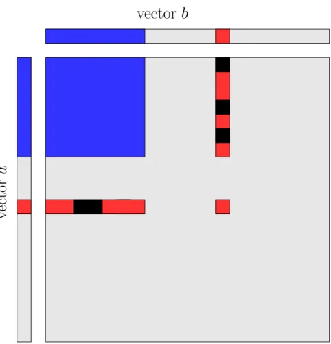
As depicted on Figure 1, these tasks can be split into two sets
• The first set of tasks consists in those that can be newly processed by Pk between tk(x) and tk(x + δx).
Pk has the possibility to combine the δx new elements of a with the x already known elements of b
(and to combine the δx new elements of b with the x already known elements of a). There is therefore a total (at first order) of 2xδx such tasks. Among those, by definition of g, the expected number of tasks that have not already been processed by other processors is given by 2xδxg(x). Therefore, the expected duration is given by 2xδxg(x)s
k .
• The second set of tasks consists in those computed by other processors Pi, i 6= k. Our assumption
v
ector
a
vector b
Figure 1: Illustration for the proof of Lemma 1. The top-left blue rectangle represents the data owned by the processor at time tk(x) (a permutation of the rows and columns has been applied to have it in the upper
left corner). The new elements δx are depicted in red, as well as the corresponding available tasks. Note that some tasks (in black) corresponding to the combination of δx with the known elements have already been processed by other processors.
in advance), so that processors Pi, i 6= k will keep processing tasks between tk(x) and tk(x + δx) and
will process on expectation 2xδxg(x)s
k
P
i6=ksi tasks.
Therefore, we are able to estimate how many tasks will be processed between tk(x) and tk(x + δx) and
therefore to compute the evolution (on expectation) of gk. More specifically, we have
gk(x + δx) × (1 − (x + δx)2)x = gk(x) × (1 − x2) − 2xδxg(x) − 2xδxg(x)P i6=ksi sk ,
what gives at first order
gk(x + δx) − gk(x) = gk(x)δx −2xαk 1 − x2, where αk= P i6=ksi sk .
Therefore, the evolution of gk with x is given by the following ordinary differential equation
g0k(x) gk(x)
= −2xαk 1 − x2
where both left and right terms are of the form f0/f , what leads to
ln(gk(x)) = αkln(1 − x2) + K
and finally to
gk(x) = exp(K) ln(1 − x2)αk,
where exp(K) = 1 since gk(0) = 1. This achieves the proof of Lemma 1.
Remember that tk(x) denotes the time necessary for Pk to know x elements of a and b. Then,
Lemma 2. tk(x)(Pisi) = 1 − (1 − x2)αk+1.
Proof. We have seen that some of the tasks that could have been processed by Pk (tasks Ti,j such that Pk
knows both ai and bj) have indeed been processed by other processors. In order to prove the lemma, let us
denote by hk(x) the number of such tasks at time tk(x + δx). Then
hk(x + δx) = hk(x) + 2xδx(1 − gk(x))
by definition of gk so that, using Lemma 1,
h0k(x) = 2x − 2x(1 − x2)αk and hk(x) = x2+ (1 − x2)αk+1 αk+ 1 + K and since hk(0) = 0, hk(x) = x2+ (1 − x2)αk+1 αk+ 1 − 1 αk+ 1 .
Moreover, at time tk(x), all the tasks that could have been processed by Pk have
• either been processed by Pk and there are exactly tk(x)sk such elements since Pk has been processing
• or processed by other processors and there are exactly hk(x) such tasks by definition of hk. Therefore, x2= hk(x) + tk(x)sk and finally tk(x) X i si = 1 − (1 − x2)αk+1,
which achieves the proof of Lemma 2.
Above equations well describe the dynamics of BasicOuter as long as it is possible to find blocks of a and b that enable to compute enough unprocessed tasks. On the other hand, at the end, it is better to switch to another algorithm, where random unprocessed tasks Ti,j are picked up randomly, which possibly
requires to send both blocks ai and bj. In order to decide when to switch from one strategy to the other, we
introduce an additional parameter β.
As noted in [19], a lower bound on the communication volume received by Pk (if perfect load balancing
is achieved) is given by 2Npsk/Pisi. Indeed, in a very optimistic setting, each processor is dedicated to
computing a “square” area of M = abt whose area is proportional to its relative speed. In this situation, the amount of communication for Pk is the half perimeter of this square of area N2Psk
isi. We will switch
from the BasicOuter to the RandomOuter strategy when the fraction of elements received by Pk is
N2× (2pβs
k/Pisi), and the problem becomes to choose the value of β.
Lemma 3. Pk receives 2pβsk/Pisi at time
(1−e−β) P
isi
(at first order when the number of processors becomes large).
Proof. Since tk(x)Pisi = 1 − (1 − x2)αk+1, when x =pβsk/Pisi, then
tk(x) X i si = 1 − e P isi sk ln(1 − βPsk isi )
= 1 − e−β (at first order,) which achieves the proof of Lemma 3.
One remarkable characteristics of above result is that it does not depend on k anymore. Otherwise stated, at time T =P
isi(1 − eβ), each processor Pi, ∀i has received
√
β times more than the lower bound. The following lemma provides the overall communication volume if one switches between the two strate-gies for parameter β.
Lemma 4. The ratio between the overall volume of communications and the lower bound if the switch between both strategies is made for parameter β is given by
p β + e −βN lP k q sk P isi ,
where l is the size of a block.
Proof. When the switch between strategies occurs, processor Pk has received 2
√ βq sk
P
isi so that the overall
volume of communication isP k2 √ βq sk P isi, i.e. √
β times the lower bound P
k2
q s
k P
isi. Moreover, when
the switch occurs, there remains a fraction e−β of tasks to be done, i.e. e−β ×Nl22 tasks. Since data needed
The above formula is not trivial to solve analytically, but finding the value of β that minimizes the ratio can be done numerically by solving the following equation:
1 2√β = e−βN lP k q s k P isi .
2.4
Towards better dynamic strategies
Before presenting the result of the simulations assessing the accuracy of the previous analysis, we present a few more dynamic runtime strategies which aim at improving the communication amount of BasicOuter. With the previous strategy, when a processor Pk receives some data block ai and bj, it may be the case
that Pk cannot process any tasks, since all the corresponding tasks are or were already processed by other
processors. This is especially true at the end of the execution. We have explored several ways of transforming BasicOuter to avoid this, and in this paper we present two of them that are both representative and successful.
The first idea is, when sending aiand bj, to check that at least task Ti,j is not processed. In other words,
instead of choosing two data blocks not on Pk, we choose an unprocessed task Ti,j such that ai and bj are
not on Pk. This strategy is denoted by DynUnprocessedOuter. Note that during the execution, the
number of unprocessed tasks Ti,j may vary for different blocks ai (and bj). By picking an unprocessed tasks,
we naturally increase the probability of choosing a block ai (and bj) with a higher density of unprocessed
tasks Ti,j. Thus, in addition to the guarantee that at least of task is available for Pk, we hope that this
strategy will allow to get more available tasks at each step.
The second strategy to avoid downloading useless data blocks on a processor Pk is to select data blocks
ai and bj with a guarantee that Pk will have some task to process, i.e. such that the set of unprocessed
tasks Ti,j0 and Ti0,j (for all ai0 bj0 already on Pk) is not empty. This strategy is called DynUsefulOuter.
Note that both previous strategies are more time-consuming, as they need (i) either to maintain complex data structures with up-to-date information on blocks, or (ii) to recompute the information at runtime when a new processor becomes available.
The last proposed strategy for the outer-product differs from the previous ones, as it allocates a single task at a time to each processor. The idea is to classify all unprocessed tasks in three categories with respect to processor Pk:
• Tasks of cost 0 are tasks Ti,j such that both ai and bi are already on processor Pk.
• Tasks of cost 1 are tasks Ti,j such that only one of ai and bi is available on Pk.
• Tasks of cost 2 are tasks Ti,j such that both ai and bi are not on Pk.
This strategy, called DynBlocksOuter, allocates to each available processor a task of cost 0 in any, or a task of cost 1 if any, and in the lastly a task of cost 2 if no task with smaller cost is available. Similarly to the previous two involved strategies, it is necessary to maintain complex data when allocating tasks.
2.5
Simulation Results
In order to study the accuracy of the previous theoretical analysis, we slightly modify the BasicOuter strategy to better fit with the analysis. As in the analysis, when the number of unprocessed tasks becomes small, we switch to the RandomOuter strategy: unprocessed tasks are sent to the available processors as in the RandomOuter strategy. This mixed strategy is called BasicOuter2. As in the analysis, the change occurs when the number of unprocessed tasks becomes smaller than e−βN2/l2. We discuss in Paragraph 2.5.1 below how to estimate β in a dynamic runtime environment.
We have performed simulations to study the performance of the previous strategies and the accuracy of the theoretical analysis. Processor speeds are chosen uniformly in the interval [10, 100], which means a large degree of heterogeneity. Each point in Figures 2 and 3 is the average over 10 simulations1. The communication amount of each strategy is normalized by the lower bound computed in Section 2.3.
1The standard deviation is always small (at most 0.12 for BasicOuter and smaller than 0.1 for all other strategies) and
Normalized
comm
unication
amoun
t
Number of processors (logarithmic scale)
4000 2000 400 200 DynBlocksOuter DynUnprocessedOuter DynUsefulOuter BasicOuter2 Analysis BasicOuter 2 10000 1000 100 3 1
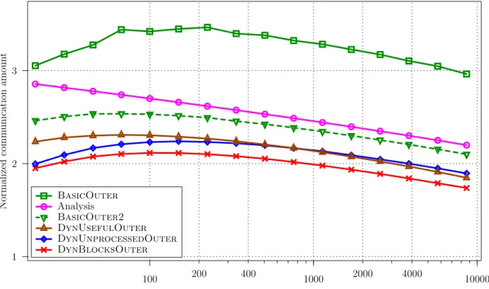
Figure 2: Performance of all outer-product strategies (except RandomOuter and SortedOuter) for vectors of size N/l = 1000 blocks ((N/l)2 tasks).
Matrix size in number of blocks (logarithmic scale) Normalized comm unication amoun t 2000 400 200 40 20 SortedOuter RandomOuter 4 2 1 1000 100 10 3 5
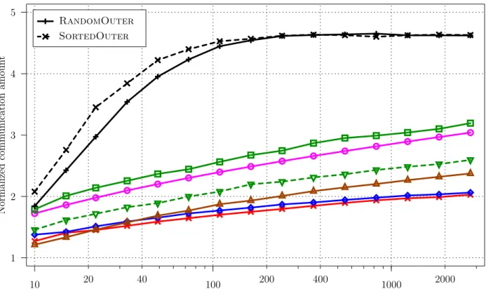
Figure 3: Performance of all outer-product strategies for p = 10 processors. Same legend as Figure 2 for strategies in common.
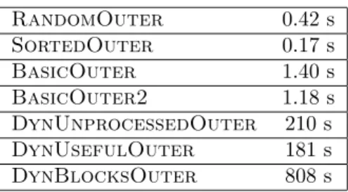
The simulations results show that the simplest strategies (RandomOuter and SortedOuter) are largely outperformed by basic data-aware policies (on Figure 2, their normalized communication amount is around 20 and thus is not depicted). We also notice that the theoretical analysis is close to the BasicOuter2 strategy as expected. The more involved policies described in Section 2.4 allow to reduce even more the amount of communications. The DynBlocksOuter strategy, that allocates blocks one after the other according to their cost, performs extremely well whenever N/l or p is large, with a communication amount almost always smaller than twice the lower bound. These excellent results come at the price of a larger scheduling time, as outlined in Table 1. Note that even if the cumulative scheduling time is large for the best strategies (up to 14 minutes), this may not be a problem for a large computing system including p=1000 processors and (N/l)2= 106 computation tasks.
RandomOuter 0.42 s SortedOuter 0.17 s BasicOuter 1.40 s BasicOuter2 1.18 s DynUnprocessedOuter 210 s DynUsefulOuter 181 s DynBlocksOuter 808 s
Table 1: Running time for N/l = 1000 and p = 1000.
2.5.1 Runtime estimation of β
In order to estimate the β parameter in the BasicOuter2 strategy, it seems necessary to know the processing speed, as β depends onP
kpsk/Pisi. However, we have noticed a very small deviation of β with the speeds.
In particular, for a large range of N/l and p values (namely, p in [10; 1000] and N/l ∈ [max(10,√p), 1000]), for processor speeds in [10, 100], β goes from 1 to 8 but the standard deviations (using 100 tries) is at most 0.018. Our idea is to approximate β with βhom obtained using a homogeneous platform with the same
number of processor and blocks. The relative difference between βhom and the average β of the previous
set is always smaller than 5% (and smaller than 1.1% if N/l > 100√p). Moreover, the relative difference between the approximation ratio on the communication volume predicted using a homogeneous platform and the one obtained using the previous distribution is always smaller than 1%. Thus, it is possible to totally specify the BasicOuter2 strategy and to predict is approximation ratio with very good accuracy while being totally agnostic to processor speeds.
3
Matrix Multiplication
3.1
Notations and Basic Dynamic Random Strategies
We first adapt the notations to the problem of computing the matrix product C = AB. As in the previous section, we consider that all transfers are done with blocks of size l×l, so that all three matrices are composed of N2/l2 blocks and A
i,j denotes the block of A on the ith row and the jth column. The basic computation
step is a task Ti,j,k, which corresponds to the product Ci,j ← Ci,j+ Ai,kBk,j. To perform such a task, a
processor has to receive the input data from A and B (of size 2l2), and to send the result (of size (N/l)2)
back to the master at the end of the computation. Thus, it results in a total amount of communication of 3 (N/l)2. As previously, in order to minimize the amount of communication, our goal is to take advantage
of the blocks of A, B and C already sent to a processor Pu when allocating a new task to Pu. Note that at
the end of the computation, all Ci,j are sent to the master which computes the final results by adding the
different contribution. This computational load is much smaller than computing the products Ti,j,k and is
thus neglected. As in the outer product case, the value of l and therefore the time spent to compute a task must be kept relatively small in order to avoid load-unbalance.
The simple strategies RandomOuter and SortedOuter translates very easily for matrix multipli-cation into strategies RandomMatrix and SortedMatrix. We adapt the BasicOuter strategy into BasicMatrix as follows. We ensure that at each step, for each processor Pu there exists sets of indices I, J
and K such that Pu owns all values Ai,k, Bk,j, Ci,jfor i ∈ I, j ∈ J and k ∈ K, so that it is able to compute
all corresponding tasks Ti,j,k. When a processor becomes idle, instead of sending it a single block of A, B
and C, we choose a new tuple (i, j, k) (with i /∈ I , j /∈ J and k /∈ K) and send to Pu all the data needed to
extend the sets I, J, K with (i, j, k). This corresponds to sending 3(2|I| + 1) data blocks to Pu (see details
in Algorithm 2, and note that |I| = |J | = |K|). Then, all the (yet unprocessed) tasks that can be done with the new data are allocated to Pu.
Algorithm 2: BasicMatrix strategy. while there are unprocessed tasks do
Wait for a processor Pu to finish its task
I ← {i such that Puowns Ai,k for some k}
J ← {i such that Puowns Bk,j for some k}
K ← {i such that Pu owns Ai,k for some i}
Choose i /∈ I , j /∈ J and k /∈ K uniformly at random Send the following data blocks to Pu:
• Ai,k0 for k0 ∈ K ∪ {k} and Ai0,k for
i0∈ I ∪ {i}
• Bk,j0 for j0 ∈ J ∪ {j} and Bk0,j for
k0∈ K ∪ {k}
• Ci,j0 for j0 ∈ J ∪ {j} and Ci0,j for
i0∈ I ∪ {i}
Allocate all tasks {Ti0,j0,k0with i0= i or j0 = j or k0= k} that are not yet processed to Puand
mark them processed
3.2
Theoretical analysis of dynamic randomized strategies
In this section, our aim is to provide an analytical model for Algorithm BasicMatrix as we did for Algorithm BasicOuter in Section 2.3. The analysis of both processes is in fact rather similar, so that we will mostly state the corresponding lemmas, since the proofs are similar to those presented in Section 2.3.
In what follows, we will assume that N , the size of vectors A, B and C, is large and we will consider a continuous dynamic process whose behavior is expected to be close to the one of BasicMatrix. In what follows, as in Section 2.3, we will concentrate on processor Pk whose speed is sk. We will also denote by
C = A × B the result of the outer product. Note that in this Section, Ai,k denotes the element of A on the
ith row and jth column.
Let us assume that there exist 3 index sets I, J and K such that
• Pk knows all elements Ai,k, ∀i ∈ I, ∀k ∈ K,, Bk,j, ∀k ∈ K, ∀j ∈ J and Ci,j, ∀i ∈ I, ∀j ∈ J .
• I, J and K have size y.
In Algorithm BasicMatrix, at each step, Pk chooses to increase its knowledge by increasing y by l
(which requires to receive ly elements of each A, B and C). As we did in Section 2.3, we will concentrate on x = y/N , and assuming that N is large, we will change the discrete process into a continuous process described by an ordinary differential equation depicting the evolution of expected values and we will rely on extensive simulations to assert that this approximation is valid (rather than proving it using mean field techniques as done in [25, 26]).
In this context, let us consider that an elementary task T (i, j, k) consists in computing Ci,j+ = Ai,kBk,j.
There are N3 such tasks. In what follows, we will denote by gk(x) the fraction of elementary tasks that
have not been computed yet. The following lemma enable to understand the dynamics of gk (all proofs are
omitted because they are very similar to those of Section 2.3). Lemma 5. gk(x) = (1 − x3)αk, where αk=
P i6=ksi
sk .
Let us now denote by tk(x) the time step such that index sets I, J and K have size x. Then,
Lemma 6. tk(x)Pisi = 1 − (1 − x3)αk+1.
Above equations well describe the dynamics of BasicMatrix as long as it is possible to find elements of A, B and C that enable to compute enough unprocessed elementary tasks. On the other hand, as in the case of BasicOuter, at the end, it is better to switch to another algorithm, where random unprocessed elementary tasks T (i, j, k) are picked up randomly, what requires possibly to send all values of Ai,k, Bk,j
and Ci,j. In order to decide when to switch from one strategy to the other, let us introduce the additional
parameter β.
As in the outer-product problem, a lower bound on the communication volume received by Pk can be
obtained by considering that each processor has a cube of tasks Ti,j,kto compute, proportional to its relative
speed. The edge-size of this cube is thus N (sk/Pisi) 1/3
. To compute all tasks in this cube, Pk needs to
receive a square of each matrix, that is 3N (sk/Pisi)2/3. We switch between strategies when the number of
elements received by Pk is 3(βsk/Pisi)2/3, and the problem becomes to choose the value of β.
Lemma 7. Pk receives 3(βsk/Pisi)2/3at timePisi(1 − e−β) (at first order when the number of processors
becomes large).
The following lemma provides the overall communication volume if one switches between the two strate-gies for parameter β.
Lemma 8. The ratio between the overall volume of communications generated by BasicMatrix and the lower bound if the switch between both strategies is made for parameter β is given by
p β + e −βN lP k(β sk P isi) 2 3 .
3.3
Better Dynamic Strategy and Simulation Results
As we did for the outer-product strategy, we slightly modify the BasicMatrix strategy to switch to a basic random policy when the number of remaining blocks is smaller than e−β(N/l)3. This policy is denoted by
BasicMatrix2. Similarly, the DynBlocksOuter strategy can easily be adapted for the matrix multipli-cation problem: when looking for a new task to process on Pu, each unprocessed task Ti,j,k is given a cost
which is the number of data blocks among Ai,k, Bk,j, Ci,j which have to be sent to Pu before the task can
be processed. The DynBlocksMatrix strategy first allocate tasks of cost 0, then tasks of cost 1, cost 2 and lastly cost 3.
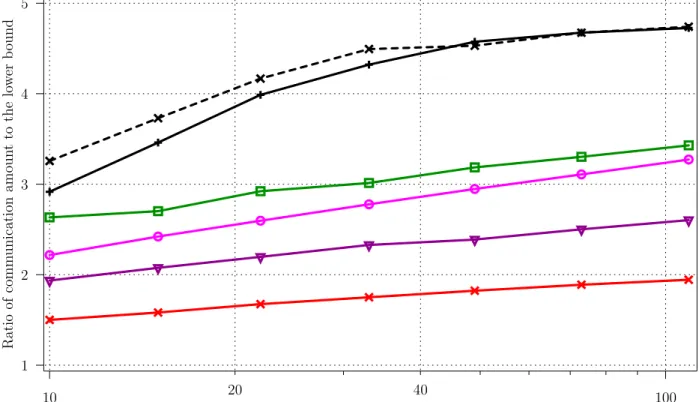
The previous strategies were compared through simulations in the same setting as in Section 2.5. The amount of communication of all strategies are normalized using the lower bound computed in the previous section, and presented in Figure 4 and 5.
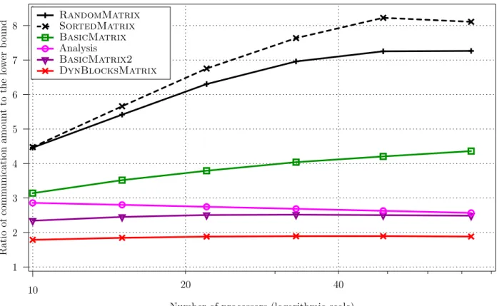
As for the outer-product problem, we notice that data-aware strategies largely outperform simple strate-gies. Similarly, the analysis of BasicMatrix2 is able to accurately predict its performance, and more involved strategies like DynBlocksMatrix are able to drastically reduce the total amount of communica-tion.
40 20 Ratio of comm unication a moun t to the lo w er b ound
Number of processors (logarithmic scale) DynBlocksMatrix BasicMatrix2 Analysis BasicMatrix SortedMatrix RandomMatrix 4 5 6 7 8 10 1 2 3
Matrix size in number of blocks (logarithmic scale) Ratio of comm unication a moun t to the lo w er b ound 40 20 100 4 3 2 10 1 5
4
Conclusion and perspectives
The conclusion of this paper follows two directions. Firstly, we have proposed a set of randomized dynamic scheduling strategies for the outer product and the matrix multiplication. We have proved that affinity-based strategies that aim to place tasks on processors such that the induced communication is as small as possible perform very well. Secondly, for one of the strategies, we have even been able to propose an Ordinary Differential Equation whose solution describes very well the dynamics of the system. Maybe even more important is the proof that the analysis of the solution of the ODE can be use to inject some static knowledge which is useful to increase the efficiency of dynamic strategies. A lot remains to be done in this domain, that we consider as crucial given the practical importance of dynamic runtime schedulers. First, it would be of interest to be able to provide analytical models for all the dynamic schedulers that we have proposed. Then, it would be very useful to extend the analysis to applications involving both data and precedence dependencies. Extending this work to regular dense linear algebra kernels such as LU or QR factorizations is a promising first step in this direction.
References
[1] M. Bougeret, H. Casanova, M. Rabie, Y. Robert, and F. Vivien, “Checkpointing strategies for parallel jobs,” in Proceedings of the International Conference for High Performance Computing, Networking, Storage and Analysis (SuperComputing 2011). IEEE, 2011.
[2] F. Cappello, H. Casanova, and Y. Robert, “Checkpointing vs. migration for post-petascale supercom-puters,” Proceedings of the 39th International Conference on Parallel Processing (ICPP’2010), 2010. [3] A. Bouteiller, F. Cappello, J. Dongarra, A. Guermouche, T. H´erault, and Y. Robert, “Multi-criteria
checkpointing strategies: response-time versus resource utilization,” in Euro-Par 2013 Parallel Process-ing. Springer, 2013, pp. 420–431.
[4] C. Wang, Z. Zhang, X. Ma, S. S. Vazhkudai, and F. Mueller, “Improving the availability of supercom-puter job input data using temporal replication,” Comsupercom-puter Science-Research and Development, vol. 23, no. 3-4, pp. 149–157, 2009.
[5] K. Ferreira, J. Stearley, J. Laros III, R. Oldfield, K. Pedretti, R. Brightwell, R. Riesen, P. Bridges, and D. Arnold, “Evaluating the viability of process replication reliability for exascale systems,” in Proceedings of 2011 International Conference for High Performance Computing, Networking, Storage and Analysis. ACM, 2011, p. 44.
[6] C. Augonnet, S. Thibault, R. Namyst, and P.-A. Wacrenier, “Starpu: a unified platform for task scheduling on heterogeneous multicore architectures,” Concurrency and Computation: Practice and Experience, vol. 23, no. 2, pp. 187–198, 2011.
[7] G. Bosilca, A. Bouteiller, A. Danalis, T. Herault, P. Lemarinier, and J. Dongarra, “DAGuE: A generic distributed dag engine for high performance computing,” Parallel Computing, vol. 38, no. 1, pp. 37–51, 2012.
[8] G. Bosilca, A. Bouteiller, A. Danalis, M. Faverge, T. Herault, and J. J. Dongarra, “PaRSEC: A pro-gramming paradigm exploiting heterogeneity for enhancing scalability,” IEEE Computing in Science and Engineering, to appear, available online at http://www.netlib.org/utk/people/JackDongarra/PAPERS/ ieee cise submitted 2.pdf.
[9] J. Planas, R. M. Badia, E. Ayguad´e, and J. Labarta, “Hierarchical task-based programming with StarSs,” International Journal of High Performance Computing Applications, vol. 23, no. 3, pp. 284– 299, 2009.
[10] H. Topcuoglu, S. Hariri, and M.-y. Wu, “Performance-effective and low-complexity task scheduling for heterogeneous computing,” IEEE Transactions on Parallel and Distributed Systems, vol. 13, no. 3, pp. 260–274, 2002.
[11] W. Shih, S. Tseng, and C. Yang, “Performance study of parallel programming on cloud computing environments using MapReduce,” in International Conference on Information Science and Applications (ICISA). IEEE, 2010, pp. 1–8.
[12] J. Dean and S. Ghemawat, “MapReduce: Simplified data processing on large clusters,” Communications of the ACM, vol. 51, no. 1, pp. 107–113, 2008.
[13] M. Zaharia, A. Konwinski, A. Joseph, R. Katz, and I. Stoica, “Improving MapReduce performance in heterogeneous environments,” in Proceedings of the 8th USENIX conference on Operating systems design and implementation. USENIX Association, 2008, pp. 29–42.
[14] V. Bharadwaj, D. Ghose, V. Mani, and T. Robertazzi, Scheduling Divisible Loads in Parallel and Distributed Systems. IEEE Computer Society Press, 1996.
[15] J. Sohn, T. Robertazzi, and S. Luryi, “Optimizing computing costs using divisible load analysis,” IEEE Transactions on Parallel and Distributed Systems, vol. 9, no. 3, pp. 225–234, Mar. 1998.
[16] M. Hamdi and C. Lee, “Dynamic load balancing of data parallel applications on a distributed network,” in 9th International Conference on Supercomputing ICS’95. ACM Press, 1995, pp. 170–179.
[17] M. Drozdowski, “Selected Problems of Scheduling Tasks in Multiprocessor Computer Systems,” Ph.D. dissertation, Poznan University of Technology, Poznan, Poland, 1998.
[18] J. Blazewicz, M. Drozdowski, and M. Markiewicz, “Divisible task scheduling - concept and verification,” Parallel Computing, vol. 25, pp. 87–98, 1999.
[19] O. Beaumont, H. Larcheveque, and L. Marchal, “Non linear divisible loads: There is no free lunch,” in International Parallel and Distributed Processing Symposium, 2012. IEEE, 2012, pp. 1–10.
[20] T. White, Hadoop: The definitive guide. Yahoo Press, 2010.
[21] “HDFS architecture guide,” http://hadoop.apache.org/docs/stable/hdfs design.html.
[22] J. Xie, S. Yin, X. Ruan, Z. Ding, Y. Tian, J. Majors, A. Manzanares, and X. Qin, “Improving MapRe-duce performance through data placement in heterogeneous hadoop clusters,” in Proceedings of the 19th Heterogeneous Computing Workshop (IPDPS workshop), 2010.
[23] B. Kreaseck, L. Carter, H. Casanova, and J. Ferrante, “Autonomous protocols for bandwidth-centric scheduling of independent-task applications,” in Proceedings of the 17th International Parallel and Dis-tributed Processing Symposium (IPDPS’03). IEEE, 2003.
[24] M. Parashar and S. Hariri, Autonomic computing: concepts, infrastructure, and applications. CRC press, 2006.
[25] N. Gast, B. Gaujal, and J.-Y. Le Boudec, “Mean field for markov decision processes: from discrete to continuous optimization,” IEEE Transactions on Automatic Control, vol. 57, no. 9, pp. 2266–2280, 2012.
[26] M. Benaim and J.-Y. Le Boudec, “A class of mean field interaction models for computer and commu-nication systems,” Performance Evaluation, vol. 65, no. 11, pp. 823–838, 2008.