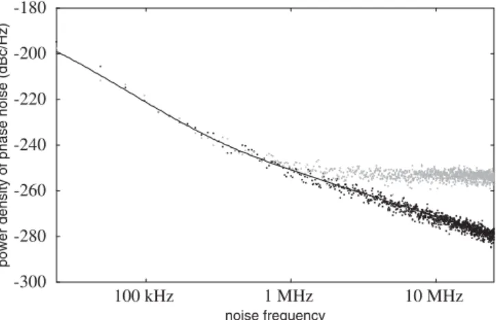
Noise of mode-locked lasers (Part I): numerical model

Thus, for type A dynamic secure zones, zone transfer security is not automatically provided for dynamically added RRs, where they could be omitted, and authentication is

Similarly, when evaluating a technology, working group participants consider IPR claims on it (including possible copyright issues with text describing it).. The issue is

The other transfer modes (Block, Compressed) do not close the connection to indicate the end of file. They have enough FTP encoding that the data connection can

A psychometric evaluation of the MENQOL was designed to assess its reliability (test-retest and internal con- sistency) and validity (face, content and construct) in women

1496 Canadian Family Physician • Le Médecin de famille canadien d VOL 50: NOVEMBER • NOVEMBRE 2004.. Letters

Now we have following result which gives a way to get back quasi coherent complexes over superscheme with a pair of quasi coherent complexes over the purely even superscheme (or

If the organization’s primary objectives are other than safeguarding intangible cultural heritage, please explain how its safeguarding objectives relate to those

As we mentioned before, if we only look for a short time solution, the fully explicit scheme for the nonlinear convection term may be analyzed accordingly as well.. Moreover,