HAL Id: hal-00706545
https://hal.archives-ouvertes.fr/hal-00706545
Submitted on 11 Jun 2012
L’Aquila earthquake inferred from cross-correlations of
ambient seismic noise.
Lucia Zaccarelli, N.M. Shapiro, L. Faenza, G. Soldati, Alberto Michelini
To cite this version:
Lucia Zaccarelli, N.M. Shapiro, L. Faenza, G. Soldati, Alberto Michelini. Variations of crustal elas-tic properties during the 2009 L’Aquila earthquake inferred from cross-correlations of ambient seis-mic noise.. Geophysical Research Letters, American Geophysical Union, 2011, VOL. 38, pp.6 PP. �10.1029/2011GL049750�. �hal-00706545�
Variations of crustal elastic properties during the 2009
1
L’Aquila earthquake inferred from cross-correlations of
2
ambient seismic noise
3
L. Zaccarelli1, N. M. Shapiro1, L. Faenza2, G. Soldati2, A. Michelini2
L. Zaccarelli, Institut de Physique du Globe de Paris, Sorbonne Paris Cité, CNRS (UMR7154),
1 rue Jussieu, 75238 Paris, cedex 5, France. ([email protected])
N.M. Shapiro, Institut de Physique du Globe de Paris, Sorbonne Paris Cité, CNRS (UMR7154),
1 rue Jussieu, 75238 Paris, cedex 5, France. ([email protected])
L. Faenza, Istituto Nazionale di Geofisica e Vulcanologia, via di Vigna Murata 605, 00143
Roma, Italy. ([email protected])
G. Soldati, Istituto Nazionale di Geofisica e Vulcanologia, via di Vigna Murata 605, 00143
Roma, Italy. ([email protected])
A. Michelini, Istituto Nazionale di Geofisica e Vulcanologia, via di Vigna Murata 605, 00143
Roma, Italy. ([email protected])
1
We retrieve seismic velocity variations within the Earth’s crust in the
re-4
gion of L’Aquila (central Italy) by analyzing cross-correlations of more than
5
two years of continuous seismic records. The studied period includes the April
6
6, 2009, Mw 6.1 L’Aquila earthquake. We observe a decrease of seismic
ve-7
locities as a result of the earthquake’s main shock. After performing the
anal-8
ysis in different frequency bands between 0.1 and 1 Hz, we conclude that the
9
velocity variations are strongest at relatively high frequencies (0.5-1 Hz)
sug-10
gesting that they are mostly related to the damage in the shallow soft
lay-11
ers resulting from the co-seismic shaking.
12
Sorbonne Paris Cité, CNRS (UMR7154),
France.
2
Istituto Nazionale di Geofisica e
1. Introduction
On April 6, 2009 a Mw 6.1 earthquake struck the central Apennines region near L’Aquila
13
(Italy) causing severe damage and more than 300 fatalities [Scognamiglio et al., 2010].
14
This area had been long recognized as seismically active [see the official seismic hazard
15
map of Italy, MPS Working Group , 2004] and an occurrence of a strong earthquake in
16
the central Apennines could not be considered as totally unexpected. Before the main
17
shock, an increase in the rate of seismicity started on September 2008 and many small size
18
events (about 300 with ML ≤ 2.5) occurred beneath the L’Aquila city area. This foreshock
19
sequence culminated with a ML = 4.1 earthquake on March 30, 2009. In the following
20
days, the seismicity decreased until two earthquakes (ML = 3.9 and ML = 3.5) occurred
21
just a few hours before the L’Aquila main shock. In agreement with the extensional
22
tectonics of the central Apennines, the focal mechanism of the L’Aquila earthquake has
23
been determined to be a normal fault on a South-West dipping plane with the rupture
24
area of ∼20x15 km2
and the dipping angle of about 50 degrees [Cirella et al., 2009]. The
25
main shock was followed by an aftershock sequence that included 33 earthquakes greater
26
than ML= 4.
27
In this study, we use a recently proposed monitoring technique based on ambient
seis-28
mic noise. The idea of this method is to use signals reconstructed from repeated
cross-29
correlations of continuous seismic records as virtual seismograms generated by highly
30
repeatable sources. In case of well distributed noise, the reconstructed virtual sources
31
are close to point forces and the cross-correlations functions can be considered as Green
32
functions [e.g., Weaver and Lobkis, 2001; Shapiro and Campillo, 2004; Sabra et al., 2005;
Shapiro et al., 2005]. Highly accurate temporal monitoring can be also performed even
34
with inhomogeneous noise sources distributions when a perfect reconstruction of the Green
35
function is not achieved [e.g., Hadziioannou et al., 2009]. The changes of the travel times
36
measured from the noise cross-correlations reflect variations of the elastic properties in
37
the propagating media, i.e., in the Earth’s crust. This approach has been recently applied
38
to monitor active volcanoes [e.g., Sens-Schönfelder and Wegler , 2006; Brenguier et al.,
39
2008a; Duputel et al., 2009; Mordret et al., 2010] and large seismogenic faults [e.g.,
We-40
gler and Sens-Schönfelder , 2007; Brenguier et al., 2008b; Chen et al., 2010] and to detect
41
seasonal changes in the Earth’s crust resulting from thermoelastic variations [e.g., Meier
42
et al., 2010].
43
In a seismogram or in a correlation function, the delay accumulates linearly with the
44
lapse time when the wave speed changes homogeneously within the medium. As a
con-45
sequence, a small change can be detected more easily when considering late arrivals.
46
This makes the use of coda waves particularly suited to measure temporal variations.
47
This can be done either by using the so-called stretching technique [e.g., Wegler and
48
Sens-Schönfelder , 2007] or with a method that was initially developed for repeated
earth-49
quakes (doublets) by Poupinet et al. [1984]. Here, we use this latter approach that has
50
been specifically adopted to make measurements from the noise cross-correlations [e.g.,
51
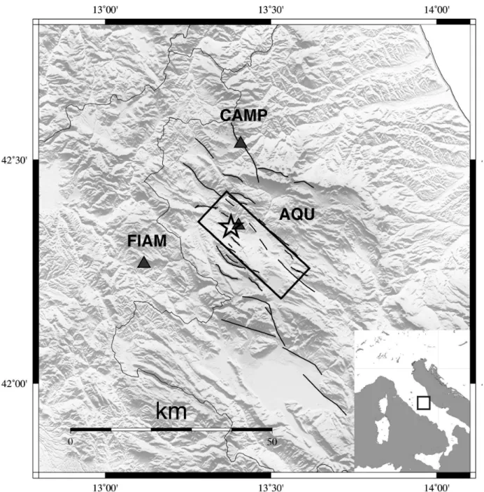
Clarke et al., 2011]. We apply this method to two years of continuous recordings by three
52
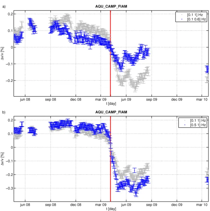
seismic stations located in the vicinity of the L’Aquila main shock fault (Figure 1) to
53
measure variations of crustal seismic velocities caused by this earthquake.
2. Selecting and pre-processing the data and computating cross-corelations
Istituto Nazionale di Geofisica e Vulcanologia (INGV) operates two large
seismologi-55
cal networks: the Italian National Seismic Network (INSN) and the Mediterranean Very
56
Broadband Seismographic Network MedNet. The INSN consists of more than 250 stations
57
with various characteristics [Amato and Mele, 2008]. MedNet consists of 22 very
broad-58
band stations distributed over the Euro-Mediterranean area with 13 of them located in
59
Italy [Mazza et al., 2008]. During period of interest for our study, four broadband stations
60
operated in continuous mode within a radius of 25 km from the main shock epicenter.
61
However, records of one of these stations contained too many gaps and we finally decided
62
to use three stations: CAMP and FIAM from INSN and AQU from MedNet (Figure 1).
63
The longest period of data availability at these three stations was between March 27, 2008
64
and April18, 2010.
65
We re-sampled time series recorded at the three stations in order to get a perfect time
66
synchronization and filled existing small gaps via a linear interpolation. Then, we
pre-67
processed the vertical component seismograms by whitening their spectra between 0.1
68
and 1 Hz and by normalizing their amplitude through a one-bit normalization. In this
69
way, the contributions arising from strong transient phenomena were reduced in both
70
time and frequency domains [e.g., Bensen et al., 2005; Brenguier et al., 2008b]. Finally,
71
we computed cross-correlations between the three pairs of stations for every hour of the
72
available recordings.
3. Measurement of seismic velocity variations
We adopted the Multi Window Cross-Spectrum (MWCS) analysis [e.g., Clarke et al.,
74
2011]. This technique was first proposed by Poupinet et al. [1984] for retrieving the relative
75
velocity variation between earthquake doublets. Brenguier et al. [2008a, b] applied this
76
technique to the cross-correlations of the seismic noise. The main idea of the method is
77
that the noise cross-correlations computed from subsequent time windows can be analysied
78
similar to records from earthquake doublets. When analyzing long time series, we compare
79
a single reference cross-correlation with many subsequent current functions. The reference
80
cross-correlation CCR for a particular station pair is obtained from stacking all available
81
cross-correlations for this pair and, therefore, is representative of the background crustal
82
state. The current cross-correlations CCC are obtained from stacking a small sub-set of
83
cross-correlations representative of a state of the crust for a given short period of time.
84
There is a trade-off between the length of the stack required to have stable estimates of
85
the CCC and the time resolution for detecting the variations. To find an optimal stacking
86
duration for the current function we tested different lengths between 10 and 100 days. For
87
each tested stacking length, we computed all possible functions CCC by applying moving
88
windows shifted by two days. Then, we computed the correlation coefficient r between the
89
reference function CCR and every CCC. The distribution of r characterizes the similarity
90
between CCR and CCC for a given stacking length. We represent the overall degree of
91
similarity by the mean and the standard deviation of this distribution. Figure 2 shows
92
these parameters for the three station pairs. We observe that the degree of similarity
increases rapidly for short stacking durations and then it tends to stabilize. We selected
94
a value of 50 days as stacking length for computing the current correlation functions.
95
The MWCS analysis consists of two computational steps [e.g., Clarke et al., 2011]. In
96
the first step, we estimate for a station pair k delay times δtk
i between CCR and CCC
97
within a set of time windows centered at ti. In case of uniform velocity perturbations,
98
the measured delays δtk
i are expected to be a linear function of time ti with a slope
99
corresponding to the relative time perturbation:
100 ∆t t = − ∆v v (1) where ∆v
v is the relative uniform seismic velocity perturbation that can be estimated in
101
the second step from a single station pair k via linear fitting of the following equation:
102 δtki = − !∆v v " k ·ti (2)
In order to obtain one estimates representative of the entire crustal volume, we merged
103
together the delays δtk
i measured from the three station pairs before proceeding with the
104
second step of the analysis. We computed the median valueδti# of the delays δtk
i for every
i-105
th window, and we inserted it into (2) to estimate of ∆v
v for the entire region encompassed
106
by the three stations. When performing this analysis, we removed the central part of
107
the cross-correlations containing direct waves (group velocities faster than 2.5 km/s; see
108
Table 1) because they may be sensitive to the changing position of the noise sources [e.g.,
109
Froment et al., 2010]. Relative velocity variations were then computed by taking into
account the coda of the cross-correlation up to a length of 60 s where the signal decreases
111
to values close to the noise level.
112
To estimate uncertainties of our measurements, we followed the method proposed by
113
Clarke et al. [2011] and performed a synthetic test on the L’Aquila noise cross-correlations.
114
We perturbed the reference cross-correlation function by stretching its waveform and
115
simulating different values of velocity variations (from 0.01% to 0.5%). Then, we added
116
a random noise with a signal-to-noise ratio of 5 (that is the mean value measured from
117
the observed cross-correlations). Finally, we applied the MWCS technique to measure the
118
apparent velocity variations ∆v
v between the perturbed cross-correlations and the original
119
CCR. The RMS deviations between the estimated velocity variations and those introduced
120
through stretching characterize the uncertainties of our measurements.
121
To investigate the depth extent of the measured crustal velocity perturbations, we
122
performed the MWCS analysis inside three different frequency bands: [0.1–1], [0.1–0.6],
123
and [0.5–1] Hz. It has been shown both theoretically and observationally that at these
124
frequencies the coda of seismograms and correlation functions are mainly composed of
125
surface waves [e.g., Hennino et al., 2001; Margerin et al., 2009]. We therefore expect that
126
the sensitivity of the coda waves to a velocity change at depth depends on their spectral
127
content with shorter periods sensitive to shallower structures and longer periods sampling
128
deeper parts of the crust. The measurement results for the three frequency bands are
129
presented in Figure 3 and show a sudden velocity decrease at the time of occurrence of
130
the L’Aquila main shock. The amplitude of this velocity drop is largest at frequencies
higher than 0.5 Hz and decreases at lower frequencies. This indicates that a large part of
132
the observed variations have their likely origin within the shallow crustal layers.
133
4. Discussion
A limited number of available stations (only three) and the fact that only
134
one of them is located in the immediate vicinity of the earthquake fault did
135
not allow us to identify exact regions that produced the observed velocity
136
variations. Also, the dataset used in this study did not allow us to make
137
robust measurements with refined time resolution. A denser network covering
138
the source area would be required to obtain better space and time resolutions
139
[e.g., Brenguier et al., 2008a]. Therefore, we interpret here only the most
140
robust average features.
141
The results presented in our study show that the L’Aquila main shock caused a
de-142
tectable reduction of seismic velocities within the surrounding crust. We observe that
143
the velocity dropped by 0.3%, which is more than 3 times larger than the fluctuations
144
observed before the main shock. Co-seismic velocity reductions can be attributed to
145
increasing crack and void densities in the shallow crustal structure and/or to reduced
146
compaction of the near-surface granular material. The presence and migration of fluids
147
can further contribute to modification of the seismic properties in the shallow crust. Our
148
results can be compared with other studies that have addressed changes of the crustal
149
parameters prior and after the L’Aquila earthquake. Amoruso and Crescentini [2010]
150
used strain measurements obtained in the Gran Sasso laboratory during the two years
151
prior to the main shock to infer that no anomalous signal was observed. They concluded
that the possible earthquake nucleation zone was confined to a volume less than 100 km3 .
153
In contrast, vp/vs anomalies have been reported by Di Luccio et al. [2010] in the weeks
154
prior to the main shock with an abrupt variation after the ML = 4.1 foreshock occured
155
on March 30. Similar results were obtained by Lucente et al. [2010] who used shear wave
156
splitting in addition to vp/vs ratios. They attribute the velocity anomalies occurring in
157
the week prior to the main shock to a complex sequence of dilatancy-diffusion processes in
158
which fluids play a key role. Terakawa et al. [2010] inverted the stress field obtained from
159
the aftershock sequence focal mechanisms to determine the fluid pressure and to conclude
160
that the spatial pattern of the sequence is driven mainly by fluid migration.
161
Our results are based on current cross-correlation functions stacked over a 50 day period
162
and, therefore, do not have the time resolution required to identify possible short-term
163
precursory variations and to separate them from the co-seismic effect. On the other hand,
164
with stacking large data volumes our estimation of the co-seismic velocity reduction is
165
inherently very robust. The observed velocity reduction is larger at higher frequencies.
166
Therefore, we prefer the hypothesis the perturbation is mainly due to damaging of shallow
167
soft sedimentary layers by the co-seismic strong ground motion [e.g., Wu et al., 2009]. This
168
effect may be also enhanced by the presence of fluids.
169
We compare the co-seismic perturbation observed during the L’Aquila earthquakes with
170
other cases when the co-seismic crustal velocity variations were measured from noise
cross-171
correlations (Table 2). The co-seismic velocity drop measured for the L’Aquila earthquake
172
(∼ 0.3%) is significantly larger than the values measured within a similar frequency band
Brenguier et al. [2008a] and Chen et al. [2010], respectively). At the same time, a stronger
175
variation (∼ 0.6%) has been observed with the stretching technique and frequencies higher
176
than 2 Hz during the Mw 6.6 Mid-Niigata earthquake. The results of this comparison
177
suggest that the level of measured co-seismic velocity variation is not a simple function of
178
the total moment release during an earthquake but is controlled by different factors such
179
as local geological conditions and, possibly, focal mechanism and source depth. Also, the
180
frequency range used in the analysis controls the depth extent of the measured anomaly.
181
Finally, the aperture of the used seismic network (i.e., the distance between the station
182
pairs) can play an important role. So far, the velocity variations reported in this study
183
were measured over a relatively large area. Therefore, they may be less sensitive to the
184
processes occurring in the immediate vicinity of the fault, where stress-induced velocity
185
perturbations are expected to be most important.
186
Acknowledgments. The data used in this study were provided by the Istituto
187
Nazionale di Geofisica e Vulcanologia. We thank G. Moguilny for maintaining the Cohersis
188
cluster on which all computations were performed. This work was supported by Agence
189
Nationale de la Recherche (France) under contract ANR-06-CEXC-005 (COHERSIS) and
190
by a FP7 ERC Advanced grant 227507 (WHISPER).
191
References
Amato, A., and F. Mele, (2008), Performance of the INGV National Seismic Network
192
from 1997 to 2007, Annals of Geophysics, 51, 417-431.
Amoruso, A., and L. Crescentini, (2010), Limits on earthquake nucleation and other
194
pre-seismic phenomena from continuous strain in the near field of the 2009 L’Aquila
195
earthquake, Geophys. Res. Lett., 37, L10307, doi:10.1029/2010GL043308.
196
Bensen, G.D., M.H. Ritzwoller, M.P. Barmin, A.L. Levshin, F. Lin, M.P. Moschetti, N.M.
197
Shapiro, and Y. Yang (2007), Processing seismic ambient noise data to obtain reliable
198
broad-band surface wave dispersion measurements, Geophys. J. Int., 169, 1239-1260,
199
doi: 10.1111/j.1365-246X.2007.03374.x.
200
Brenguier, F., M. Campillo, C. Hadziioannou, N. M. Shapiro, R. M. Nadeau, and E.
201
Larose (2008a), Postseismic relaxation along the San Andreas fault at Parkfield from
202
continuous seismological observations, Science, 321, 1478–1481.
203
Brenguier, F., N. M. Shapiro, M. Campillo, V. Ferrazzini, Z. Duputel, O. Coutant, and A.
204
Nercessian (2008b), Towards forecasting volcanic eruptions using seismic noise, Nature
205
Geoscience, 1, 126–130.
206
Chen, J. H., B. Froment, Q. Y. Liu, and M. Campillo (2010), Distribution of seismic
207
wave speed changes associated with the 12 May 2008 Mw 7.9 Wenchuan earthquake,
208
Geophys. Res. Lett., 37, L18302, doi:10.1029/2010GL044582.
209
Chiarabba, C., and 29 others (2009), The 2009 L’Aquila (central Italy) Mw
210
6.3 earthquake: Main shock and aftershocks, Geophys. Res. Lett., 36, L18308,
211
doi:10.1029/2009GL039627.
212
Cirella A., A. Piatanesi, M. Cocco, E. Tinti, L. Scognamiglio, A. Michelini, A. Lomax, and
213
E. Boschi (2009), Rupture history of the 2009 L’Aquila (Italy) earthquake from
doi:10.1029/2009GL039795.
216
Clarke, D., L. Zaccarelli , N.M. Shapiro, and F. Brenguier (2011), Assessment of resolution
217
and accuracy of the Moving Window Cross Spectral technique for monitoring crustal
218
temporal variations using ambient seismic noise, Geophys. J. Int., 186, 867-882, doi:
219
10.1111/j.1365-246X.2011.05074.x.
220
Di Luccio, F., G. Ventura, R. Di Giovambattista, A. Piscini, and F. R. Cinti (2010),
221
Normal faults and thrusts re-activated by deep fluids: the 6 April 2009 Mw 6.3 L’Aquila
222
earthquake, central Italy, J. Geophys. Res., 115, B06315, doi: 10.1029/200JB007190.
223
Duputel, Z., V. Ferrazzini, F. Brenguier, N. Shapiro, M. Campillo, and A. Nercessian
224
(2009), Real time monitoring of relative velocity changes using ambient seismic noise
225
at the Piton de la Fournaise volcano (La Reunion) from January 2006 to June 2007, J.
226
Volcanol. Geotherm. Res., 184, 164-173, doi:10.1016/j.jvolgeores.2008.11.024.
227
EMERGEO Working Group (2010), Evidence for surface rupture associated with the Mw
228
6.3 L’Aquila earthquake sequence of April 2009 (central Italy), Terra Nova, 22, 43-51.
229
Froment, B., M. Campillo, P. Roux, P. Gouedard, A. Verdel, and R.L. Weaver (2010),
230
Estimation of the effect of nonisotropically distributed energy on the apparent arrival
231
time in correlations, Geophysics, 75, SA85-SA93.
232
Hadziioannou, C., E. Larose , O. Coutant, P. Roux, and M. Campillo (2009), Stability of
233
Monitoring Weak Changes in Multiply Scattering Media with Ambient Noise
Correla-234
tion: Laboratory Experiments, J. Acoust. Soc. Am., 125, 3688–3695.
235
Hennino R., N. Trégoures, N. M. Shapiro, L. Margerin, M. Campillo, B.A. Van Tiggelen,
236
and R.L. Weaver (2001), Observation of Equipartion of Seismic Waves, Phys. Rev. Lett.,
86, 3447–3450.
238
Lucente, F. P., P. De Gori, L. Margheriti, D. Piccinini, M. Di Bona, C. Chiarabba, and
239
N. Piana Agostinetti (2010), Temporal variations of seismic velocity and anisotropy
240
before the 2009 Mw 6.3 L’Aquila earthquake, Italy, Geology, 38, 11, 1015–1018,
241
doi:10.1130/G31463.1.
242
Margerin L., M. Campillo, B. A. Van Tiggelen, and R. Hennino (2009), Energy
parti-243
tion of seismic coda waves in layered media: theory and application to Pinyon Flats
244
Observatory, Geophys. J. Int., 177, 571–585.
245
Mazza S., M. Olivieri, A Mandiello and P. Casale (2008), The Mediterranean Broad Band
246
Seismographic Network Anno 2005/06, Earthquake Monitoring and Seismic Hazard
Mit-247
igation in Balkan Countries, NATO Science Series, 81, 133-149, DOI:
10.1007/978-1-248
4020-6815.
249
Meier, U., N.M. Shapiro, and F. Brenguier (2010), Detecting seasonal variations in seismic
250
velocities within Los Angeles basin from correlations of ambient seismic noise, Geophys.
251
J. Int., 181, 985–996, doi: 10.1111/j.1365-246X.2010.04550.x.
252
Mordret, A, A.D. Jolly, Z. Duputel, and N. Fournier (2010), Monitoring of phreatic
253
eruptions using Interferometry on Retrieved Cross-Correlation Function from
Ambi-254
ent Seismic Noise: Results from Mt. Ruapehu, New Zealand, Journal of Volcanology
255
and Geothermal Research, 191, 46–59.
256
MPS Working Group (2004). Redazione della mappa di pericolosità sismica prevista
257
dall’Ordinanza PCM 3274 del 20 Marzo 2003, Rapporto Conclusivo per il
2011), INGV, Milano-Roma, 2004 April, 65 pp. including 5 appendixes.
260
Poupinet, G., W. L. Ellsworth, and J. Frechet (1984), Monitoring velocity variations in
261
the crust using earthquake doublets: an application to the Calaveras Fault, California,
262
J. Geophys. Res., 89, 5719–5731.
263
Roux, P., K. G. Sabra, P. Gerstoft, and W. A. Kuperman (2005),
P-264
waves from cross-correlation of seismic noise, Geophys. Res. Lett., 32, L19303,
265
doi:10.1029/2005GL023803.
266
Sabra, K. G., Gerstoft, P., Roux, P., Kuperman,W. A., and Fehler, M. C. (2005),
Ex-267
tracting time domain Green’s function estimates from ambient seismic noise, Geophys.
268
Res. Lett., 32, L03310.
269
Scognamiglio L., E. Tinti, A. Michelini, A. S. Dreger, A. Cirella, M. Cocco, S. Mazza, A.
270
Piatanesi (2010), Fast determination of moment tensors and rupture history: what has
271
been learned from the 6 april 2009 L’Aquila earthquake sequence, Seismol. Res. Lett.,
272
81 (6), pp. 892-906, doi:10.1785/gssrl.81.6.892.
273
Sens-Schönfelder, C. and U. Wegler (2006), Passive image interferometry and seasonal
274
variations of seismic velocities at Merapi Volcano, Indonesia, Geophys. Res. Lett., 33,
275
L21302, doi:10.1029/2006GL027797.
276
Shapiro, N. M., and M. Campillo (2004), Emergence of broadband Rayleigh waves
277
from correlations of the ambient seismic noise, Geophys. Res. Lett., 31, L07614,
278
doi:10.1029/2004GL019491.
279
Shapiro, N.M, M. Campillo, L. Stehly, and M.H. Ritzwoller (2005), High resolution surface
280
wave tomography from ambient seismic noise, Science, 307, 1615-1618.
Terakawa, T., A. Zoporowski, B. Galvan, and S. Miller, (2010), High-pressure fluid at
282
hypocentral depths in the L’Aquila region inferred from earthquake focal mechanism,
283
Geology, 38, 11, 995–998, doi:10.1130/G31457.1.
284
VanDecar, J. C., and R. S. Crosson, (1990) Determination of teleseismic relative phase
285
arrival times using multi-channel cross-correlation and lest squares, Bull. Seismol. Soc.
286
Am., 80, 1, 150–169.
287
Weaver, R. L. and O. I. Lobkis (2001), Ultrasonics without a source:
ther-288
mal fluctuation correlations at MHz frequencies, Phys. Rev. Lett., 87, 134301,
289
doi:10.1103/PhysRevLett.87.134301.
290
Wegler, U., Sens-Schönfelder C. (2007), Fault zone monitoring with passive image
inter-291
ferometry, Geophys. J. Int., 168, 1029–1033.
292
Wu, C., Z. Peng, and Y. Ben-Zion (2009), Non-linearity and Temporal Changes of Fault
293
Zone Site Response Associated with Strong Ground Motion, Geophys. J. Int., 176,
294
265-278, doi: 10.1111/j.1365-246X.2008.04005.x.
Table 1. Parameters of the three inter-stations paths used in the study. The Rayleigh wave
arrival times are roughly estimated considering a group velocity of 3 km/s [Chiarabba et al.,
2009]). Parts of the correlation functions with group velocities faster than 2.5 km/s we excluded
from the analysis to avoid the influence of the noise source variability in direct arrivals.
stations distance Rayleigh arrival cutoff
km s s
AQU_CAMP 20 6.67 ±7.5
AQU_FIAM 26 8.67 ±10
CAMP_FIAM 38 12.67 ±15
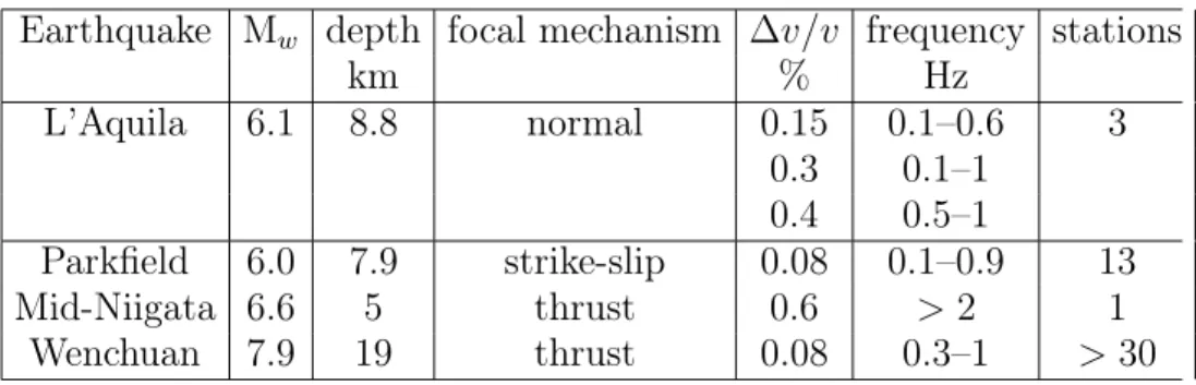
Table 2. Comparison between the L’Aquila event and other earthquakes where co-seismic
velocity variations were measured from noise cross-correlations. Values of velocity variations are
from Brenguier et al. [2008a], Wegler and Sens-Schönfelder [2007], and Chen et al. [2010], for
the Parkfield, the Mid-Niigata, and the Wenchuan earthquakes, respectively.
Earthquake Mw depth focal mechanism ∆v/v frequency stations
km % Hz L’Aquila 6.1 8.8 normal 0.15 0.1–0.6 3 0.3 0.1–1 0.4 0.5–1 Parkfield 6.0 7.9 strike-slip 0.08 0.1–0.9 13 Mid-Niigata 6.6 5 thrust 0.6 > 2 1 Wenchuan 7.9 19 thrust 0.08 0.3–1 > 30
Figure 1. Map of the central Apennines showing the location of the L’Aquila epicenter (black
20 40 60 80 100 0.85 0.9 0.95 me a n va lu e o f r CCC stacked days 20 40 60 80 100 0.02 0.03 0.04 0.05 0.06 0.07 st a n d a rd d e vi a ti o n o f r CCC stacked days AQU_CAMP AQU_FIAM CAMP_FIAM −1 0 1 C C AQU_CAMP CCR CCC (50 days) −1 0 1 C C AQU_FIAM CCR CCC (50 days) −80 −60 −40 −20 0 20 40 60 80 −1 0 1 C C t [s] CAMP_FIAM CCR CCC (50 days) r=0.96 r=0.94 r=0.92 c) d) e) b) a)
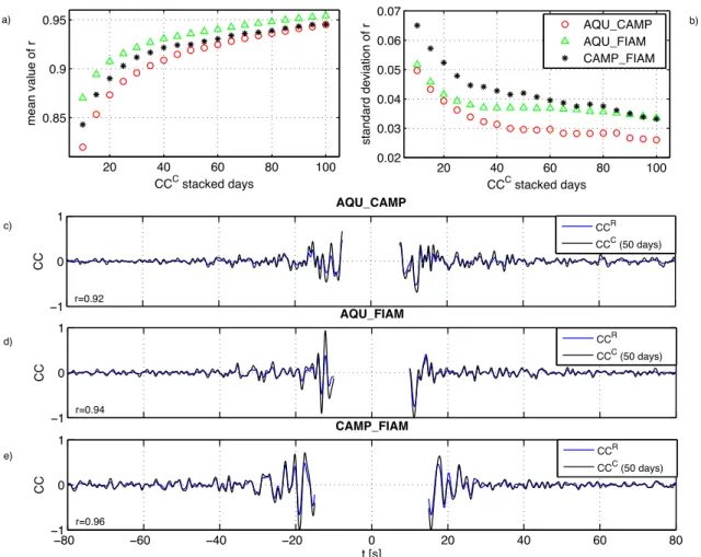
Figure 2. Mean (a) and standard deviation (b) values of the correlation coefficients r between
CCC and CCRas a function of number of days used to construct the current correlation functions
CCC. Mean and standard deviations were computed after a Fisher transformation that returns
an almost normally distributed variable [VanDecar and Crosson, 1990]. Panels (c),( d), and (e)
show the reference cross-correlation functions CCR( blue) together with an example of 50 day
current function CCC (black) for the three couples of stations. Only portions of the the signal
considered in the analysis are plotted (Table 1). Numbers in the bottom left corners are the
Figure 3. Relative velocity variations measured from cross-correlations of seismic noise
recorded at the three stations (gaps correspond to periods when the stations were not
oper-ating simultaneously). Results obtained by analyzing the whole frequency range [0.1 1] Hz are