HAL Id: hal-00296350
https://hal.archives-ouvertes.fr/hal-00296350
Submitted on 9 Oct 2007
HAL is a multi-disciplinary open access
archive for the deposit and dissemination of
sci-entific research documents, whether they are
pub-lished or not. The documents may come from
teaching and research institutions in France or
abroad, or from public or private research centers.
L’archive ouverte pluridisciplinaire HAL, est
destinée au dépôt et à la diffusion de documents
scientifiques de niveau recherche, publiés ou non,
émanant des établissements d’enseignement et de
recherche français ou étrangers, des laboratoires
publics ou privés.
overview and airborne fire emission factor measurements
R. J. Yokelson, T. Karl, P. Artaxo, D. R. Blake, T. J. Christian, D. W. T.
Griffith, A. Guenther, W. M. Hao
To cite this version:
R. J. Yokelson, T. Karl, P. Artaxo, D. R. Blake, T. J. Christian, et al.. The Tropical Forest and
Fire Emissions Experiment: overview and airborne fire emission factor measurements. Atmospheric
Chemistry and Physics, European Geosciences Union, 2007, 7 (19), pp.5175-5196. �hal-00296350�
www.atmos-chem-phys.net/7/5175/2007/ © Author(s) 2007. This work is licensed under a Creative Commons License.
Chemistry
and Physics
The Tropical Forest and Fire Emissions Experiment: overview and
airborne fire emission factor measurements
R. J. Yokelson1, T. Karl2, P. Artaxo3, D. R. Blake4, T. J. Christian1, D. W. T. Griffith5, A. Guenther2, and W. M. Hao6
1University of Montana, Department of Chemistry, Missoula, MT, 59812, USA 2National Center for Atmospheric Research, Boulder, CO, USA
3University of S˜ao Paulo, Department of Physics, S˜ao Paulo, Brazil 4University of California at Irvine, Department of Chemistry, USA
5University of Wollongong, Department of Chemistry, Wollongong, New South Wales, Australia 6USDA Forest Service, Fire Sciences Laboratory, Missoula, MT, USA
Received: 4 May 2007 – Published in Atmos. Chem. Phys. Discuss.: 23 May 2007 Revised: 20 September 2007 – Accepted: 22 September 2007 – Published: 9 October 2007
Abstract. The Tropical Forest and Fire Emissions Exper-iment (TROFFEE) used laboratory measurements followed by airborne and ground based field campaigns during the 2004 Amazon dry season to quantify the emissions from pristine tropical forest and several plantations as well as the emissions, fuel consumption, and fire ecology of trop-ical deforestation fires. The airborne campaign used an Embraer 110B aircraft outfitted with whole air sampling in canisters, mass-calibrated nephelometry, ozone by UV ab-sorbance, Fourier transform infrared spectroscopy (FTIR), and proton-transfer mass spectrometry (PTR-MS) to mea-sure PM10, O3, CO2, CO, NO, NO2, HONO, HCN, NH3,
OCS, DMS, CH4, and up to 48 non-methane organic
com-pounds (NMOC). The Brazilian smoke/haze layers extended to 2–3 km altitude, which is much lower than the 5–6 km ob-served at the same latitude, time of year, and local time in Africa in 2000. Emission factors (EF) were computed for the 19 tropical deforestation fires sampled and they largely compare well to previous work. However, the TROFFEE EF are mostly based on a much larger number of samples than previously available and they also include results for significant emissions not previously reported such as: nitrous acid, acrylonitrile, pyrrole, methylvinylketone, methacrolein, crotonaldehyde, methylethylketone, methylpropanal, “acetol plus methylacetate,” furaldehydes, dimethylsulfide, and C1
-C4alkyl nitrates. Thus, we recommend these EF for all
trop-ical deforestation fires. The NMOC emissions were ∼80% reactive, oxygenated volatile organic compounds (OVOC).
Correspondence to: R. J. Yokelson (bob.yokelson@umontana.edu)
Our EF for PM10(17.8±4 g/kg) is ∼25% higher than
previ-ously reported for tropical forest fires and may reflect a trend towards, and sampling of, larger fires than in earlier studies. A large fraction of the total burning for 2004 likely occurred during a two-week period of very low humidity. The com-bined output of these fires created a massive “mega-plume”
>500 km across that we sampled on 8 September. The mega-plume contained high PM10 and 10–50 ppbv of many
reac-tive species such as O3, NH3, NO2, CH3OH, and organic
acids. This is an intense and globally important chemical processing environment that is still poorly understood. The mega-plume or “white ocean” of smoke covered a large area in Brazil, Bolivia, and Paraguay for about one month. The smoke was transported >2000 km to the southeast while re-maining concentrated enough to cause a 3–4-fold increase in aerosol loading in the S˜ao Paulo area for several days.
1 Introduction
Biomass burning and biogenic emissions are the two largest sources of volatile organic compounds (VOC) and fine par-ticulate carbon in the global troposphere. Tropical forests produce about one-third of the global biogenic emissions and tropical deforestation fires account for much of the global biomass burning (Andreae and Merlet, 2001; Kreidenweis et al., 1999; Guenther et al., 1995, 2006). Recent estimates of the total amount of biomass burned globally vary from about 5 to 7 Pg C/y (Andreae and Merlet, 2001; Page et al., 2002). The contribution of tropical deforestation fires to total global biomass burning has been estimated as 52% (Crutzen and
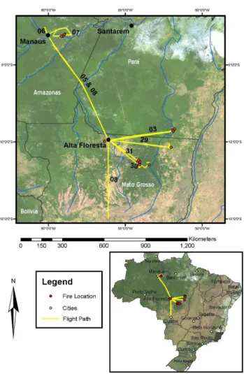
Fig. 1. The TROFFEE flight tracks and the locations of the fires
sampled.
Andreae, 1990), 34% (Hao and Liu, 1994), and 15% (An-dreae and Merlet, 2001). Thus, factors of 2–3 uncertainty need to be resolved, but these fires consistently emerge as one of the three major types of burning along with savanna fires and domestic biofuel use. A large uncertainty in the es-timated area burned is due to uncertainties in remote sens-ing applications. For example, it is unclear if small fires or understory fires can be quantified from space (Brown et al., 2006), and many fires can be missed from space due to cloud cover, which is common over tropical forested re-gions. Deforestation fires facilitate land-use change, which alters the biogenic emissions. Thus, to understand regional-global atmospheric chemistry and assess the long-term im-pact of land-use change, we must thoroughly characterize the smoke emissions from these fires and the different biogenic emissions produced by the primary forest and the various an-thropogenic “replacement” ecosystems.
The Tropical Forest and Fire Emissions Experiment (TROFFEE) provided emissions measurements for tropical deforestation fires and tropical vegetation. An overview of
TROFFEE follows. A laboratory experiment was carried out before the field campaigns that intercompared proton-transfer reaction mass spectrometry (PTR-MS), open-path Fourier transform infrared spectroscopy (FTIR), and gas chromatography (GC) coupled to PTR-MS (GC-PTR-MS) on 26 fires burning tropical fuels. The laboratory work helped plan the PTR-MS sampling protocol for the field campaign and instrumentation was available to quantify some particle characteristics not measured in the field. The GC-PTR-MS measured the branching ratios for fire-emitted species that appear on the same mass channel. The labora-tory fire and intercomparison results are presented elsewhere (Karl et al., 2007a; Christian et al., 2007a1).
The TROFFEE field campaigns were in Brazil since it has the most tropical forest and the most deforestation fires. The ground-based field campaigns included measurements of biogenic emissions from pristine forest near Manaus (Fig. 1) (Karl et al., 2007b). The ground campaign also included FTIR emissions measurements on initially-unlofted plumes from 9 biomass fires in the vicinity of Alta Floresta (Fig. 1). These plumes were due to residual smoldering combustion at deforestation sites or pasture maintenance burns or they were from charcoal kilns, cooking fires, burning dung, etc. This el-ement of TROFFEE was motivated by indications from pre-vious field campaigns that initially, unlofted biomass burn-ing plumes might contribute a large portion of the total re-gional emissions (Kauffman et al., 1998; Reid et al., 1998). The results for unlofted plumes and biofuels are described by Christian et al. (2007b). The ground campaign fires in-cluded a planned fire in which Brazilian researchers carried out a “typical” deforestation burn under conditions where the fuel consumption and other aspects of fire ecology could be measured. The emissions from this planned fire were mea-sured by the ground-based FTIR and in the TROFFEE air-borne campaign (described next).
The TROFFEE airborne campaign (Fig. 1) consisted of 44.5 flight hours between 27 August and 8 September of 2004 on an Embraer Bandeirante operated by the Brazil-ian National Institute for Space Research (Instituto Nacional de Pesquisas Espaciais (INPE)). The major instruments de-ployed on the aircraft included: (1) real-time ozone, con-densation particle counter, and mass-calibrated nephelome-try (University of S˜ao Paulo); (2) PTR-MS (National Center for Atmospheric Research); (3) Whole air sampling in can-isters with subsequent GC analysis using flame ionization, mass selective, and electron capture detection (FID, MSD, and ECD; University of California at Irvine); and (4) airborne FTIR (University of Montana). This suite of instruments was well suited for measuring CO2, CO, PM10, CH4, NOx, O3,
1Christian, T. J., Karl, T. G., Yokelson, R. J., Guenther, A., and
Hao, W. M.: The tropical forest and fire emissions experiment: Lab-oratory fire measurements and synthesis of campaign data, Atmos. Chem. Phys. Discuss., in preparation, 2007a.
Table 1. Location and characteristics of fires sampled from the INPE Bandeirante aircraft during TROFFEE 2004 airborne campaign.
Source location
Date Lat Long time period sampled Fuels observed from aircraft Fire name dd/mm dd.ddd dd.ddd LT LT
29 Aug Fire 1 29/08 −10.270 −52.159 13:41:54 14:17:10 slash under partial canopy 29 Aug Fire 2 29/08 −10.357 −52.019 14:30:37 14:43:30 Pasture
30 Aug Fire 1 30/08 −11.315 −54.064 12:56:51 13:00:45 grass and slash piles under partial canopy 30 Aug Fire 2 30/08 −11.459 −54.062 13:04:18 13:13:37 grass and slash piles under partial canopy 30 Aug Fire 3 30/08 −11.479 −54.088 13:20:14 13:20:55 grass and slash piles under partial canopy 30 Aug Fire 4 30/08 −11.491 −54.058 13:29:06 13:36:56 grass and slash piles under partial canopy
SC Fire 30/08 −11.488 −53.458 14:36:25 14:43:59 mixed forest fuels 31 Aug Fire 1 31/08 −11.282 −54.185 13:08:58 13:25:01 mixed forest fuels 31 Aug Fire 2 31/08 −11.183 −54.131 13:30:55 13:44:52 mixed forest fuels 3 Sept Fire 1 03/09 −9.224 −51.918 13:23:32 13:39:36 mixed forest fuels 3 Sept Fire 2 03/09 −9.167 −51.798 13:37:00 13:37:08 mixed forest fuels 3 Sept Fire 3 03/09 −9.311 −51.861 13:52:24 14:02:22 mixed forest fuels
3 Sept Fire 4 03/09 nm 14:13:48 14:14:16 source/fuels not observed from aircraft 3 Sept Fire 5 03/09 nm 13:22:41 13:22:54 source/fuels not observed from aircraft Planned Fire 05/09 −9.969 −56.345 14:16:42 14:51:08 mixed forest fuels
7 Sept Fire 1 07/09 −3.007 −8.930 11:49:39 11:56:42 mixed forest fuels 7 Sept Fire 2 07/09 −3.011 −58.946 12:01:13 12:01:29 mixed forest fuels 7 Sept Fire 3 07/09 −3.129 −59.056 12:04:50 12:05:58 mixed forest fuels 7 Sept Fire 4 07/09 −3.137 −59.147 12:06:46 12:07:36 mixed forest fuels
Mega-plume 08/09 nm ∼11:00 ∼12:30 source/fuels not observed from aircraft
and >40 non-methane organic compounds (NMOC) includ-ing the important biogenic emissions isoprene and methanol. In phase 1, the aircraft was based in Alta Floresta, Mato Grosso in the southern Amazon (9.917 S, 56.017 W, Fig. 1) from 27 August–5 September where the local dry/burning season was well underway. Regional haze due mostly to diluted biomass-burning smoke of unknown age and the nascent (minutes-old) emissions from 15 fires (mostly de-forestation fires) were sampled in the states of Mato Grosso and Par´a within about one-hour flight time (∼300 km) of Alta Floresta.
In phase 2, the aircraft was based in Manaus, Amazonas (3.039 S, 60.050 W, Fig. 1) from 5–8 September. The lo-cal dry season was just beginning there and the air was much cleaner and mostly unaffected by fires; especially in the mornings. The biogenic emissions were sampled from forests, several plantations east of Manaus, and the pris-tine forest at the ZF-14 tower north of Manaus. The results are discussed and integrated with the ground-based biogenic measurements by Karl et al. (2007b). In addition, four more fires were sampled around noon in the Manaus region. On 8 September from 8–13◦S we sampled a smoke plume hun-dreds of km wide that contained the combined emissions from a huge number of fires. These fires represented a sig-nificant fraction of the total Amazon burning for 2004 and they generated a “mega-plume,” which we discuss in detail in Sect. 3.4. All the fires sampled are listed in Table 1. The
TROFFEE flight tracks and individual fires are mapped in Fig. 1. A more detailed map of the 6–7 September flights is given by Karl et al. (2007b).
The fire component of TROFFEE is covered in four ini-tial papers. The lab fire results and the chemistry and im-pact of unlofted smoke not amenable to airborne sampling are covered in two papers (Christian et al., 2007a1, b). Karl et al. (2007a) present the instrument intercomparison and the emission ratios of many VOC to acetonitrile, which is thought to be mostly emitted by biomass burning. The main focus of this paper is to provide background on the region and experiment and to detail the airborne measurements of fire emission factors, which are needed as model input and for bottom-up emissions estimates at any scale. Some aspects of the airborne measurements in clean air (relatively unaf-fected by fires) and haze (dilute/aged smoke) are also given to clarify the regional atmospheric conditions and make our fire-sampling strategy clear.
A major goal of all the TROFFEE fire research was com-prehensive sampling of reactive species as close as possible to the source. The rationale for this is given next. Much of the initial interest in fires focused on the climate forc-ing. In fact, in El-Ni˜no years, the carbon added to the at-mosphere by biomass burning may exceed that from fossil fuels (Page et al., 2002). The CO2due to tropical
deforesta-tion alone may cause an average annual amount of warming that is 20–60% of that caused by the CO2 from all global
industry (Crutzen and Andreae, 1990) and fires emit more other greenhouse gases (GHG) per CO2than fossil fuel use
(Christian et al., 2003). Photochemical processing of fire emissions was shown to produce O3 (Fishman et al., 1991;
Andreae et al., 1994), an important GHG (Prather et al., 1994). Particles emitted by fires were found to cause neg-ative forcing both directly (Hobbs et al., 1997) and indirectly by reducing cloud droplet sizes and increasing cloud albedo (Kaufman and Fraser, 1997).
In recent years, the reactivity and the rapid post-emission chemistry of smoke have attracted increasing attention. Early laboratory and field studies of biomass burning had concen-trated on measuring the emissions of CO2, CO, NOx, and
hydrocarbons (Lobert et al., 1991; Blake et al., 1996; Ferek et al., 1998), but later laboratory work showed that 60–80% of the NMOC emissions from fires were actually highly reac-tive, oxygenated VOC (OVOC) (Yokelson et al., 1996, 1997; Holzinger et al., 1999). The dominance of NMOC emissions by OVOC was then confirmed for all of the major types of biomass burning except tropical forest fires: e.g. savannas, biofuels, agricultural waste, peat, and boreal forest (Goode et al., 2000; Christian et al., 2003; Bertschi et al., 2003a). In ad-dition, field measurements of rapid changes in smoke plume chemistry became available (Goode et al., 2000; Yokelson et al., 2003a; Hobbs et al., 2003). Detailed photochem-ical smoke models reproduced the observed O3 formation
rate in only some cases and were unable to predict the ob-served formation of other species such as acetone and acetic acid (Mason et al., 2001; Jost et al., 2003; Tabazadeh et al., 2004; Trentmann et al., 2005). Sensitivity analysis showed that model performance was significantly enhanced by us-ing more complete information on the initial NMOC (mostly OVOC) emissions. About 80% of biomass burning occurs in the tropics, which govern the oxidizing power of the global troposphere (Crutzen and Andreae, 1990). Fires are a major source of CO (the main sink of OH), but the large quantities of OVOC emitted by fires, and the secondary O3, are HOx
(OH+HO2) precursors and important oxidants
(Finlayson-Pitts and (Finlayson-Pitts 1986; Singh et al., 1995). Thus there was a critical need for the first-ever data on OVOC emissions from tropical deforestation fires.
2 Experimental details 2.1 Instrument details
2.1.1 Airborne FTIR (AFTIR) and whole air sampling in canisters
The basic design and operation of the AFTIR system has been described in detail by Yokelson et al. (1999, 2003a, b). A summary description is given here followed by the details of how AFTIR was used to fill canisters. The AFTIR has a dedicated, halocarbon-wax, coated inlet that directs ram air
through a Pyrex, multipass cell. Infrared spectra of the cell contents are acquired continuously (every 0.83 s) throughout each flight and the flow-control valves are normally open, which flushes the cell with outside air every 2–4 s. The fast-acting flow control valves allow the system flow to be tem-porarily stopped for signal averaging and improved accuracy on “grab samples.” The IR spectra are later analyzed to quan-tify the compounds responsible for all the major peaks. This accounts for most of the trace gases present in the cell above 5–20 ppbv (Goode et al., 1999).
For TROFFEE, a Teflon valve was added to the AFTIR cell that connected to two options for filling evacuated can-isters. For a canister sample of a plume, we used a teflon-diaphragm pump to pressurize the can with gas from the AFTIR cell, which already contained a grab sample of the plume. Pressurizing the cans allows more sensitive and/or a wider variety of analyses and also prevents contamination in the event of a slow leak. Operationally-simpler canister sam-ples of background air were obtained by diverting a portion of the flow through the AFTIR cell into the cans. The .635 cm outside diameter Teflon tubing connecting to the canisters had a pressure higher than the cabin pressure and attached to the can with Ultra-Torr® fittings. We flushed the connecting tubing with cell air by loosening the fitting for a few min-utes. Once the fitting was retightened the pre-evacuated can was opened and filled to cell pressure within seconds. The filling time of each can was shown by a sharp, (logged) pres-sure response in the AFTIR cell. The canisters were later analyzed at UCI using GC/FID-MSD-ECD (Colman et al., 2001).
2.1.2 IR spectral analysis
Mixing ratios for H2O, CO2, CO, and CH4 were obtained
by multicomponent fits to sections of the IR transmission spectra with a synthetic calibration non-linear least-squares method (MALT 5.2) recently developed by one of the au-thors (Griffith). To derive excess mixing ratios (1X) for the above species in smoke plumes we took the mixing ratio of the species “X” in the smoke plume grab sample minus the mixing ratio of X in the closest grab sample of background air. The use of a nearby background sample for this subtrac-tion is important because it excludes the contribusubtrac-tion of the aged smoke that contributes much of the background air in areas heavily impacted by biomass burning.
We used the same background-plume spectra pairs to gen-erate absorbance spectra of the smoke plume samples. Ex-cess mixing ratios are retrieved directly from the absorbance spectra (Hanst and Hanst, 1994). Excess mixing ratios for NO and NO2in smoke plumes were obtained from the
ab-sorbance spectra using peak integration and a multipoint cal-ibration. Excess mixing ratios for ethylene (C2H4),
acety-lene (C2H2), propylene (C3H6), methanol (CH3OH), formic
acid (HCOOH), acetic acid (CH3COOH), ammonia (NH3),
(O3)were retrieved from the absorbance spectra by spectral
subtraction (Yokelson et al., 1997). The spectral subtraction routine used commercial IR reference spectra or multiple ref-erence spectra per species that we recorded in house for NH3,
CH3OH, CH3COOH, C2H4, and C3H6. Excess mixing
ra-tios for C2H6and HCHO were retrieved from the absorbance
spectra using MALT 5.2. For most compounds the detection limit was 5–10 ppbv, but for NOx, HCHO, acetic acid, C3H6,
C2H6, and O3it was ∼15–20 ppbv.
The spectral analysis routines were challenged by apply-ing them to IR spectra of over 50 flowapply-ing standard mixtures. The routines typically returned values within 1% of the nom-inal, delivered amount. Consideration of the accuracy of the standards, flow meters, and other issues suggests that the ab-solute accuracy of our mixing ratios is ±1–2% for CO2, CO,
and CH4and ±5% (1σ ) or the detection limit, whichever is
larger, for the other compounds. NH3 was the only
com-pound noticeably affected by brief storage in the cell, but the NH3 values have been corrected both for initial passivation
of the cell and slow decay during grab-sample storage as de-scribed by Yokelson et al. (2003b) and should be accurate to
±10% or the detection limit. 2.1.3 PTR-MS
A detailed description of the PTR-MS instrument is given elsewhere (Lindinger et al., 1998). Briefly, H3O+ ions are
used to ionize volatile organic compounds (VOC) via proton-transfer reactions. The value for E/N (E the electric field strength and N the buffer gas density) in the drift tube was kept at about 123 Townsend, which is high enough to avoid strong clustering of H3O+ ions with water and thus a
hu-midity dependent sensitivity. The sensitivity of the PTR-MS instrument during this study was typically on the order of 70 Hz/ppbv (counts per second per ppbv) for acetone and 50 Hz/ppbv for methanol at 2.3 mbar buffer gas pressure with a reaction time of 110 µs and 3–4 MHz H3O+ions, and thus
inferred a signal to noise ratio of 60% at a concentration of 20 pptv and a 2 s integration time. The PTR-MS sampled air through a dedicated, rear-facing, Teflon inlet. About 17 mass channels were monitored during flight with a measurement period for each species of 1–20 s. Higher sampling rates were used in the plumes. More details about the PTR-MS in this campaign are given by Karl et al. (2007a).
2.1.4 Particle, ozone, and auxiliary measurements
A list of the instruments deployed by the University of S˜ao Paulo and their measurement frequency follows. (1) DataRAM4 (Thermoelectron Corp), which measures the mass of particles with an aerodynamic diameter <10 mi-crons (PM10) and mean particle diameter (microns) at 0.5 Hz.
(2) 3-channel nephelometer (RBG) at 0.2857 Hz. (3) 7-channel aethalometer (Magee Scientific) measuring particle absorbance from 950–450 nm every 2 min. (4) Ozone by UV
absorbance (1 min time resolution). (5) GPS (Garmin) mea-suring UTC time, latitude, longitude, and altitude at 1 Hz. Instruments 1–4 had specialized inlets located on the front belly of the aircraft adjacent to the PTR-MS inlet. The PM10 measurements reported here were measured by the
DataRAM4, which is a two-wavelength nephelometer with a built in humidity correction. The instrument has been run side by side with a TEOM (Tapered Element Oscillating Mi-crobalance) under smoky conditions in the Amazon and good agreement was observed.
2.1.5 Flight plans and sampling protocols
While based in Alta Floresta (27 August–5 September) back-ground air (defined here as air not within a visible biomass burning plume) was characterized at various altitudes (up to 3352 m). These were afternoon flights conducted to search for and sample fires and most of the measurements were made below the top of the (hazy) mixed layer. While based in Manaus cleaner background air was sampled during morn-ing flights over a similar altitude range. The Manaus flights included both continuous-spiral and “parking-garage”-type vertical profiles over the instrumented ZF-14 Tower and a constant-altitude “racetrack” pattern that sampled several re-gionally important ecosystems (undisturbed forest, flooded forest, and various plantations) east of Manaus (Karl et al., 2007b). When sampling background air in either region, the PTR-MS continuously cycled through a suite of mass chan-nels with a resulting measurement frequency for individual species ranging from 10–20 s. Overall, twenty-one canisters were used to “grab” background samples at key locations. The airborne FTIR (AFTIR) was operated either continu-ously (time resolution of 0.83 to 18 s) or to acquire 133 grab samples of background air.
To measure the initial emissions from fires in both regions, we sampled smoke less than several minutes old by pene-trating the column of smoke 200–1000 m above the flame front. The AFTIR system and cans obtained grab samples in the plume (and paired background samples just outside the plume). The other instruments measured their species continuously while passing through the plume. More than a few kilometers downwind from the source, smoke plume samples are “chemically aged” and better for probing post-emission chemistry than estimating initial post-emissions (Hobbs et al., 2003; de Gouw et al., 2006).
2.2 Data processing and synthesis
Grab samples or profiles of an emission source can provide excess mixing ratios (1X, see Sect. 2.1.2). 1X reflect the instantaneous dilution of the plume and the instrument re-sponse time. Thus, a widely used, derived quantity is the normalized excess mixing ratio where 1X is compared to a simultaneously measured plume tracer such as 1CO or
1CO2. A measurement of 1X/1CO or 1X/1CO2made in
a nascent plume (seconds to a few minutes old) is an emission ratio (ER). The ER 1CO/1CO2 and the modified
combus-tion efficiency (MCE, 1CO2/(1CO2+1CO)) are useful to
indicate the relative amount of flaming and smoldering com-bustion for biomass burning. Higher 1CO/1CO2or lower
MCE indicates more smoldering (Ward and Radke, 1993). For any carbonaceous fuel, a set of ER to CO2for the other
major carbon emissions (i.e. CO, CH4, a suite of NMOC,
particulate carbon) can be used to calculate emission factors (EF, g compound emitted/kg dry fuel) for all the gases quan-tified from the source using the carbon mass-balance method (Yokelson et al., 1996). EFs are combined with fuel con-sumption measurements to estimate total emissions at vari-ous scales. In this project, the primary data needed to calcu-late EF was provided by AFTIR measurements of CO2, CO,
CH4, and many NMOC. However, the PTR-MS and canister
sampling added numerous, important NMOC that were be-low AFTIR detection limits or not amenable to IR detection. The PM10data allowed inclusion of particle carbon. Next we
summarize the methods we used to calculate ER and EF and to couple/synthesize the data from the various instruments on the aircraft.
2.2.1 Estimation of fire-average, initial emission ratios (ER)
The first step in our analysis was to compute molar ER to CO and CO2for each species detected in the AFTIR or can grab
samples; and molar ER to methanol (justified below) for each species detected by PTR-MS. This is done for each individ-ual fire or each group of co-located, similar fires. If there is only one sample of a fire (as for the canisters) then the calcu-lation is trivial and equivalent to the definition of 1X given above. For multiple AFTIR grab samples of a fire (or group of fires) then the fire-average, initial ER were obtained from the slope of the least-squares line (with the intercept forced to zero) in a plot of one set of excess mixing ratios versus another (see Figs. 2a and b). This method is justified in de-tail by Yokelson et al. (1999). We calculated the fire-average MCE for each fire using the fire-average 1CO/1CO2and the
equation MCE=1/((1CO/1CO2)+1).
The ER for PTR-MS compounds with respect to methanol were obtained by similar plots except that the integrated ex-cess mixing ratios (ppbv s) for each pass thru the plume were used in lieu of the individual excess mixing ratios (see Fig. 2c). Comparison of integrals provides more accurate ER (Karl et al., 2007a). When two or more compounds appear on the same mass channel, the signal was assigned to each com-pound using the branching ratios measured by GC-PTR-MS in smoke from tropical fuels burned during the lab experi-ment. This adds additional uncertainty for these compounds since these branching ratios typically varied by 10–20% from fire to fire during the lab experiments (Karl et al., 2007a).
The ER to CO for the NMOC detected by PTR-MS was derived from a simple two step process. The process is based
on the fact that we have found excellent agreement between FTIR and PTR-MS for methanol, over a wide range of con-centrations, in two other studies (Christian et al., 2004; Karl et al., 2007a). An example of the process follows. The ER for acetaldehyde to CO was taken to be the PTR-MS ER “ac-etaldehyde/methanol” times the AFTIR ER “methanol/CO.” Multiplying again by the AFTIR CO/CO2ratio gave the
ra-tio of the NMOC to CO2 – as needed for the EF
calcula-tion. A slightly different approach was needed to couple the data from the particle instruments. The DataRAM4 measures the STP-equivalent PM10per unit volume (µg/m3)every two
seconds while passing thru a plume. We converted the inte-grated methanol mixing ratios to an inteinte-grated mass (STP) of methanol and ratioed the integrated particle mass to this (see Fig. 2d).
2.2.2 Estimation of fire-average, initial emission factors We estimated fire-average, initial EF for PM10and each
ob-served trace gas from our fire-average, initial ER using the carbon mass balance method (Ward and Radke, 1993) as de-scribed by Yokelson et al. (1999). Briefly, we assume that all the volatilized carbon is detected and that the fuel car-bon content is known. For purposes of the carcar-bon mass bal-ance we assume the particles are 60% C by mass (Ferek et al., 1998). By ignoring unmeasured gases we are probably inflating the emission factors by 1–2% (Andreae and Mer-let, 2001). We assumed in our EF calculations that all the fires burned in fuels containing 50% carbon by mass. This is in good agreement with previous studies of tropical biomass (Susott et al., 1996), but the actual fuel carbon percentage may vary by ±10% (2σ ) of our nominal value. (Emission factors scale linearly with assumed fuel carbon percentage.) 2.3 Overview of Brazilian fires and the fires sampled in the
airborne campaign
2.3.1 General fire characteristics relevant to sampling strategies
Conversion of the Amazon primary forest usually starts at the beginning of the dry season (May–July) when the biomass is slashed and dried (Fearnside, 1993). Most of the burns oc-cur late in the dry season (August–October) to achieve high consumption. A typical burn is initiated by starting a line of flame along the outer edge of the slashed area. As the flame front propagates inward, the flame-induced convection col-umn entrains the emissions from both flaming combustion and any nearby smoldering combustion. These emissions can be sampled from an aircraft. In some cases, smoldering can continue after the convection envelope has moved too far away to entrain the emissions or convection from the en-tire site has ceased. When either of these conditions is met, we term this residual smoldering combustion (RSC). RSC emissions are not initially lofted or amenable to airborne
y = 0.0561x R2 = 0.9828 0 1 2 3 4 5 6 7 8 0 50 100 150 ΔCO2 (ppm) Δ C O (p p m ) (a) y = 0.0329x R2 = 0.9365 0 0.05 0.1 0.15 0.2 0.25 0 2 4 6 8 ΔCO (ppm) Δ C H3 O H (p p m ) (b)
y = 0.4138x
R
2= 0.9771
0
100
200
300
400
500
600
0
500
1000
1500
ΔCH
3OH (ppb s)
Δ
C
H
3C
H
O
(p
p
b
s
)
(c)
y = 5.9877x R2 = 0.9132 0 5000 10000 15000 20000 25000 30000 35000 40000 0 2000 4000 6000 ΔCH3OH (ug/m 3 s) Δ PM1 0 (u g /m 3 s ) (d)Fig. 2. Examples of the plots used to derive emission ratios (ER) in this work. See Sect. 2.2.1 for details. (a) plot used to derive the
ER 1CO/1CO2from AFTIR grab samples of the 5 September planned fire. (b) as in a for the ER 1CH3OH/1CO. (c) plot for the ER
1CH3CHO/1CH3OH from integrated PTR-MS traces during plume penetrations of the 5 September fire. (d) plot used to derive the ER
1PM10/1CH3OH (mass ratio) from integrated PTR-MS and nephelometer traces during plume penetrations of the shifting cultivation fire
on 30 August.
sampling. When dry, large-diameter fuels are present RSC may account for a large part of the total biomass consumed (Bertschi et al., 2003b; Kauffman et al., 1998).
2.3.2 Overview of Brazilian biomass burning
This section summarizes Brazilian biomass burning to help assess the representativeness of the fires we actually sampled. Brazil contains ∼2×10⁶km2 of savanna (cerrado), mostly in southern Brazil, which is burned every 1–3 years in fires that rapidly consume 5–10 Mg/ha of mostly fine fuels such as grass (Coutinho, 1990; Ward et al., 1992; Kauffman et al., 1994; Andrade et al., 1999). For estimating the emissions
from any global savanna fire, we recommend the tables for savanna fires in Christian et al. (2003) and Andreae and Mer-let (2001).
Brazil has ∼4×10⁶km2 of evergreen tropical forest mostly in the Amazon basin, which represents ∼25% of the world’s total “rainforest.” Deforestation rates in the Amazon since 1978 ranged from 11–29×103km2/y (http://www.obt. inpe.br/prodes/). About 85% of the cumulative deforested area for 1978–2005 occurred in the rapidly developing south-ern and eastsouth-ern edges of the Amazon basin where the states of Par´a and Mato Grosso are located (Fig. 1). Deforesta-tion fires involve large total aboveground biomass (TAGB)
loading averaging ∼300 Mg/ha of which ∼40% is consumed by the fires for a total fuel consumption of ∼120 Mg/ha. (Ward et al., 1992; Fearnside et al., 1993; Carvalho et al., 1998, 2001; Guild et al., 1998).
Pastures established in previously forested areas of the Amazon are maintained by burning every 2–3 years (Guild et al., 1998). The TAGB can be quite large partly because resid-ual wood debris (RWD) persists for many years. Reported TAGB ranges from 119 Mg/ha (87% RWD) to 53 Mg/ha (47% RWD) in pastures 4–20 years old (Barbosa and Fearn-side, 1996; Guild et al., 1998; Kauffman et al., 1998). Large-diameter RWD accounted for ∼45% of the fuel consumption in the above studies. Until recently, nearly all deforested ar-eas in the Brazilian Amazon were eventually converted to pasture and the total emissions from Brazilian pasture fires are thought to be comparable to the total emissions from Brazilian deforestation fires (Fearnside, 1990; Barbosa et al., 1996; Kauffman et al., 1998). Globally, deforestation fires associated with shifting cultivation and plantation establish-ment dominate and pasture fires are relatively less common.
Brazil has recently seen explosive growth in large-scale, mechanized agriculture, especially in Mato Grosso (Cardille and Foley, 2003). Both pastures and forest are converted to croplands for (mostly) soy. In either case, all large-diameter fuels must be removed by the burns. Morton et al. (2006) found that Mato Grosso accounted for 40% of the new defor-estation in Amazonia from 2000–2004. Within Mato Grosso from 2001–2004, pasture was still the main use following de-forestation, but that fraction was decreasing and direct tran-sition to large areas of cropland accounted for 23–28% of de-forestation. Thus, we conclude that the expansion of mecha-nized agriculture could imply an increase in both the area of individual fires and the fuel consumed per unit area.
A few other less dominant fire-types occur in Brazil. Sec-ondary forests are used in similar fashion to primary forests (Fearnside, 1990, 2000). Lower intensity fires occur natu-rally in seasonally dry forests, such as the Caatinga in eastern Brazil and these forests are also subject to land-use change (Kauffman et al., 1993). Selective logging promotes fire sus-ceptibility and is increasing in the Amazon (Grainger, 1987; Kauffman and Uhl, 1990; Cochrane et al. 1999; Laurance, 2000).
As discussed in detail by Christian et al. (2007b), RSC could produce a large part of the Amazonian fire emissions and this motivated our simultaneous airborne and ground based campaigns. However, RSC likely occurs mostly on pasture maintenance fires rather than the deforestation fires, which were our main target.
2.3.3 Description of the fires sampled in the airborne cam-paign
Nearly all the fires we observed in Mato Grosso and southern Par´a were related to the expansion of exist-ing, large farms or ranches (Table 1). All but 3 of
these fires were located on the edge of forested areas that were adjacent to large tracts of cleared, often culti-vated, land. Casual examination of MODIS visible im-ages of this region reveals that nearly all hotspots are lo-cated at the edge of dark-green (forested) areas, adjacent to light-green (cleared) areas (http://rapidfire.sci.gsfc.nasa.gov/ subsets/?AERONET Alta Floresta/2004252). However, the second fire sampled on 29 August was in a grass meadow and no large fuels were visible from the air. This was probably a maintenance fire for an older pasture. The other exception was two small fires observed on 31 August adjacent to the Xingu River in the center of an indigenous reserve and far from any visible clearings or roads. These fires were likely due to shifting cultivation and the one we sampled is labeled the “SC” fire in Tables 1 and 2. Complete burning of logging slash to prepare for mechanized agriculture can be promoted by bulldozing the fuel into long piles (“windrows”) that were observed from the aircraft on at least one group of fires (30 August Fires 1–4). In all areas, the fires frequently occurred in clusters.
TROFFEE supported a planned, deforestation fire on a farm near Alta Floresta under the supervision of Jo˜ao Car-valho (University of Estadual Paulista) and Ernesto Alvarado (University of Washington). Measurements included fuel consumption, charcoal production, propagation of smolder-ing combustion, forest flammability adjacent to clearcuts, on-site meteorology, fire effects on groundwater chemistry, and recovery and regeneration of burned areas. The emissions from this fire were sampled by ground-based FTIR (Chris-tian et al., 2007b) and the TROFFEE aircraft (5 September data in Tables 1 and 2). In summary, pasture fires were undersampled relative to their importance in Brazil, but we achieved our objective of comprehensive chemical sampling of the emissions from deforestation fires, which are far more significant globally.
3 Results and discussion
3.1 Characteristics of clean background air
We briefly summarize some of the data obtained in early dry season, clean air near Manaus (see also Karl et al., 2007b). These data are of intrinsic interest and by comparison to data from the more active burning region further south (Sect. 3.2), they highlight the degree to which fires can perturb back-ground air over a large geographic area. Figure 3a shows all the AFTIR CO grab samples from 6 and 7 September, obtained in the Manaus region, which was not visibly im-pacted by a biomass burning haze before noon. The CO av-erage was 134±13 ppbv. This is a relatively narrow range. Chou et al. (2002) measured numerous CO vertical profiles in nearly the same location in April–May 1987. Their fig-ures indicate that their CO values averaged about 100 ppb. The larger values we observed could be due to a gradual
Table 2. Initial emission factors for the fires sampled at their source during the 2004 TROFFEE airborne campaign. Effective emission
factors for the mega-plume, which was sampled downwind from source.
29 Aug 29 Aug 30 Aug 30 Aug 31 Aug 31 Aug 3 Sep 5 Sep 7 Sep 8 Sep
Fire 1 Fire 2 Fires 1–4 SC Fire Fire 1 Fire 2 Fires 1–5 Planned Fires 1–4 Study Standard Mega-Plume MPEEF-Fire average deviation averagec Compound EF EF EF EF EF EF EF EF EF EF EF Effective EF formula or name g/kg g/kg g/kg g/kg g/kg g/kg g/kg g/kg g/kg g/kg g/kg g/kg # stdev’s
AFTIR species CO2 1638 1591 1567 1579 1603 1636 1579 1679 1662 1615 40 1651 0.91 CO 95.72 112.08 133.45 124.82 110.70 93.13 110.52 59.91 72.36 101.41 23.78 87.54 −0.58 MCE 0.916 0.900 0.882 0.890 0.902 0.918 0.901 0.947 0.936 0.910 0.021 0.923 0.61 NO 0.283 nmb 0.281 0.514 0.208 0.438 0.746 2.681 nm 0.74 0.877 2.297 1.78 NO2 1.979 0.930 1.157 0.509 0.738 2.216 1.393 3.441 4.120 1.83 1.245 1.899 0.05 NOx(as NO) 1.574 0.606 1.035 0.846 0.690 1.883 1.654 4.926 2.687 1.77 1.359 3.535 1.30 HONO 0.345 0.167 nm nm nm nm nm nm nm 0.26 0.126 nm nm CH4 4.213 6.916 5.751 7.544 5.323 5.486 7.220 3.353 5.324 5.68 1.380 7.636 1.42 C2H4 0.747 1.238 0.958 1.215 0.997 0.809 1.520 0.642 0.454 0.95 0.332 0.378 −1.73 C2H2 0.094 nm 0.083 0.101 0.140 0.084 0.172 0.923 0.620 0.28 0.317 0.085 −0.61 C2H6 0.548 1.137 0.917 1.157 0.893 0.532 1.478 nm nm 0.95 0.341 nm nm C3H6 0.452 0.728 0.424 0.606 0.462 0.317 0.509 0.091 nm 0.45 0.190 nm nm HCHO 1.277 1.912 1.674 1.783 1.445 1.517 2.201 1.741 1.409 1.66 0.286 1.004 −2.30 CH3OH 2.077 2.874 2.724 3.371 2.294 2.331 3.002 2.252 2.165 2.57 0.445 2.550 −0.04 CH3COOH 3.134 4.172 3.635 3.590 2.643 3.232 3.190 3.579 3.704 3.43 0.436 9.242 13.33 HCOOH 0.398 0.519 0.377 0.223 0.246 0.508 0.323 0.978 1.715 0.59 0.479 3.266 5.59 NH3 1.127 1.364 1.093 1.769 0.653 0.658 1.476 1.236 0.308 1.08 0.460 1.509 0.94 HCN 0.665 0.537 0.699 0.582 0.486 0.409 0.426 2.098 0.184 0.68 0.555 0.169 −0.91 PTR-MS species and PM10 acetonitrile 0.574 0.276 0.270 0.381 0.291 0.347 0.485 0.359 0.336 0.37 0.101 nm nm acetaldehyde 1.255 1.202 1.167 1.240 0.751 1.041 3.322 1.282 1.202 1.38 0.745 nm nm acrylonitrile 0.051 nm 0.038 nm 0.020 0.048 nm nm nm 0.04 0.014 nm nm acrolein nm nm nm nm 0.306 0.477 nm 0.808 0.732 0.58 0.232 nm nm acetonea 0.429 0.525 0.645 0.673 0.235 0.506 0.803 0.694 0.590 0.57 0.167 nm nm propanala 0.067 0.082 0.101 0.105 0.037 0.079 0.126 0.109 0.092 0.09 0.026 nm nm isoprenea 0.236 0.366 0.402 0.396 0.271 0.296 0.625 0.378 0.386 0.37 0.112 nm nm furana 0.207 0.320 0.352 0.347 0.237 0.259 0.547 0.331 0.338 0.33 0.098 nm nm methylvinyl ketonea 0.166 0.499 0.340 nm 0.399 0.318 0.215 0.411 0.436 0.35 0.113 nm nm methacroleina 0.066 0.198 0.135 nm 0.158 0.126 0.085 0.163 0.173 0.14 0.045 nm nm crotonaldehydea 0.100 0.302 0.205 nm 0.241 0.192 0.130 0.248 0.263 0.21 0.068 nm nm methylethyl ketonea 0.229 0.469 nm nm nm nm 0.654 nm nm 0.45 0.213 nm nm methyl propanala 0.081 0.165 nm nm nm nm 0.230 nm nm 0.16 0.075 nm nm acetol and methylacetate nm nm 0.649 nm 0.840 0.607 0.895 0.700 0.627 0.72 0.120 nm nm benzenea 0.189 0.381 0.168 nm 0.538 0.176 0.234 0.261 0.172 0.26 0.131 nm nm C6carbonyls 0.098 0.307 0.105 nm Nm nm 0.241 0.363 0.159 0.21 0.109 nm nm 3-methylfurana 0.252 0.707 0.434 nm 0.843 0.389 0.668 0.511 0.413 0.53 0.196 nm nm 2-methylfurana 0.036 0.101 0.062 nm 0.120 0.056 0.095 0.073 0.059 0.08 0.028 nm nm hexanala 0.006 0.017 0.010 nm 0.020 0.009 0.016 0.012 0.010 0.01 0.005 nm nm 2,3 butanedionea 0.317 0.790 0.509 nm 0.855 0.490 0.995 0.634 0.659 0.66 0.219 nm nm 2-pentanonea 0.032 0.085 0.052 nm 0.094 0.051 0.106 0.066 0.069 0.07 0.024 nm nm 3-pentanonea 0.014 0.038 0.023 nm 0.042 0.023 0.047 0.029 0.031 0.03 0.011 nm nm toluene 0.102 0.109 0.126 nm 0.227 0.096 0.399 0.135 0.368 0.20 0.123 nm nm phenola nm nm nm nm nm nm nm 0.406 0.282 0.34 0.088 nm nm other substituted furans nm nm nm nm nm nm nm 1.095 1.071 1.08 0.016 nm nm furaldehydes nm nm nm nm nm nm nm 0.255 0.256 0.26 0.001 nm nm xylenesa 0.086 0.092 0.076 nm 0.132 0.060 0.322 0.137 0.115 0.13 0.083 nm nm ethylbenzenea 0.053 0.084 0.047 nm 0.118 0.044 0.126 0.078 0.052 0.08 0.033 nm nm PM10 17.61 14.43 17.94 20.18 19.81 17.27 26.41 12.53 14.28 17.83 4.121 nm nm UCI-Canister species OCS nm nm nm nm nm nm nm 0.0247 nm 0.0247 nm nm nm DMS nm nm nm nm nm nm nm 0.0022 nm 0.0022 nm nm nm CFC 12 nm nm nm nm nm nm nm 0.0028 nm 0.0028 nm nm nm MeONO2 nm nm nm nm nm nm nm 0.0163 nm 0.0163 nm nm nm EtONO2 nm nm nm nm nm nm nm 0.0057 nm 0.0057 nm nm nm i-PrONO2 nm nm nm nm nm nm nm 0.0010 nm 0.0010 nm nm nm n-PrONO2 nm nm nm nm nm nm nm 0.0003 nm 0.0003 nm nm nm 2-BuONO2 nm nm nm nm nm nm nm 0.0006 nm 0.0006 nm nm nm C2H6 nm nm nm nm nm nm nm 0.5600 nm 0.5600 nm nm nm 1-Butene nm nm nm nm nm nm nm 0.0200 nm 0.0200 nm nm nm trans-2-Butene nm nm nm nm nm nm nm 0.0161 nm 0.0161 nm nm nm cis-2-Butene nm nm nm nm nm nm nm 0.0202 nm 0.0202 nm nm nm
aA branching ratio has been applied to the signal from a single mass channel as measured by Karl et al. (2007a). bnm indicates “not measured.”
cThe mega-plume effective emission factor minus the study average emission factor given as the number of standard deviations in the
study-average emission factor.
0 500 1000 1500 2000 2500 3000 3500 0.100 0.110 0.120 0.130 0.140 0.150 0.160 0.170 CO (ppm) A lti tu d e (m s l, m ) 0.500 1.000 1.500 2.000 2.500 3.000 CO H2O H2O (%) (a) 0 500 1000 1500 2000 2500 3000 3500 372 374 376 378 380 382 384 386 CO2 (ppm) A lti tu d e (m s l, m ) 10:28 AM - 11:26 AM 11:51 AM - 12:34 PM (b)
Fig. 3. Clean background air, early in the local dry season, near
Manaus on 6 and 7 September, 2004. (a) CO and water from AF-TIR grab samples of ambient air. Air parcels with high CO above the boundary layer were likely affected by transport from a biomass burning region to the southeast. (b) AFTIR vertical profiles for CO2
above the ZF-14 Tower on 6 September showing progressive deple-tion by photosynthesis of the CO2that builds up overnight from
respiration.
increase in pollution in the area and/or the fact that our mea-surements occurred part way into the beginning of the dry season so that there were probably small enhancements from biomass burning. (A few fires were sampled around noon on 7 September.) Figure 3a also shows the water mixing ratios. The higher altitude CO samples are from above the mixed layer and they show some of the higher mixing ratios. This is consistent with HYSPLIT back-trajectories (Draxler and Rolph, 2003) indicating that the air at this altitude was trans-ported from a region to the southeast with much active burn-ing as suggested by numerous NOAA-12 hotspots. In con-trast, HYSPLIT back-trajectories show that the mixed layer air came from the northeast, which was a region mostly free of hotspots.
Figure 3b shows two CO2vertical profiles above the
ZF-14 Tower northeast of Manaus. One is from late morning and the other is from midday. The profiles are consistent with the CO2profiles observed by Chou et al. (2002) in the
same region. The morning profiles show CO2enhancements
at lower altitudes due to nighttime respiration exceeding pho-tosynthesis and, as the day progresses, the enhancements de-crease as the forest “draws down” CO2. Chou et al. (2002)
actually observed a CO2 deficit at lower altitudes by
after-noon, but we did not measure afternoon vertical profiles. Our higher altitude CO2shows small increases in the later
pro-0 500 1000 1500 2000 2500 3000 3500 4000 0.000 0.100 0.200 0.300 0.400 0.500 0.600 0.700 CO (ppm) A lti tu d e (m s l, m ) (a) 0 500 1000 1500 2000 2500 3000 3500 4000 0.100 0.150 0.200 0.250 0.300 0.350 0.400 0.450 0.500 CO (ppm) A lti tu d e (m s l, m ) 0.500 1.000 1.500 2.000 2.500 3.000 CO H2O H2O (%) (b)
Fig. 4. Regional haze due to biomass fires late in the dry season near
Alta Floresta. (a) CO from AFTIR grab samples of ambient air vs altitude for 29 August–5 September. (b) as in a for CO and H2O for 30 and 31 August only, illustrating efficient, initial trapping of the fire-caused haze in the mixed (boundary) layer. (The water vertical profiles can be obtained in other units from the authors.)
file, which could also be consistent with some transport of biomass burning emissions in the upper layer. The main dif-ference between Chou et al. (2002) and our current measure-ments is the obvious effect of increasing global CO2. Their
1987 CO2values average around 350 ppm, while our 2004
average for the same region is around 380 ppm. Above the ZF-14 tower, our PM10 ranged from ∼40 µg m−3 near the
surface to ∼30 µg m−3near the top of the mixed layer. Our O3ranged from 1–10 ppbv near the surface and increased to
20–30 ppbv near the top of the profiles. Our O3 profile is
similar to that of Chou et al. (2002).
3.2 Characteristics of aged regional smoke haze
In contrast to the region near Manaus, the region near Alta Floresta was well into the local dry season and heavily im-pacted by numerous fires that caused a regional haze of aged smoke sequestered in the mixed layer. (The fire emission factors in Table 2 are derived only from smoke < a few min-utes old that was sampled in concentrated, visually-obvious plumes and not from smoke of unknown age that consti-tutes the regional haze layer.) Figure 4a shows all the CO values from AFTIR grab samples that were not in smoke plumes in this region. The range is from 100–600 ppb with an average and standard deviation of 328±102 ppb. Thus
the background, mixed-layer air in this large fire-impacted region had about 2.5 times as much CO as was found near Manaus. This degree of impact is similar to the impact on dry season CO observations at the same latitude in Africa (Fig. 1b of Yokelson et al., 2003a).
Most of the lower CO values were observed above the mixed layer as can be seen more easily in Fig. 4b. Figure 4b shows the CO and water AFTIR grab sample data in back-ground air for 30 and 31 August. On these days we spent relatively more time above the boundary layer so the vertical patterns are more apparent. The water and CO mixing ratios dropped off with altitude in remarkable correlation. This is consistent with our visual observation that the plumes from active fires rarely penetrated the top of the mixed layer; a lim-itation that was also observed during the southern African biomass burning season (Yokelson et al., 2003a). Interest-ingly, the smoky mixed layers in Brazil in 2004 extended to only 2–3 km altitude; much lower than the 5–6 km altitude observed at the same latitude, of-year, and local time-of-day in Africa during 2000 (Yokelson et al., 2003a (Fig. 1); Schmid et al., 2003 (Fig. 11)).
We can compare our airborne CO observations in the 2004 regional smoke/haze to a long record of previous air-borne measurements in Brazil. In 1979 and 1980 Crutzen et al. (1985) measured CO from 100–400 ppb in haze layers over the Amazon (their Figs. 10 and 11). The 1985 study of Andreae et al. (1988) shows Amazon dry season CO rang-ing from 150–600 ppb (their Fig. 4). Kaufman et al. (1992) also reported haze layer CO ranging from ∼150–600 ppb in 1989 (their Fig. 4). Blake et al. (1996) observed haze layer CO values from ∼100–400 during TRACE A in 1992. In 1995 biomass burning was well above average in Brazil. The SCAR-B mission was conducted late in the 1995 dry season as biomass burning peaked and Reid et al. (1998) observed much higher levels of CO than we have presented thus far. Average CO values for flights based in several central Brazil locations ranged from 440–760 ppb (their Table 1).
Our average PM10 values for vertical profiles in the
re-gional haze layer ranged from 70–120 µg/m3at 300–500 m to 30–60 µg/m3 near the top (∼3000 m); similar to obser-vations in previous years (Pereira et al., 1996; Reid et al., 1998). Ozone values were about 30 ppbv throughout these haze layers similar to the observations in the CITE-3, Brush-fire, and ABLE-2A studies referred to above. During SCAR-B, however, O3ranged from 60–100 ppb, consistent with the
more polluted boundary layer present in the late 1995 dry season.
In summary, 2004, through 7 September, had a typical amount of biomass burning haze based on the comparison of our CO, PM10, and O3measurements to other measurements
from the last 30 years. However, as discussed in Sect. 3.4, our measurements on 8 September probed widespread, un-usually high levels of pollutants.
It is also of interest to compare the airborne CO data with the CO data obtained during the same time period
by the ground-based FTIR system (Christian et al., 2007b). The ground-based samples obtained well away from visible smoke plumes return much higher CO values. The average for 25 afternoon samples taken within ∼100 km of Alta Flo-resta from 26 August–8 September was 1.35±1.15 ppm with a range from 0.330 to 4.76 ppm. Gatti et al. (personal com-munication) monitored CO levels at a pasture site in Rondo-nia in September and October of 1999 and observed a range of CO from 0.6 to 1.3 ppm. Thus while airborne sampling retrieved the composition of the majority of the mixed layer, more polluted air was found at ground level than would be inferred from airborne measurements. At this time we don’t know the thickness of the ground-level layer. Above the mixed layer, the CO tends to drop off sharply to a mixing ratio characteristic of the free troposphere. The African and the Brazilian CO vertical profiles are not shaped like the a-priori CO vertical profile used for MOPITT CO retrievals (Emmons et al., 2004). We speculate that consideration of the actual profile shapes might enhance CO retrievals from space-based instruments.
3.3 Initial emissions from tropical deforestation fires Since a variety of large changes can occur in smoke chem-istry in the minutes to days after emission, segregation of results by sample age and history (to the degree possible) enhances interpretation of the results and comparison with models and other measurements. Thus, only excess mixing ratios measured <∼1 km from the fire were used to compute our initial emission ratios and emission factors. Forty-two plume penetrations of this type were made. In contrast to the background-air grab samples discussed above, the excess CO mixing ratios (above background) in the AFTIR, plume grab samples were in the range 1–31 ppmv for ∼90% of the samples. Thus, excellent signal to noise was observed on all instruments for each fire for numerous species.
The fire-average, initial emission factors for each com-pound and fire, along with the fire average MCE, are listed in Table 2. Because NO is rapidly converted to NO2(largely
due to reaction with O3in the entrained background air), we
also report a single EF for “NOxas NO”. We computed this
EF from the NOx/CO2 molar ER obtained as described in
Sect. 2.2.1, but it can also be estimated from Table 2 data us-ing: EFNO+(30/46)×EFNO2. If desired, the molar ER for
each fire can be derived from the EF in Table 2 after account-ing for any difference in molecular mass.
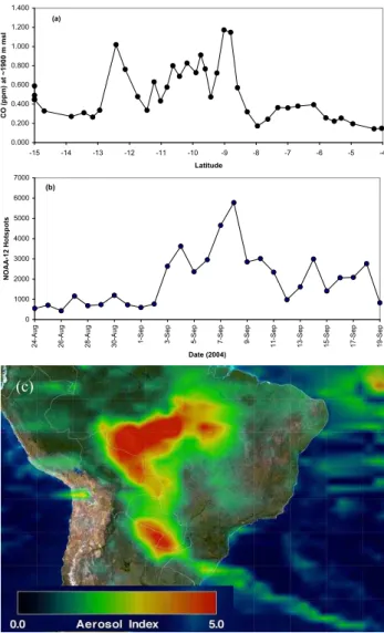
The timing and extent, and perhaps representativeness, of Brazilian biomass burning in 2004 can be compared to other years using metrics other than the regional CO, PM, and O3
values discussed in Sect. 3.2. Dating back to at least 1993 a near-continuous, regional record of aerosol optical thick-ness (Holben et al., 1996; Echalar et al., 1998; http://aeronet. gsfc.nasa.gov/newaeronet1.html) and deforestation rates ex-ists. Unfortunately, the Alta Floresta sun photometer was not operational during the peak of the 2004 burning season
(B. Holben, personal communication). The INPE deforesta-tion data, however, shows 2004 (27 429 km2)as the second highest year after 1995 (29 059 km2)– the year of the SCAR-B campaign. Thus, both TROFFEE and SCAR-SCAR-B were con-ducted in years when the deforested area was well above the long-term average of ∼20 000 km2. The number of NOAA-12 hotspots (http://www.cptec.inpe.br/queimadas/) for 2004 (236 821) is above the 2000–2005 average of 192 569 and just above 2002 (232 921), which was the second-biggest year since 2000. Interestingly, 2002 was the year for another smoke-sampling campaign termed SMOCC (Andreae et al., 2004). While the annual totals for the NOAA-12 hotspots are readily available, they likely underestimate the true num-ber of fires, especially under extreme burning conditions as discussed in Sect. 3.4. In summary, most of our fire sam-pling was probably conducted under “average” conditions as shown in Sect. 3.2, however, the 2004 annual burning was above average because of intense burning beginning ∼7–8 September, which was towards the end of our campaign.
3.3.1 Natural variation in emission factors
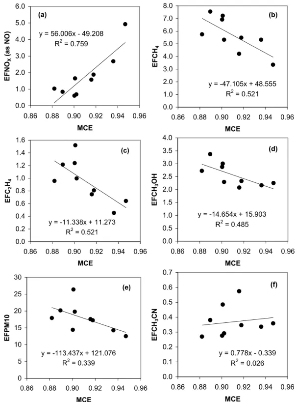
In Fig. 5 we plot the fire-average emission factors versus MCE (data from Table 2) for selected compounds. This gives some idea of the natural variation in emission factors that re-sults from deforestation fires burning under a range of vege-tative/environmental conditions and with different mixtures of flaming and smoldering combustion. Figure 5a shows NOx emissions which increase as MCE (and thus flaming
combustion) increases. Figures 5b–d show the pattern typ-ical of most of the VOC we measured – the EF for these “smoldering compounds” increased with decreasing MCE. Figure 5e shows that EFPM10 also increases with
decreas-ing MCE. The range in EF (with MCE) for these species is about a factor of two, which is a smaller range than we observed for African savanna fires (Yokelson et al., 2003a). Figure 5f shows that EFCH3CN did not have a strong
depen-dence on MCE. This is similar to the pattern observed for HCN from savanna fires by Yokelson et al. (2003a). How-ever, like EFHCN, the EFCH3CN did vary by ∼±50%,
pos-sibly due to varying fuel N content. The use of acetonitrile as a biomass burning indicator/tracer is discussed later in this paper and by Karl et al. (2007a).
3.3.2 Comparison with other work
It is most meaningful to compare our study-average, initial emission-factor measurements in nascent smoke from Brazil-ian deforestation fires with measurements made in August-September of 1990 using a tower-based platform by Ward et al. (1992) during BASE-B; and in August–September of 1995 from an aircraft by Ferek et al. (1998) as part of SCAR-B. We also compare to a widely-used compilation of EF for tropical forests by Andreae and Merlet (2001).
The EFCO2, EFCO, and, especially, MCE all reflect the
overall mix of flaming and smoldering combustion in a fire and thus these parameters can give some idea of the simi-larity of the combustion characteristics of the fires we sam-pled to fires samsam-pled previously. This serves as one probe of how representative our fires were of regional fires in gen-eral. Ward et al. and Ferek et al. report individual values for flaming and smoldering combustion and it is not always clear if they have a recommended study-average for primary forest fuels. However, our study-average MCE for defor-estation fires (Table 2) indicates that they burn with roughly equal amounts of flaming and smoldering (Yokelson et al., 1996). Thus, when necessary, we compare to the average of the flaming and smoldering values given in the other work in the following discussion.
For CO2 the EF are 1614±56 (Ward et al., 1992), 1599
(Ferek et al., 1998), and 1580±90 (Andreae and Merlet). All these values are reasonably close to each other and our study average of 1615±40. Similarly for CO the previous values are 110±28, 105, and 104±20 in excellent agreement with each other and our value of 101±24. The MCE are 0.903±0.03, 0.906, 0.906, and our value of 0.910±0.021. Thus our values are well within the range of previous mea-surements, but seem to reflect slightly more flaming combus-tion on average than previous work.
The research fire on 5 September, which was designed to simulate regional fires apparently had a significantly higher MCE than our regional average. However, the higher MCE partly reflected that we did sample the beginning of the fire, but could not finish sampling the full fire (smoldering con-tributes less at the beginning of a fire) because of aircraft fuel considerations. Our airborne samples showed that MCE ini-tially decreased with time and then stabilized. It is also inter-esting to note that the fires sampled later in TROFFEE tended to have higher MCE, which could be due to the protracted dry period after unusual rains in mid August. Finally, the plume from the intense burning event sampled on 8 Septem-ber (see Sect. 3.4) also had higher than study-average MCE. Thus late-season, “higher-MCE” plumes may account for a fair percentage of the total regional biomass burned. On the other hand, prolonged dry spells will desiccate large diameter logs, which tend to burn with a low MCE (∼0.788, Christian et al., 2007b) producing initially unlofted smoke. So the real nature of the “total regional smoke” is governed by complex – sometimes competing – trends, which need further analy-sis.
Rather than an exhaustive species by species comparison with other work for the numerous other trace gases measured, we have tried to summarize the comparison in Fig. 6 and provide some useful guidance. Then a few comments are made about select individual species. Many compounds ap-pear in both our work (Table 2) and the recommendations of Andreae and Merlet (AM). In general, our values are based on a larger number of measurements and should probably be preferred to those in AM who acknowledge basing many
y = 56.006x - 49.208 R2 = 0.759 0.0 1.0 2.0 3.0 4.0 5.0 6.0 0.86 0.88 0.90 0.92 0.94 0.96 MCE EF N OX (a s N O ) (a) y = -47.105x + 48.555 R2 = 0.521 0.0 1.0 2.0 3.0 4.0 5.0 6.0 7.0 8.0 0.86 0.88 0.90 0.92 0.94 0.96 MCE EF C H4 (b) y = -11.338x + 11.273 R2 = 0.521 0.0 0.2 0.4 0.6 0.8 1.0 1.2 1.4 1.6 0.86 0.88 0.90 0.92 0.94 0.96 MCE EF C2 H4 (c) y = -14.654x + 15.903 R2 = 0.485 0.0 0.5 1.0 1.5 2.0 2.5 3.0 3.5 4.0 0.86 0.88 0.90 0.92 0.94 0.96 MCE EF C H3 O H (d) y = -113.437x + 121.076 R2 = 0.339 0 5 10 15 20 25 30 0.86 0.88 0.90 0.92 0.94 0.96 MCE EF PM1 0 (e) y = 0.778x - 0.339 R2 = 0.026 0.0 0.1 0.2 0.3 0.4 0.5 0.6 0.7 0.86 0.88 0.90 0.92 0.94 0.96 MCE EF C H3 C N (f)
Fig. 5. Fire-average emission factors (EF) plotted versus fire-average modified combustion efficiency (MCE) for the indicated species (data
from Table 2). (See discussion in Sect. 3.3.1).
of their values on 1–2 less direct measurements and/or “best guesses” due to a lack of detailed information available at the time. On the other hand, a number of compounds appear
in the AM recommendations that we did not measure during TROFFEE. Most of these are minor plume constituents, but some are of major importance (e.g. SO2). We recommend
0 0.5 1 1.5 2 2.5 3 3.5 4 4.5 5 CO 2 CO MC E NO x (a s NO ) CH 4 C2H 4 C2H 2 C2H 6 C3H 6 HCH O CH3O H CH 3CO OH HCO OH NH 3 HCN compound formula EF T R O F F EE/ EF A M (a) 0 1 2 3 4 5 6 CH3C N CH3C HO acro lein ace tone prop anal isop rene fura n benze ne 3-me thyl fura n 2-me thyl fura n 2,3 buta nedi one pent anon es tolu ene phen ol othe r su bstit uted Fura ns xylen es ethyl benze ne PM1 0
compound name or formula
EF T R O F F EE/ EF A M (b) 23 18 57 10
Fig. 6. Comparison of the TROFFEE airborne study emission
fac-tors with the recommendations of Andrea and Merlet (2001) (AM) for species in both studies. (AM PM10is taken as 1.3×AM PM2.5.) With 8 exceptions, the older (AM) recommendations are within a factor of ∼2 of the newer TROFFEE EF, which are usually based on more measurements. This suggests that the AM recommendations for species not measured in TROFFEE (e.g. SO2)are reasonable. (a) species measured by AFTIR. (b) species measured by PTR-MS
and the nephelometer. (When the ratio exceeds the scale shown the value of the ratio is given above the bar.)
using the AM values for compounds we did not measure since there is reasonable agreement between our work and theirs on most of the compounds we both address (see Fig. 6). Finally our work includes data on a number of “new,” signif-icant plume constituents for which information was not pre-viously available. Included in this category are HONO, acry-lonitrile, pyrrole, methylvinylketone, methacrolein, croton-aldehyde, methylethylketone, methylpropanal, “acetol plus methylacetate,” furaldehydes, dimethylsulfide, and C1–C4
alkyl nitrates (Table 2).
In early fire research it was usually assumed that most of the NMOC were NMHC as was actually the case for indus-trial combustion of fossil fuels. As mentioned in the in-troduction, a key discovery of previous FTIR and PTR-MS work was that OVOC accounted for the large majority of NMOC emitted by the fires sampled. A goal of this project was to verify this for tropical deforestation fires. The TROF-FEE data show that the molar ratio OVOC/NMHC is about 4:1 – or that OVOC account for ∼80% of the NMOC. With the completion of TROFFEE, there are now reasonably com-prehensive field measurements of the NMOC emitted by all the major types of biomass burning. The new information
provided on the “universal dominance” of OVOC is signifi-cant because of the huge size of the biomass burning source and the reactive nature of OVOC (Mason et al., 2001; Trent-mann et al., 2005).
A few comments are made about individual species we measured. An IR signal due to HONO was observed on the lab fires and 2 field fires, but the measurements are semi-quantitative due to a low SNR. However, the presence of any HONO signal is significant since even a small amount of HONO in the initial emissions is a source of OH that speeds up the initial plume chemistry (Trentmann et al., 2005). Our field, study-average HONO EF (0.26±0.13 g/kg) overlaps the other relevant HONO EF we know of (Keene et al., 2006): 0.24 g/kg shrubs, 0.19±0.08 g/kg branches, and 0.14±0.05 g/kg grass.
As mentioned above, the EF for acetonitrile was not strongly correlated with MCE in our field study. Thus, our study-average EF of 0.37±0.10 g/kg seems to be a good estimate for all tropical deforestation fires regardless of MCE. However, our EF for acetonitrile from deforestation fires does differ significantly from recommended EFCH3CN
for other types of burning (e.g. 0.13 g/kg for savanna fires and 4.91 g/kg for burning Indonesian peat (Christian et al., 2003)). In addition, acetonitrile emissions have not been measured for cooking fires, which may be the second largest type of biomass burning. Still, these results suggest that (with attention to the type of fire) PTR-MS acetonitrile mea-surements could contribute to source apportionment or esti-mates of the amount of biomass burned using inverse model-ing.
The particle emission factors we measured during TROF-FEE (PM10, 17.8±4.1 g/kg) are significantly larger than in
previous work or recommendations. Ferek et al. (1998) re-ported a range of EFPM4from 2–21 g/kg and a study
aver-age of about 11 g/kg for Brazilian deforestation fires. The tower-based measurements of Ward et al. (1992) returned values for EFPM2.5ranging from 6.8 to 10.4 g/kg with an
av-erage of about 9 g/kg for forest fuels. Ferek et al speculated that their higher average and high end values were due to incomplete particle formation being probed from the tower platform. This hypothesis was supported by simultaneous tower and airborne PM measurements on the same Brazilian fires (Babbitt et al., 1996). In that experiment, the airborne EFPM2.5 averaged about 11 g/kg while the EFPM2.5
mea-sured on the same fires from towers averaged about 4 g/kg. In any case our study average value for PM10, which
in-cludes a wider range of particle sizes than the work refer-enced above, is significantly higher at 17.8±4.1 g/kg. For most types of biomass burning the PM10values might be
ex-pected to be about 30% higher than the PM2.5or PM4values
(AM, Ottmar, 2001). Applying this factor to the study aver-age of Ferek et al gives a projected PM10of about 14 g/kg –
still lower than our TROFFEE value. A major reason for the rest of this discrepancy could be related to fire size and inten-sity. Ferek et al. noted that their largest, most intense fire in