CAPACITATED TREES,
CAPACITATED ROUTING, AND
ASSOCIATED POLYHEDRA
by
J. R.
Araque G.,
L. A. Hall and T. L. Magnanti
Capacitated Trees, Capacitated Routing, and Associated Polyhedra
Jesus Rafael Araque G.
CORE
Universit6 Catholique de Louvain
Leslie A. Hall
Department of Civil Engineering and Operations Research
Princeton University
Thomas L. Magnanti
Sloan School of Management
M.I.T.
August 1990
Revised October 1990
Abstract
We study the polyhedral structure of two related core combinatorial problems: the subtree cardinality-constrained minimal spanning tree problem and the identical customer vehicle routing problem. For each of these problems, and for a forest relaxation of the minimal spanning tree problem, we introduce a number of new valid inequalities and specify conditions for ensuring when these inequalities are facets for the associated integer polyhedra. The inequalities are defined by one of several underlying support graphs: (i) a multistar, a "star" with a clique replacing the central vertex; (ii) a clique cluster, a collection of cliques intersecting at a single vertex, or more generally at a central" clique; and (iii) a ladybug, consisting of a multistar as a head and a clique as a body. We also consider packing (generalized subtour elimination) constraints, as well as several variants of our basic inequalities, such as partial multistars, whose satellite vertices need not be connected to all of the central vertices. Our development highlights the relationship between the capacitated tree and capacitated forest polytopes and a so-called path-partitioning polytope, and shows how to use monotone polytopes and a set of simple exchange arguments to prove that valid inequalities are facets.
1
Introduction
The minimal spanning tree problem and the traveling salesman problem are two of the most noted and heavily studied of all combinatorial optimization models. The operations research and applied mathematics communities have devoted enormous energies to developing structural properties and efficient algorithms for solving these problems. In large part, the community's interest in these problems stems from two sources: (i) the problems' inherent attractiveness as mathematical objects, and (ii) the fact that they represent core models both for network design and for a wide variety of routing and scheduling applications.
Although the research community knows much about the structure of the integer programming formula-tions of these problems, it has established surprisingly few results about capacitated versions of these models. Indeed, when we first undertook the research reported in this study, essentially nothing had been reported in the open literature about the polyhedral structure of the capacitated models we are investigating.
Capacitated versions of the minimal spanning tree and the traveling salesman problems have numerous applications as diverse as vehicle routing, facility location, and telecommunication systems planning. For example, a basic problem in telecommunications is the design of a centralized processing network. These networks have one or more central processors that must be linked via a tree topology to several remote terminals which have specified demands that one of the central processors must serve. In practice, the amount of traffic that any link in the network can carry is limited. For the practical situation in which any outgoing link from the central processor can handle only a fixed number of customers, the same for each link, the problem becomes the type of capacitated minimal spanning tree problem that we treat in this paper.
In the past, the research community's ability to solve these capacitated problems by optimization methods (rather than heuristics) has been very limited, in part because the community has not developed a good integer programming representation of the problems. In this paper we address this issue; we undertake a study of the polyhedral structure of two related capacitated versions of these problems: (i) the subtree
cardinality-constrained minimal spanning tree problem (which we also call the K-capacitated minimal spanning tree problem), and (ii) the capacitated identical customer vehicle routing problem. Both of these problems are
deceptively simple to state, but are rather complex mathematically. For the subtree cardinality-constrained minimal spanning tree problem, for a given graph with edge costs, we wish to find a minimum cost tree with the property that no subtree off a designated root vertex contains more than K (a given nonnegative integer)
vertices. (We refer to any tree satisfying this condition as a K-capacitated tree.) For the identical customer vehicle routing problem, we wish to find a minimum cost set of routes, all originating and terminating from a given depot, with the properties that no two routes intersect at any vertex other than the depot, and no route contains more than K customers. Note that if we eliminate the last link of each route, then any feasible set of routes becomes a feasible solution to the subtree cardinality-constrained minimal spanning tree problem. This well known observation, which served as the key idea for Held and Karp's [1970] noted approach to the traveling salesman problem, highlights the intimate connection between these two problems. Therefore, it is not too surprising to discover a close connection between the polyhedral structure of these two problems as well. Indeed, this paper merges and extends two studies that we had independently undertaken: two of us had studied the subtree cardinality-constrained minimal spanning tree problem, and one of us the identical customer vehicle routing problem.
From the perspective of computational complexity theory and from a practical viewpoint as well, both the subtree cardinality-constrained minimal spanning tree problem and the identical customer vehicle routing problem are difficult to solve. Papadimitriou [1978] has shown that the tree problem is strongly NP-hard for values of K between 3 and n/2 (n is the number of vertices in the underlying network); Bienstock [1987], using a reduction from three-dimensional matching, has proven that even the problem of recognizing whether an (incomplete) graph contains a 3-capacitated spanning tree is NP-complete. Since the identical customer vehicle routing problem contains the traveling salesman problem as a special case (when K = n and the edges incident to the depot are sufficiently expensive), this problem is at least as difficult as its notorious TSP cousin. Certain special versions of the problems might be easily solved, however. For example, when
K = 2, both problems reduce to an easily solved nonbipartite matching problem. In this instance it is
possible to give a complete polyhedral description of the underlying integer program (see Hall and Magnanti [1990] for the tree problem).
From an algorithmic perspective, most of the research concerning both the subtree cardinality-constrained minimal spanning tree problem and the (general) vehicle routing problem has focused on heuristic meth-ods. Since several comprehensive surveys describe the state of the art for the vehicle routing problem (for example, see Bodin et al. [1983], Laporte and Nobert [1987], and Magnanti [1981]), we will not review these developments here. We note that although researchers have developed several very clever algorithmic approaches for this, problem class, the exact solution to large-scale problems (for example those with more
than fifty nodes) has remained elusive. Indeed, only recently Fisher [1990] reported solving a 100-customer problem to proven optimality.
The subtree cardinality-constrained minimal spanning tree problem has received much less attention in the literature. Gavish and Altinkemer [1985] have studied approximation algorithms (i.e., heuristics with guarantees on their worst-case behavior) for the version of the problem whose costs satisfy the triangle inequality. Modifying a technique used to study the traveling salesman problem, they devise a (3 - 2/K)-approximation algorithm, that is, an algorithm guaranteed to deliver a tree of cost at most (3 - 2/K) times the cost of the optimal tree. They also give a (4 - 4/K)-approximation algorithm for a general capacitated minimal spanning tree problem in which vertices have arbitrary weights and each subtree off the root vertex has a total vertex weight constraint. Of course by Bienstock's result, no polynomial time approximation algorithm will provide a constant error guarantee for problems with arbitrary costs (i.e., costs that do not satisfy the triangle inequality) unless P = NP (see Garey and Johnson [1979]).
Most of the research on the capacitated spanning tree problem has focused upon developing heuristic procedures that produce feasible solutions; how far these solutions are from optimality is unclear. These heuristic approaches fall into three classes: (i) greedy (merging) algorithms [Esau and Williams 1966, Ker-shenbaum and Chou 1974, Gavish and Altinkemer 1986], (ii) second-order greedy algorithms [Karnaugh 1976, Kershenbaum, Boorstyn and Oppenheim 1980], and (iii) clustering algorithms, for problem defined in the Euclidean plane [McGregor and Shen 1977, Sharma 1983]. Gavish and Altinkemer [1986] present a survey of these three approaches.
Researchers have also attempted to solve the capacitated minimal spanning tree problem by branch and bound [Chandy and Lo 1973, Chandy and Russell 1972, Elias and Ferguson 1974, Kershenbaum and Boorstyn 1983] and by Benders' decomposition [Gavish 1982]. These methods have generally been disappointing: for branch and bound, the solution approach seems limited to problems with at most 20 vertices; Benders' decomposition has been largely unsuccessful, even for problems with from six to twelve vertices.
Gavish [1983,1984] has recently had more success using an augmented Lagrangian based algorithm which generates lower bounds on the value of the optimal capacitated minimum spanning tree. His computational approach is the only work we know that compares heuristic solution values with non-trivial lower bounds. Nevertheless, the gaps between the bounds are still fairly large (on the order of 20 per cent) and point to
the need for a better polyhedral representation of the integer programming formulation of the problem. Bousba and Wolsey [1989] report good computational experience for a related, more general model. The work reported in this paper is motivated by two considerations. First, although recent research has permitted researchers to solve large scale uncapacitated network design problems and uncapacitated network routing problems, capacitated versions of these problems appear to be computationally elusive. For example, Balakrishnan, Magnanti and Wong [1989] have solved to near optimality uncapacitated network design problems with as many as 500 0-1 variables (design arcs) and 2500 commodities, and Padberg and Rinaldi [1989] have solved traveling salesman problems with as many as 2,392 vertices. The subtree cardinality-constrained minimal spanning tree problem and the identical customer vehicle routing problems are, in a sense, the simplest core capacitated network design and network routing models and so insight concerning these models might prove to be valuable in extending the results for uncapacitated problems to more general capacitated models.
Second, mounting evidence in many application domains has demonstrated the impressive potential of using strong cutting plane methods for solving a variety of pure and mixed integer programs (see Hoffman and Padberg [1985] and Wolsey [1989] for surveys). In particular, research on the simpler traveling salesman problem has shown that the type of polyhedral results that we consider in this paper have been very useful, indeed essential, in solving large-scale problems to optimality (with a guarantee of optimality). This expe-rience suggests that a better understanding of the polyhedral structure of capacitated network design and routing problems might lead to effective algorithms. Nevertheless, to the best of our knowledge until now no one has investigated the polyhedral structure of the capacitated minimal spanning tree problem, and only two studies, conducted in parallel with the research we are reporting, have studied the polyhedral structure of the (identical customer) vehicle routing problem. Cornuejols and Harche [1989] have focused on extensions of valid inequalities (for example the well known comb inequalities) for the traveling salesman problem that use routing type structure of these problems. In work not reported here, one of us (Araque [1989b, 1989c]) has also studied these type of inequalities. Cornuejols and Harche [1989] and Campos, Corberan and Mota [1989] have also studied a certain set of extended subtour breaking constraints that we also consider in this paper. In contrast, in this paper we focus on a graph-based approach that does not ensue from natural
In the next section, we introduce formulations for the two problems we are studying as well as a relaxed forest version of the subtree cardinality-constrained minimal spanning tree problem, and a reformulation of the identical customer vehicle routing problem as a certain path-partitioning problem. We also establish relationships between these problems, and particularly between their valid inequalities and facets. These relationships permit us, for the most part, to treat the two problems simultaneously or as modest variants of each other; on some occasions, however, we need to treat the problems differently because the vehicle routing and path-partitioning problems are more constrained than the minimal spanning tree problem (because of the degree-2 constraints of the vertices in a path). Therefore, we introduce some inequalities that are facets for only the path-partitioning polytope.
In this section we also introduce a general proof technique, based upon certain exchange arguments and comparison of certain generic solutions, that permits us to streamline many of our proofs in later sections.
In Section 3 we provide a general introduction of the various types of inequalities we develop in the rest of the paper and some motivating examples to illustrate why the inequalities are needed. Sections 4 through 6 contain technical details for establishing when the inequalities we introduce are valid and facet-inducing. In Section 4 we discuss tree and packing (or generalized subtour elimination) constraints. In Section 5, we consider multisiar subgraphs which are star subgraphs, but with a clique replacing the central node of the star. In Section 6, we consider a certain type of ladybug graph structure and associated inequalities. A ladybug subgraph has two components: a head which is a multistar and a body which is a clique. As we show, under certain circumstances these subgraphs yield facet-inducing inequalities. In this section, we also consider several partial multistar variants of the basic multistar inequalities. In Section 7, we consider a graph structure which we refer to as a clique cluster: it is composed of a set of cliques that meet at a common vertex. Again, we show that certain classes of clique clusters are facet-inducing.
In a concluding section, we suggest possible directions for future research and point out some generaliza-tions of the results reported in this paper.
2
Preliminary Results
2.1
Path Partitioning, Forest, and Tree Polytopes
We begin by introducing notation needed for discussing graph structures. Let G = (V, E) be a complete, undirected graph. For i,j E V, we write ij, ji, or e to represent the undirected edge e = {i, i} E E. For a subset of nodes S C V, we denote the set of all edges between nodes of S by E(S) = {ij : i, j E S}; for any two disjoint subsets S, U C V, we denote the set of edges with one vertex in each of these sets as E(S, U) =
{e = ij : i E S, j E U}. For v E V, we denote the set of edges incident to v as 6(v) = E({v}, V\{v}).
For a set of edges B C E and a vector x = (e, : e E E), we frequently use the notation X(B) =
E
Xe. If eEB f E E, we also let ef denote an incident vector withIEI
components which has value 1 corresponding to the element f of E and value 0 otherwise.Throughout the discussion, we label the nodes of V as 1,... ,n. For the minimal spanning tree problem and the vehicle routing problem, we include an additional special node 0 and define the problems with respect to the complete graph on {0, 1,.. ., n}.
To formulate the subtree cardinality-constrained minimal spanning tree problem as an integer linear program, we introduce some notation. The central root node is the special node 0. We let K denote the subtree capacity, and Ce denote the cost of edge e, for all e E E(V U {O}) = E U {Oj: j = 1,..., n}. The
decision variables,for all e E E(V U {0}), are
1, if edge e is in the tree;
e 0, otherwise. The integer programming formulation is
n Minimize cx + cojzoi
E
eEE j=1 subject to n x, + E Xoj = n (2.1) eEE j=1,
Csl- Xe •sc
v,
sJ>2
(2.2) eEE(S)5E
Xe _< UO-1}, UC, > 2, E U (2.3) eEE(U)Xe E {0, 1}, eE E.
Equality (2.1) is true of all trees. Inequalities (2.3) are some of the rank inequalities for trees: if more than IU[ edges connect the nodes of a subset U, then that set of edges must contain a cycle. Inequalities (2.2) are similar to (2.3), except that they reflect the capacity constraint: if the set S does not contain the root node, then the nodes of S must be contained in is at least [SI1/K] different subtrees off of the root.
Let X be the set of solutions to this integer program. Then we define T to be conv(X), the convex hull of K-capacitated trees.
A closely related problem is the capacitated forest problem. If we delete node 0 and all edges incident to node 0 from a capacitated spanning tree, the resulting graph structure is a forest, each of whose components contains at most K nodes. The following integer program models the problem of finding the minimal capacitated forest on nodes 1,..., n:
Minimize cexe
eEE
subject to
XE
e < ISI-['i
SCV, ISI>2eEE(S)
e E {0, 1), eE E.
If X is the set of solutions to this integer program, then we define F to be conv(X). Section 2.4 explains the relationship between T and F; in particular, we show that any facet of F is a facet of T as well.
Next we turn to a related problem, the identical customer vehicle routing problem. We let K represent truck capacity, cij the cost of traveling between nodes i and j, and, by analogy to the tree problem, we let node 0 be the depot and nodes 1,..., n the customers. The decision variables for our integer programming
formulation are
if i and j are consecutive customers on the same route;
xij = 1
= 0, otherwise, for all i, j E V;
2, if i is alone on a single route;
zi = 1, if i is the first or last customer on a route with at least two customers; 0, otherwise,
for i =1,..., n.
We can then formulate the following integer program to determine the minimum-cost routing: Minimize
E
cede +E
coizieEE i subject to n
z
ij + Zi j=1 = 2,E
, -
K
eEE(S) Xe E {0, 1}, zi E {0, 1, 2},SC V, IS1> 2
eEE i= l,...,n.The variables zi can be treated as slack variables and eliminated from the formulation to yield a new formulation in the x-variables with edge-costs given by the saving sij = coi+ coj - cij as defined by Clarke
and Wright [1964]: Maximize subject to n j=1
E
eEE(S) xijE Se
Xe eEE < 2, e , 1), SCV,ISI>2
e E E.This reformulation of the vehicle routing problem leads to a reinterpretation of the problem in terms of a graph model. A feasible solution to the second integer program, on the node set V = {1,..., n}, consists of
a collection of paths, each containing at most K nodes; we refer to this graph structure as a K-capacitated
path-partition, and to the corresponding optimization problem as the path-partitioning problem. If X is the
set of solutions to the integer program, then we define PP to be conv(X), the convex hull of solutions to the path-partitioning problem.
Observe that any K-capacitated path-partition is a K-capacitated forest, as well. Consequently, PP C F, and any facet of PP that is a valid inequality of F must also be a facet of F. We use this fact frequently in the proofs to follow.
2.2 Exchange Arguments
In proving that certain valid inequalities are facets, we will use the following familiar argument (which amounts to a dual or "indirect" proof).
Suppose that P is a full-dimensional polyhedron in IRm and the inequality ax < ao is a valid face of P (i.e, all points in P satisfy this inequality, and at least one point of P lies on the hyperplane defined by the inequality). Then this inequality is a facet of P if it satisfies the property that if Tx < 'ao for all points x contained in the face Q = {x E P I ax = ao} of P, then (a, ao) is a multiple of (a, ao). One way to establish this result is to identify k > m points x0,..., xk contained in Q with the property that any solution to the
system
CtTX = a0
TX1 = Ot
OtTXk = CO
in the variables (a, a0) is the vector (a, ao) or some multiple of this vector.
We note that the same proof technique applies to situations in which P is not full-dimensional, as is the case for the polyhedron T. If this case, though, we need to show that aTx < ao is a proper face of P-that is, some point of P does not lie on the face defined by this inequality-and that any solution (a, ao) to the previous system is of the form (a, ) = AO(a, a) + P Ai(bi, boi) for some weights A0, )A, ... , Ap with
equations satisfied by all solutions of P. As we show in Section 2.3, for the polyhedron T, the only such equation is X(E(V U {0})) = n.
In many cases, such as the polyhedra defined over graphs that we are considering, it is possible to define the vectors xj two or three at a time to make inferences about some of the coefficients of the vector ca. Since the same elementary constructions recur frequently in our development, to avoid duplicating our arguments and to highlight the ideas we are using, we feel it might be useful to collect and formalize some of these arguments at the outset of our discussion in the form of the following straightforward exchange arguments. Throughout this discussion, P C IRm is an arbitrary polyhedron, and F and PP are the forest and path-partitioning polytopes, respectively. We think of P as being defined on Kn, the complete graph on n vertices.
Lemma 2.1 (Simple-exchange). Suppose x, y E P satisfy aTx = ao and aTy = ao, and that for two given
edges f and g, xf = 1,zg = 0, yf = O, yg = 1 and Xe = Ye for all edges e f f,g. Then the coefficients af and cg are equal.
Proof: Subtract one equation from the other to obtain
afxf - gyg = 0,
or Cf = ag since xf = yg = 1. .
The following two easy extensions of Lemma 2.1 will prove to be extremely useful in streamlining the proofs to follow. Often, a candidate facet has many solutions satisfying it at equality that differ among themselves very little. This structure can be exploited.
Lemma 2.2 (Triple-exchange for forests). Let S be a subset of vertices. Suppose that, for any three distinct
nodes i, j, and k of S, some 0 - 1 vector x in F corresponding to a forest in which i, j, and k are on the same tree satisfies the equality
aTx = a0. (2.4)
Suppose further that we can connect the vertices on the tree containing i,j and k in any way and the incidence vectors of the forests so generated still satisfy (2.4). Then all of the coefficients of E(S) in a are equal.
Proof: Fix x. Without loss of generality, assume that the edges ij and jk are part of the forest. By exchanging edge ik for edge ij and applying the simple-exchange argument, we have aij = arik- Since i, j and k are arbitrary, we immediately conclude that any two edges in E(S) with a common vertex have the same coefficient. Now consider two edges in E(S) with no common vertices, say edges ij and kl. Using the
triplets i, j, k and j, k, 1, we obtain cij = acjk = akl* ·
Lemma 2.3 (Triple-exchange for paths). Let S be a subset of vertices. Suppose that, for any three distinct
nodes i, j, and k of S, some 0 - 1 vector x in PP satisfies the equality
a Tx = ao, (2.5)
and the path-partition corresponding to x contains a path of the form k - j - i - , with k as an endpoint. Suppose, further, that if we permute the vertices in this path, we obtain another vector satisfying (2.5). Then all of the coefficients of E(S) in oe are equal.
Proof: First, let x correspond to a partition containing the path k - j - i - , and let y be obtained
from x by permuting nodes k and j so that the resulting partition contains the path j - k - i - .. From
the simple-exchange lemma applied to x and y, we obtain caik = aij. The result now follows by the same arguments given in the proof of Lemma 2.2.
Lemma 2.4 (In-and-Out edges). Suppose x E P satisfies aTx = ao, and that xf = 0 for a given edge f. If
it is possible to switch the edge f in and out of the solution and remain on the face aTx = ao (i.e., if we can change xj to 1 and still obtain a vector in P satisfying the equation aTx = ao), then Cf = 0.
Proof: Subtracting the equation aTx = (o from aT(x + ef) = ao yields af = 0. Of course, Lemmas 2.1, 2.2, and 2.4 apply to the polytope T as well.
2.3 Dimensions of PP, F, and T
The dimension of a polyhedron P is defined as the dimension of the smallest affine space containing P. In general, facet proofs are easier for full-dimensional polyhedra than for lower-dimensional ones. As shown by the following lemma, both F and PP are full-dimensional. Let m = n(n - 1)/2.
Lemma 2.5 Dim F = dim PP = m.
Proof: Since PP C F C IRm, it suffices to show that dim PP = m. To do so, we need simply to exhibit a set of m + 1 affinely independent vectors contained in PP. The O-vector along with the unit vectors el, ... , em comprise such a set (ei contains a 1 in the i-th component and a 0 elsewhere). e
The polytope T does not have full dimension, since every tree satisfies
X(E(V U {O})) = n. (2.6)
Lemma 2.6 Dim T = (n + 1)n/2 - 1.
Proof: Recall that T C IR(" + l )n/ 2 . To prove the lemma, it is sufficient to show that (2.6) is the only equality (up to a multiplicative factor) containing T. Consider an arbitrary equality
ax = ao (2.7)
containing T, and consider the star-shaped tree consisting of all of the edges incident to the root, or y =
(Yoi = 1, i = 1... ,n; Ye = 0, e E E). Clearly y satisfies (2.7). Now consider two arbitrary nodes i,j 0,
and replace edge Oi or Oj in y by edge ij. Since these new solutions also satisfy (2.7), by the simple-exchange argument (Lemma 2.1) we have
0oi = aOj = aCij (2.8)
Since i and j were arbitrary, all of the edges incident to the root have the same coefficient in (2.7); and thus by (2.8), all of the edges do. Thus (2.7) is indeed a multiple of (2.6).
2.4 Extending facets from F to T
The following lemma emphasizes the close relationship between F and T. It states that any facet for F can be trivially lifted to T.
Proof: Let aTx < ao be a facet for F such that ao > 0. (Note that ao 1t 0, since the O-vector is valid for aTx < ao.) Since F is a full-dimensional polytope in IRm, it contains m linearly independent 0-1 vectors xl,... x, E IRm satisfying aTx = ao. We can arrange these vectors as rows of a matrix X, and their linear independence implies that the matrix is invertible. Each vector xi is the incidence vector of a forest with n vertices. By adding edges to connect each component of the forest to the root vertex, we can obtain vectors in T of the form xi = (xi, yi) with yi corresponding to the vector of edges incident to the root.
Now, let us assume that
?TX + iTy < YO (2.9)
defines a facet of T containing the face defined by aTx = a; that is, every solution (z, y) of T satisfying
aTx = a also satisfies 2.9. We need to show that for some scalars 7 > 0 and p, 7 = ira+pl and Pf = pl (in the first equality 1 is the m-dimensional vector of all ones, and in the second equality it is an n-dimensional vector).
First, we establish
fi = p1. Since the face aTx = a is non-trivial, for each i, j < n it contains a feasible
vector xl for some 1 < I < m with a 1 in the component corresponding to the edge ij. We can extend this vector to a vector in T so that i is connected to the root. By exchanging that edge with the edge connectingj and the root, by the simple-exchange argument (Lemma 2.1) we can show that the coefficients in (2.9) of
edges Oi and Oj are equal; and since i and j were chosen arbitrarily, we see that all of the edges incident to the root have the same coefficients in (2.9). Thus 8f = p1, for some scalar p.
Next we show that y = Ia + p1 for some scalar 7r. If the vector xi defines a forest with ci components, then 1Txi = n - ci and so (here, 1 is a vector of m ones)
m
X1 = Z(n-ci)ei, and (2.10)
i=l
Xa = a01. (2.11)
Since i = (xi, yi) satisfies (2.9) at equality, we have
TXi +- Tyi = yTXi + Ci = o0,
which yields the system
m
X = 01 - p iei.
Since X is invertible, we can solve for y and use (2.11) to obtain
m m
= X-o101 - X- 1' ,ciei = a -X- ' Icie.
i=1 aO iao
Substituting from (2.10), rearranging, and applying (2.11) yields
' =- a -X-- -1
(
cie. nl +nl ao 70 - X-'(-pXl) - X- 1pnl a0 = 'Ya+/ - /na ao ao70
- /n -- a +/al. a0Taking qr = (yo - pn)/ao establishes the relationship.
Finally, we observe that rl > 0. Since (2.9) defines a facet of T, we have yo - pn
$
0. It is easy to verify that this quantity is strictly positive by substituting the incidence vector of the tree with every node connected directly to the root in (2.9), yielding an < 7o. Since a > 0, we have 77 > 0. e2.5
Trivial Inequalities
Finally, we establish that, in general, the trivial inequalities xe > 0 and xe < 1 are facets.
Proposition 2.8 For the polytopes PP, F, and T, if K > 2 and n > 2 the inequalities
Xz > 0 (2.12)
are facets, for all e E E; and if K > 3 and n > 2, the inequalities
Xe < 1 (2.13)
are facets, for all e E E.
Proof: Clearly these inequalities are valid for PP. Suppose that ax < coo is a facet for PP satisfied at equality by every feasible solution satisfying (2.13) at equality, for some edge e E E. Consider the particular solution containing only the edge e. Since for I > 3 a solution containing e and exactly one other edge f also satisfies (2.13) at equality and is feasible for PP, by Lemma 2.4 (the in-and-out argument) crf = 0 for
all f e. This conclusion is sufficient to show that ax < ao is a multiple of (2.13), and thus (2.13) is a facet of PP.
The argument for (2.12) is completely analogous. Since (2.12) and (2.13) are valid for F, they are facets of F, as well; and by Lemma 2.7, (2.13) are also facets of T.
We observe that when K = 2, inequalities (2.13) are not facets for any of the polytopes (unless n = 2), since they are dominated by the valid inequalities xij + Xjk + Xik < 1 on any three nodes i, j, and k.
Proposition 2.9 For K > 2 and n > 2, the inequalities
xoi < 1 (2.14)
are facets for T; and for K > 3 and n > 3, the inequalities
xoi > 0 (2.15)
are facets for T.
Proof: First, we observe that (2.14) and (2.15) are valid for T, and that there are solutions satisfying these inequalities as a strict inequality. Let ax < a0 be a facet of T satisfied at equality by every feasible solution satisfying (2.14) at equality for some fixed i E V. We need to show that this facet is a linear combination of (2.6) and (2.14). In particular, the star-solution x = (oj = 1, j = 1,...,n; Ze = 0, e E E) satisfies
(2.14) at equality. By substituting edge jk for Oj in x, for j 0 i, using the simple-exchange lemma we see that aoj = cjk for all j i, k = 1,..., n; and by the same argument as that in Lemma 2.6, ae = af for all e, f
#
Oi. Thus ax = a0o is a linear combination of (2.14) and (2.6).Similar arguments establish that the inequalities (2.15) are facets under the given conditions. *
When K = 2, the inequalities (2.15) are not facets. Certain facets described in Sections 4 and 5 dominate these inequalities. For example, the inequality X(E(S)) < IS- 1, for S = (VU{0})\{i}, described in Section 4, dominates (2.15) if K = 2.
3
Facets for the Forest, Tree and Path-partitioning Polytopes:
an Introduction
In the following sections, we discuss a number of different inequalities and facets for the forest, tree, and path-partitioning polytopes. Since the description of these inequalities, the associated facet proofs, and the conditions for ensuring that the inequalities are facets are fairly delicate, our discussion is necessarily quite detailed. Therefore, before launching into this development, in this section we will first provide a brief preview of these results, introducing some of the various inequalities and providing some examples to demonstrate their value in cutting off fractional solutions from the linear programming relaxation of the problems. We hope that this more introductory and informal discussion will provide some useful motivation for the remainder of this paper as well as some insight concerning the nature of the various polytopes.
Consider any valid inequality
aex ao eEE(N)
for one of the polytopes that we are considering. We will refer to the subgraph of the original network (V, E) spanned by those edges e with ae
#
0 as the support graph of this inequality. Since essentially all of the inequalities that we will be considering have a natural interpretation in terms of their associated support graphs, as we introduce the various inequalities we will describe their support graphs, illustrate feasible solu-tions on the support graphs, and identify fractional solusolu-tions from one of the linear programming relaxasolu-tions LPF, LPT and LPP P that the inequality cuts off. In most cases, if we make appropriate restrictions on the problem data and the configuration of the support graph, the inequalities will be facets for all of the polytopes F, T, and/or PP; we will draw our examples from the most restrictive of these polytopes, that is, from PP.We will introduce four types of inequalities:
(1) multistars (large and small), (2) partial multistars,
(3) ladybugs, and (4) clique clusters.
C
-N. ½~
& N
*A~
~
(a) Support graph
(b) Feasible solution
-.01P
\ \-, : . Ile-, ... "q% .. I . .... N....\
'%4
.: B
;~ '.. -~
r;l',.Weight
1/2
Weight 1/2
Weight 1
(c) Feasible solution
(d) Fractional solution cut away
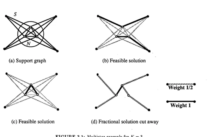
FIGURE 3.1: Multistar example for K = 3
Within in each type, we will describe several variants. For example for the multistars, we describe both "large" and "small" multistars.
Multistars
The support graph of a basic multistar looks like a simple star graph except that a clique replaces the central vertex of the star. That is, a multistar consists of the complete subgraph on a set of nucleus vertices
N, together with a set of satellite vertices S and the edges connecting every satellite vertex to every nucleus
vertex. The support graph for the example shown in Figure 3.1 has four satellite vertices and a three-vertex nucleus. As shown in Figures 3.lb and 3.1c, since K = 3 for this example, any feasible solution to the path-partitioning problem can contain at most four edges from the support graph of this multistar. Moreover, note that if we assign a weight of K = 3 to the edges in the nucleus of the multistar with and a weight of one to those edges joining the nucleus vertices and the satellite vertices, then the total weight of the support graph of the multistar in any feasible solution to the path-partitioning polytope is at most six. Therefore, we can write the valid inequality
Note that the fractional solution shown in Figure 3.1d violates this inequality; it has a total weight of 6 1/2. We might note that this particular fractional solution is an extreme point of the packing path-partitioning polytope, that is, the linear programming formulation of the problem with all of the degree-2 constraints, the packing constraints (2.2), and the trivial inequalities (2.12) and (2.13).
In general, the multistar inequality is of the form
KX(E(N)) + X(E(N, S)) < (K - 1)INI.
If we impose certain conditions on the sizes of the nucleus and satellite sets, and if these two sets contain all the vertices V of the underlying network, then this type of large multistar inequality is a facet of each of the polytopes F, T, and PP (the conditions required for the polytope PP are more restrictive than those for the forest and tree polytopes). There is, however, another set of facets, which we refer to as small multistars, whose vertex set need not exhaust all of the vertices V of the original network. In this case the coefficient b of the nucleus edges is less than K and the right-hand side of the inequality is less than (K - 1)INI. That is, the inequality is of the form
bX(E(N)) + X (E(N, S)) < RS.
This small multistar is a facet of each of the three polytopes for certain choices of the constants b and RHS if we impose appropriate restrictions on the relationships between the sizes of the nucleus and satellite sets (see Section 5).
Partial Multistars
For the path-partitioning polytope, we can also generalize the multistars in another way. Instead of including all the edges connecting the nucleus vertices and the satellite vertices, the support graph contains only those edges that are incident to a subset N of the nucleus vertices; we refer to this subset as the
connector vertices. In Section 6 we will develop facet versions of these inequalities with one, two, and three
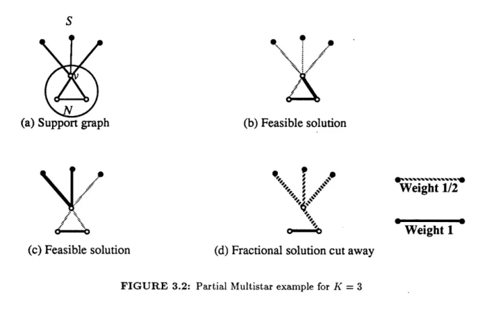
connector vertices. Figure 3.2 shows the support graph of a partial multistar with one connector vertex v, as well as feasible solutions, and a fractional solution that we wish to cut away. As shown in Figures 3.2b and 3.2c, the support graph for this partial multistar can contain at most three edges in the induced subgraph corresponding to any feasible solution to the path-partitioning problem. Moreover, note that the nucleus set can contain at most two of these edges, and that if a feasible solution uses two of these edges then it cannot use any edge to a satellite vertex. Consequently, if we assign weights of two to the edges joining vertices in
S
(a)
(b) Feasible solution
Weight 1/2
Weieht 1
- -,a--.(c) Feasible solution
(d) Fractional solution cut away
FIGURE 3.2: Partial Multistar example for K = 3
the nucleus set and assign a weight of one to the edges joining the connector vertex v to the satellite nodes, then the total weight of the edges in the partial multistar can be no more than four. Therefore, we can write the following valid inequality
2X(E(N)) + X(E(v, S)) 4
which cuts away the fractional solution in Figure 3.2d. In general, if N is the connector set, INI < 3, we can write a partial multistar inequality of the form
aX(E(N)) + X(E(N,S)) < RHS
and for an appropriate choice of the coefficients a and RHS, and appropriate size restrictions on the size of
N and S, this inequality defines a facet of the path-partitioning polytope. Section 6 describes the details
and also introduces another related facet defined on the same support graph as the partial multistar.
Ladybugs
A ladybug has a support graph with two components: its head is a multistar (N, S), and its body is the complete subgraph on another set of vertices, B, all of which are connected to every vertex in the nucleus set N of the multistar. In this instance, we might interpret the edges connecting the satellite vertices S to
S
(a) Support graph
(c) Feasible solution
(b) Feasible solution
(d) Feasible solution
0Weight 1/2
Weight 1
(e) Feasible solution
(f) Fractional solution cut away
FIGURE 3.3: Ladybug example for K = 3
the nucleus set N as the set of antennae of the ladybug. Figure 3.3 gives a 8-vertex example of a ladybug, together with the induced subgraphs corresponding to feasible solutions to the path-partitioning polytope, and a fractional solution to be cut off by the ladybug inequality. In this example, the head has six vertices: four are satellite vertices and two are in the nucleus. The body of this ladybug has two vertices. In this case K = 3. Note from Figures 3.3b-3.3e that the support graph induced by any feasible solution to the path-partitioning polytope contains at most five edges. Moreover, note that if we weight the edges joining the nucleus nodes with a weight of three, the edges incident to the body vertices with a weight of two, and the edges joining the nucleus vertices and the satellite vertices with a weight of one, then the overall weight of any solution is at most six. Therefore., we can write the valid inequality
(b) Feasible solution
,~t
.S7
Weight1/4
_t
am, v *X ~p4~~ ' W;"t VT ir11 X(c) Feasible solution
(d) Fractional solution cut away
FIGURE 3.4: Clique cluster example for K = 5Note that the fractional solution given in Figure 3.3f does not satisfy this inequality. This fractional solution does satisfy all of the degree-2 constraints, all the subtour elimination (packing) constraints, and all of the large and small multistar constraints. In fact, it is possible to show that it is an extreme'point of the linear programming problem defined by these constraints.
In general, the ladybug constraints have the form
dX(E(B)) + dX(E(B, N)) + KX(E(N)) + X(E(N, S)) < RHS
for some appropriate choice of the coefficient d and of the right-hand side coefficient RHS. In Section 6 we specify the values of these coefficients as a function of the problem data and show when the ladybug inequalities define facets.
Clique clusters
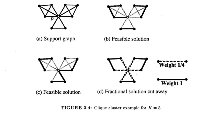
The support graph of a basic clique cluster looks somewhat like a flower and captures some of the properties of cliques and of a cutset around a single vertex. As shown in Figure 3.4, a clique cluster is a collection of subsets of vertices C1, C2,. .. , Ct, each inducing a subgraph that forms one of the cliques or petals of the cluster. The clusters intersect at a single central vertex p, which we will refer to as the
nucleus of the cluster. The support graph for the example shown in Figure 3.4 has three petals, defined by
two cliques with four vertices and one clique with three vertices. As shown in Figures 3.4b and 3.4c, since
(a) Support graph
K = 5 for this example, and because the petals of the clique cluster all intersect at the nucleus vertex, any
feasible path-partitioning solution can contain at most 6 edges from the support graph of this clique cluster. Therefore, we can write the valid inequality
X(E(C1)) + X(E(C2)) + X(E(C3)) < 6.
Note that the packing (subtour elimination) inequalities would require that this sum be less than only 9 - [9/5] = 7. So the clique cluster inequality is stronger when applied to this subgraph. Figure 3.4d shows an example of a fractional solution that satisfies all of the packing inequalities, but not the clique cluster inequality. In general the clique cluster inequality is of the form
ZX(E(Cj)) < RHS, j=1
the right-hand side coefficient RHS being defined by the structure of the clique cluster and the value of K (see Section 7).
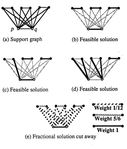
One natural generalization of the clique cluster would be to replace the nucleus vertex by a more general graph. Figure 3.5 gives an example with K = 3 in which the nucleus contains two vertices p and q, each of the cliques in the clique cluster has four vertices, and the cliques have the nucleus as their common intersection. As shown in Figure 3.5b-3.5d, the number of edges in the support graph of any feasible solution can be at most five. But also note that if we weight the nucleus edge pq with a weight of two and every other edge with a weight of one, then the total weight of the edges from the clique cluster in any feasible solution can be no more than five. The fractional solution shown in Figure 3.5e violates this inequality, even though it satisfies all of the packing inequalities as well as all of the clique-cluster inequalities with a single-vertex nucleus. If we let C1, C2, C3 denote the three 4-vertex petal cliques (including the nucleus nodes p and q)
shown in Figure 3.5 let C = C1 U C2 U C3 - N, and let N = {p, q} denote the nucleus, then this extended
clique cluster inequality becomes
X(E(C1 - N)) + X(E(C2- N)) + X(E(C3 - N)) + X(E(N, C)) + 2X(E(N)) < 5.
In general, if C = C1 U C2 U -. U Ct - N, the extended clique cluster inequality has the form t
E X(E(Cj - N)) + X(E(N, C)) + bX(E(N)) < RHS. (3.1)
j=1
The coefficient b < K and the right-hand side RIIS are again determined by the structure of the clique cluster and the capacity K (see Section 7).
\.. . .\ .
\,,
A4i,·6 P*\·~:~xi ?>
~
p '·5·~(a) Support graph
(b) Feasible solution
:-e .. -....
'.
, ,\ I:4
(c) Feasible solution
(d) Feasible solution
- - - - - -
-Weight 1/12
Weight 5/6
Weight 1
(e) Fractional solution cut away
FIGURE 3.5: A generalization of a Clique Cluster for K = 3
Notice that for this general form, we can view the ladybugs as special cases of clique clusters for which the clique cluster nucleus is the ladybug head nucleus, and the petals are the nucleus plus a single node and the nucleus plus the body. Viewed as a clique cluster, the ladybug has a more complicated coefficient structure than that given by 3.1. At the end of Section 7, we discuss this very general structure, which can be viewed as subsuming all of our inequalities, and we indicate the combinatorial problems associated with determining what coefficients are needed to construct facets.
4
Packing or Generalized Subtour Elimination Constraints
We begin with a class of valid inequalities that appears in the integer programming formulation of the polytopes PP, F, and T.
Proposition 4.1 Let N C V with either
(i) INI mod K $ 0, K > 2, (ii) N = V, K >3.
Then the packing inequality
X(E(N))
< INI
-[K
l
(4.1)defines a facet of the polytopes PP, F, and T.
Proof (Validity): A simple packing argument establishes the validity of (4.1). Since the capacity constraints imply that the nodes of N must be partitioned into at least [lNI/K] components, any solution of PP, F, or
T contains at most INI - rlNI/K1 edges of E(N).
(Facet): We shall prove that (4.1) is a facet of PP, and by Lemma 2.7 and PP C F, we shall have proved that (4.1) is a facet for all three polytopes. Let INI = aK + b, 1 < b < K - 1, or b = K and N = V.
We refer to the generic solutions A, B, and C in Figure 4.1, each of which contains a paths with K nodes apiece and one path with b nodes. Since any edge ij with i, j V N can be in or out of a solution satisfying (4.1) at equality, by Lemma 2.4 aij = 0 for these edges.
Next for problems that satisfy condition (i), we consider edge uv in the solution in Figure 4.1A. Since edge uv is an in-and-out edge, auc = 0; and since u and v are arbitrary nodes of N and V\N, respectively, we have aij = 0 for all edges ij in the cutset E(N, V\N). (If V\N is empty, as in condition (ii), then this argument is unnecessary.)
It remains to show that all coefficients of edges in E(N) are equal. For K > 3, by the triple-exchange argument (Lemma 2.3) this result is immediate. For condition (i) and K = 2, the simple-exchange argument (Lemma 2.1) applied to Figure 4.1B implies that au, = au,, and applied to Figure 4.1C implies that auw = c wj, SO that au, = awj. Since u, v, w, and j were chosen arbitrarily, we have the result.
N
L '1' F~~~o~
_ ,(A)
(B)
N(C)
FIGURE 4.1: Generic solutions for the packing facets
A set of inequalities closely related to the packing inequalities are the tree inequalities (2.3) for T. By arguments very similar to those just given, we can prove the following (see Hall [1989]):
Proposition 4.2 Let N C V U {O}, with node 0 E N and N 0 V. Then the tree inequality X(E(N)) < NI- 1
is a facet of T.
We observe that these inequalities correspond to those for the unconstrained minimum spanning tree. Only those inequalities containing node 0 are facets, however, since otherwise the inequalities are dominated by the inequalities (4.1).
5
Multistar Inequalities
In this section we describe those multistars that define facets of the polytopes F, T and PP. First, we introduce two different types of multistars that define facets of F and T:
(i) "large" multistars with vertex set N U S = V (see Proposition 5.1), and
(ii) "small" multistars whose vertex set N U S might be smaller than V, but that are facets only when we impose some tight conditions relating INI and ISI (see Proposition 5.2).
To prove that both types of multistars define facets, we identify some generic solutions and use the exchange arguments introduced in Section 2.
Because the polytope PP is defined by a more tightly constrained version of the integer programming formulation defining the polytope F, since it contains the degree-2 constraints, we might expect that some of the multistar inequalities that are facets for F become lower dimensional faces for PP. Therefore, we might expect the pool of facet-inducing multistars for PP to be smaller than those for F, as reflected by the extra requirements that need to be imposed on the problem data. Propositions 5.3 and 5.4 identify the conditions that we require in the case of the polytope PP for the large and small multistars described in Propositions 5.1 and 5.2. The proofs are somewhat different because the generic solutions we use must satisfy the degree-2 constraints. In addition, the introduction of the degree-2 constraints produces a new set of multistar inequalities which are facets of PP and that we describe in Proposition 5.5. Like the large multistars, they have N U S = V but the described resulting inequalities have smaller coefficients. And unlike the multistars described in Propositions 5.3 and 5.4, most of those described in Proposition 5.5 do not yield valid inequalities for the polytope F. The exceptional case is described at the end of the section.
For each of the inequalities we have considered, we have attempted to give the best possible set of conditions under which they define facets. Relaxing the conditions imposed by our hypotheses would either cause the inequalities to become invalid, or reduce the dimension of the faces they define so that they are no longer are facets.
5.1
Forest and Tree Polytopes
Proposition 5.1 (Large multistars) Let K > 3 and let M be a multistar with a nucleus set N and a satellite
set S satisfying either of the following two sets of conditions:
(i) NI = aK + b, 1 < b < K - 1, a, b nonnegative integers, S = V - N and ISI > 2K - b.
.(ii) INI = aK, a a positive integer, S = V - N and Sl > K + 1. Then the multistar inequality
KX(E(N)) + X(E(N,S)) < (K - 1)IN (5.1)
defines a facet of the polytopes F and T.
Proof (Validity): We give a simple packing argument to establish the validity of (5:1). Let x be any solution maximizing the left-hand side of (5.1) over F, and which has 0 coefficients corresponding to the edges not in the support graph of the inequality. Note that this solution corresponds in a natural way to a bin packing of all the vertices in N and a few of the vertices in S. Suppose that the bin packing has c bins each with a capacity of at most K vertices, that every bin contains at least one vertex in N, and that vertices in different bins are not connected directly by an edge in the solution x. Because the edges in E(N) have a larger coefficient in (5.1) than do the edges in E(N, S), all the nucleus vertices in the same bin constitute a connected subgraph. Since there are c of those components (i.e. bins) with a total capacity of cK vertices, the bins contain at most cK - INI spaces for the vertices in S. We tie these vertices to the nucleus using edges in E(N, S), each with a coefficient of 1 in (5.1). The left-hand side of (5.1) becomes
K(INI - c) + (cK - INI) = (K - 1)INI.
(Facet): We will refer to the generic solutions A to E in Figure 5.1.
The vertices inside each of the ovals are part of the nucleus. The number of free satellite vertices in the solutions A, B and C corresponds to the lower bound on S imposed by the conditions in (i) and (ii). As
at least
K+1
S 0(A)
at least K
_ _-- % K-b
(C)
K-I
K-b
(E)
FIGURE 5.1: Generic solutions for the multistar facet (5.1)
free satellites
K-1
free satellites
K-i
o
free satellites
* *K-1
FIGURE 5.2: ExchangesK-i
at least
1
(B)
2K-b
(D)
* * .mentioned in Section 2, we assume that aTx < ao defines a facet of F containing all the points that satisfy (5.1) as an equality. We consider three different values for the cardinality of N, namely INI =
aK, INI = aK + 1 and INI = aK + b for 2 < b < K - 1.
For INI = aK we consider only the generic solutions A and B. Since we can regard any edge with both
endpoints in S as an in-and-out edge in the generic solution A, oij = 0 for i,j E S. Now consider the component of the generic solution B containing K - 1 vertices from N and one vertex from S. Exchange the edge in solution B connecting the single satellite vertex to the nucleus vertex with any other edge connecting a free satellite to any nucleus vertex in the same component, as in Figure 5.2 because we are free to choose the satellite vertex and the vertex in the nucleus arbitrarily, the simple-exchange argument (Lemma 2.1) implies that aij = A for i E N, j E S for some constant A. By subtracting the equations corresponding to the generic solutions A and B, we immediately have aij = KA for i, j E N and so
aTx = A(KX(E(N)) + X(E(N, S))). This result shows that the multistar inequality (5.1) is a facet when INI = aK.
For the remaining two cases we use the other three generic solutions. We can consider any edge joining two of the (at least K) free satellite vertices in the generic solution C as an in-and-out edge, and so aij = 0 for both i,j E S. Since K - b > 1 the solution C contains at least one edge e* from E(N, S). We can exchange this edge for any edge connecting the same nucleus vertex with any one of the free satellite vertices. The simple-exchange argument proves that aij = Ai for i E N and j E S, i.e., the coefficient is independent of j.
Now, we distinguish between the two cases. If INI = aK + b for 2 < b < K- 1, then we can exchange the
edge e* for an edge joining a different nucleus vertex in the same component (which exists since b > 2) and the same satellite vertex. The simple-exchange argument shows that Ai = A for i E N. By subtracting the equations corresponding to the generic solutions C and D (note that the generic solution D does not exist if b = 1), we see that acij = KA for i,j E N so that arTx = A(KX(E(N)) + X(E(N, S))) and the multistar
inequality (5.1) is a facet when INI = aK + b for 2 < b < K - 1.
If INI = aK + 1 and a = 0, our prior results already show that the inequality aTx < ao is a scalar multiple of (5.1). If INI = aK + 1 and a > 1, we must use the generic solution E to show that Ai = A for i E N. We apply a simple-exchange argument using the component containing K - 1'nucleus vertices and
in Figure 5.2. This exchange shows that Ai = A for i E N. By subtracting the generic solutions C and E, we see that atij = KA for i, j E N and consequently that the inequality etTx < cao is again a scalar multiple of
(5.1). The result for the polytope T follows from Lemma ??. a
Proposition 5.2 (Small multistars) Let K > 3 and let M be a multistar with a nucleus set N and a satellite
set S satisfying both of the following conditions:
(i) INI + IS = aK + b, 1 < a, 2 < b < K - 1, a,b nonnegative integers,
(ii) b < IS < (K-1)INI.
Then the multistar inequality
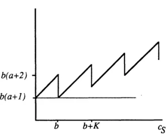
bX(E(N)) + X(E(N,S)) < b(lNI - a - 1) + ISI (5.2)
defines a facet of the polytopes F and T.
Proof (Validity): Let x be any solution maximizing the left-hand side of (5.2) over F, and which has zero coefficients corresponding to the edges not in the support graph of the inequality. Then, the support graph of x corresponds to a forest. Because of the special structure of that support graph, every tree in this forest has either vertices in N and S, or vertices in N only, or is a single vertex in S. Since the inequality coefficients for the edges in E(N) in (5.2) are larger than those for the edges in E(N,S), all the nucleus vertices in the same component must be joined together, i.e., if we remove the satellite vertices, the nucleus vertices in the same component of the forest still induce a connected subgraph. Let CN be the number of trees containing a nucleus vertex, and let cs be the number of trees that are isolated satellites. Then, the left-hand side of (5.2) becomes
b(INI- CN) +
ISI-
cs. Maximizing this expression is equivalent to minimizing bCN + cs. Now,bcN +cs > b [INI + - c = aK + b - cs+cs = ab+ b[b c]+cs.
K K K
Consider the last term as a function of cs. Note that it has value b(a + 1) for cs = O, then it increases
b(a+2)
b(a+l)
FIGURE 5.3: Function ab + b [b Rcs1 + cS
of b units occurs after cs has increased by K additional units, and the value of this function continues to increase by K units and then fall by b units (see Figure 5.3). Consequently the function has only two minima for nonnegative values of cs. Therefore, the left-hand side in (5.2) is at most bINI + ISI -b(a + 1), proving
the validity of the inequality.
(Facet): We break the proof into three different subcases. We obtain these cases by looking at how SI decomposes modulus (K - 1), and then considering the possible values for INI that are consistent with the restrictions imposed by (i) and (ii).
(CASE 1) ISI = t, b < t < K -1, INI = (K-t) + b+ uK; (CASE 2)
IsI = s(K - 1) + t,
1 < s, 1 < t < K - 2, INI = s+(b-t), 1 < b - t < K-2; (CASE 3) ISI = s(K - 1) + t, 1 < s, 1 < t < K- 1, INI = s + (K -t) +b+ uK.In the first case a = u + 1, in the second a = s, and in the third a = s + u + 1. In the remainder of the proof, we refer to the generic solutions Al, B1, A2, B2, A3, and B3 shown in Figure 5.4. The numerical reference corresponds to one of the three cases we have identified above. We eliminate the numerical reference (i.e., refer to A instead of Al, A2 or A3) when the argument applies to all three cases.
t
b
I ;(B1)
b
K-1
/
-(A2)
(B2)
K-i
K-b
b-i
t
(A3)
K-i
K-b-
b
(B3)
FIGURE 5.4: Generic solutions for the multistar facet (5.2)
t


![TABLE I Parameter choices for the generic solutions Generic s t u Solution A LK-1_bj L 2 -ba 1 + K-'b] 2 [K1-b 2 - K-b 2 _ B L 2 K-bJ [2K-b] - [2K-bj a + 2- 2K-b 1 C 0 0 a D (K > 5) [LJ _K- L§J a + 1-[ ] D (K = 4](https://thumb-eu.123doks.com/thumbv2/123doknet/14197449.479337/39.924.150.770.133.918/table-parameter-choices-generic-solutions-generic-solution-lk.webp)
