Characterization of unsteady loading due to impeller-diffuser interaction in centrifugal compressors

Characterization of Unsteady Loading Due to

Impeller-Diffuser Interaction in Centrifugal

Compressors

MA SSACHUSETTS _{INST TU}

by OF TECHNOLOGY

Christopher Lusardi

r JUN 13 2012

B.S., University of Missouri (2009)

_LIBRARIES

Submitted to the School of Engineering

_ARCHNES

in partial fulfillment of the requirements for the degree of

Master of Science in Computation for Design and Optimization

at the

MASSACHUSETTS INSTITUTE OF TECHNOLOGY

June 2012

@

Massachusetts Institute of Technology 2012. All rights reserved.

Author ...

f-I

/

Certified by ...

Senior Research Engineer,

I?

Certified by....

School of Engineering

April 26, 2012

Choon S. Tan

Gas Turbine Laboratory

Thesis Supervisor

... /'... .

6..

.

_{K aren W illcox}

Associate Professor of Aeronautics and Astronautics

(-m--,CDO Reader

Accepted by ...

Nic . adjiconstantinou

Associate Professor of /Jechanical Engineering

Director, Computation for Design and Optimization

Characterization of Unsteady Loading Due to

Impeller-Diffuser Interaction in Centrifugal Compressors

by

Christopher Lusardi

Submitted to the School of Engineering

on April 26, 2012, in partial fulfillment of the requirements for the degree of Master of Science in Computation for Design and Optimization

Abstract

Time dependent simulations are used to characterize the unsteady impeller blade loading due to imipeller-diffuser interaction in centrifugal compressor stages. The ca-pability of simulations are assessed by comparing results against unsteady pressure

and velocity measurements in the vaneless space. Simulations are shown to be

ad-equate for identifying the trends of unsteady impeller blade loading with operating

and design parameters. However they are not sufficient for predicting the absolute magnitude of loading unsteadiness. Errors of up to 14% exist between absolute

val-ues of flow quantities. Evidence suggests that the k - e turbulence model used is

inappropriate for centrifugal compressor flow and is the significant source of these errors.

The unsteady pressure profile on the blade surface is characterized as the sum of two superimposing pressure components. The first component varies monotonically along the blade chord. The second component can be interpreted as an acoustic wave propagating upstream. Both components fluctuate at the diffuser vane passing

frequency, but at a different phase angle. The unsteady loading is the sum of the fluctuation amplitude of each component minus a value that is a function of the

phase relationship between the pressure component fluctuations.

Simulation results for different compressor designs are compared. Differences

ob-served are primarily attributed to the amplitude of pressure fluctuation on the

pres-sure side of the blade and the wavelength of the prespres-sure disturbance propagating

upstream. Lower pressure side pressure fluctuations are associated with a weaker

pressure non-uniformity at the diffuser inlet as a result of a lower incidence angle into the diffuser. The wavelength of the pressure disturbance propagating upstream sets the domain on the blade surface in which the phase relationship between pressure

component fluctuations is favorable. A longer wavelength increases the domain over which this ph)ase relationship is such that the amplitude of unsteadiness is reduced.

Thesis Supervisor: Choon S. Tan

Acknowledgments

Primary funding for this research was provide by the GUIde 4 consortium under award number 10-AFRL-1022. Additional funding and computational resources at

the AFRL DSRC were provided by the Air Force Research Lab under Prime Con-tract FA8650-08-D2806. The funding and GUIdance from these sponsors is much

appreciated.

Thank you to my advisor Dr. Tan for supporting my work and giving me the opportunity to explore this intellectual challenge. Thank you to my labmates at the MIT GTL for both the academic and non-academic collaboration. I am very

privileged to have been a part of this lab.

The technical challenges of this thesis were only overcome due to the help of many others. I would like to thank Dr. Dan Hoyniak and Rolls-Royce for providing me with a computational grid. Thank you to the researchers from Purdue University, Dr. Gallier and Beni Cukurel, for providing me with experimental data on their research compressor. Thank you to Honeywell for providing computational data for

this research. I would also like to thank Mike List, Dr. Rakesh Srivastva, Dr. David Carr, and J.P. Chen for their help in implementing TURBO.

Thanks goes to Joe Beck and Jeff Brown for their advise on life and marriage. Thank you to Mr. Chuck Dahle for teaching ine to fly an airplane. Thank you John Schott for providing me with a second office in St. Louis and for inspiring me to become a real engineer someday.

I would especially like to thank my family for their continual support. Thank

you Maria Clare for reminding me to write this thesis. Thank you Maria Louise for

your patience and support over the last three years. All my achievements are truly a reflection of those who encouraged me along the way.

Contents

1 Introduction 17

1. 1 The Centrifugal Compressor . . . . 17

1.2 High Cycle Fatigue . . . . 19

1.3 Computational Tools . . . . 20 1.4 Previous Work . . . . 21 1.5 Technical Objectives . . . . 23 1.6 Thesis Contributions . . . . 23 1.7 Thesis Outline. . . . . 24 2 Technical Approach 27 2.1 Research Articles . . . . 27 2.1.1 Compressor A . . . . 27 2.1.2 Compressor B . . . . 28 2.1.3 Compressor C . . . . 28

2.2 Nuneca Fine Turbo . . . . 29

2.2.1 Phase-Lagged Boundary Condition . . . . 29

2.2.2 Computational Tool Selection . . . . 30

2.3 Computational Domain . . . . 31

2.4 Computational Procedure . . . . 33

2.5 Compressor C Experimental Data . . . . 33

2.6 Simulation Assessment . . . . 34

2.7 Design of Experiment . . . . 35

3 CFD Assessment 39

3.1 Fine Turbo Vs Experimental: Time Averaged . . . . 39

3.2 Fine Turbo Vs Experimental: Unsteady . . . . 42

3.3 TURBO Vs Fine Turbo Comparison . . . . 44

3.4 Sum m ary . . . . 45

4 Characterization of Unsteady Loading 47 4.1 Unsteady Static Pressure Field . . . . 47

4.2 Separation of Mechanism 1 and 2 . . . .. . . . . 52

4.3 Stage Comparison . . . . 56

4.4 Sum m ary . . . . 62

5 Influence of Design Parameters on Unsteady Loading 65 5.1 Pressure Side Pressure Fluctuation . . . . 65

5.1.1 The Vaned Diffuser . . . . 66

5.1.2 Diffuser Inlet Pressure Field . . . . 66

5.1.3 Diffuser Inlet Incidence Angle . . . . 67

5.1.4 Diffuser Inlet Pressure Non-uniformity Versus Blade Pressure Fluctuation . . . . 70

5.2 Length Scale of L6 Variation . . . . 72

5.3 Sum m ary . . . . 77

6 Summary and Conclusions 81 6.1 Sum m ary . . . . 81

6.2 Conclusions . . . . 82

6.3 Recommendations for Future Work . . . . 83

List of Figures

1-1 Schematic of typical centrifugal impeller and vaned diffuser from Krain [11]. 18

1-2 Depiction of a stream tube through a rotor (left) and stator (right) of an axial compressor. In reference frames locked to the blade row the turning of the flow towards the axial direction increases the stream tube area and

the flow is diffused. . . . . 19

1-3 Typical Campbell diagram use( to predict operating speeds where resonance m ay occur [13]. . . . . 21

2-1 Depiction of phase-lag boundary condition. Surface qj at time t' is set equal to surface q±i1 at time t' - 1. . . . .1.-... .. 30

2-2 Structured H grid of compressor B2. . . . . 32

2-3 Structured H-0-H grid of compressor C. . . . . 32

2-4 Compressor C operating points where experimental data and computational data are available. . . . . 34

2-5 Steady pressure probe locations on hub side (left). Unsteady pressure probe and PIV optical window location (right) . . . . 35

2-6 Operating point at which unsteady data is available on Compressor A [9]. 36 2-7 Operating points at which unsteady data is available in TURBO and Fine Turbo in compressors Bi and B2. . . . . 37

3-1 Vaneless space Mach number versus span [8]. . . . . 41

3-2 Vaneless space flow angle versus span [8]. . . . . 41

3-4 Comparison of absolute frame Mach contours between Purdue PIV data and sim ulation . . . . .

3-5 Absolute frame Mach number at impeller exit and t-5/11T. . . . .

3-6 Comparison of unsteady loading computed by Fine Turbo and TURBO. .

3-7 Comparison between Fine Turbo and TURBO computations of pressure fluctuation on the pressure and suction side. . . . .

4-1 Static pressure contours at midspan of compressor A. . . . .

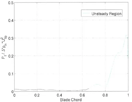
4-2 Static pressure contours at midspan of compressor B2. . . . . 4-3 Static pressure contours at midspan of compressor C. . . . . 4-4 Unsteady region is defined as area for which Pf is greater than 3% of the maximum Pf on that blade. . . . .

4-5 Instantaneous pressure profile as a sum of mechanism 1 and mechanism 2 pressure fields. . . . .. . . . . 4-6 Illustrative plot of loading unsteadiness as a sum of terms in equation 4.3. 4-7 Loading fluctuation as a sum of components in equation 4.3 for compressor

B2 main blade at 10% span and near stall operating point. . . . .

4-8 Loading fluctuation as a sum of components in equation 4.3 for compressor B2 main blade at 50% span and near stall operating point. . . . . 4-9 Loading fluctuation as a sum of components in equation 4.3 for compressor B2 main blade at 10% span and near choke operating point. . . . . 4-10 Loading fluctuation as a sum of components in equation 4.3 for compressor B2 Splitter blade at 50% span and near choke operating point. . . . .

4-11 Loading fluctuation as a sum of components in equation 4.3 for compressor BI main blade at 10% span and near stall operating point. . . . .

4-12 Loading fluctuation as a sum of components in equation 4.3 for compressor Bi main blade at 50% span and near stall operating point. . . . .

4-13 Loading fluctuation as a sum of components in equation 4.3 for compressor

4-14 Loading fluctuation as a sum of components in equation 4.3 for compressor

C main blade at 50% span. . . . 60

5-1 Illustration labeling the pressure and suction side of the diffuser vane and the sign convention for a positive inlet incidence angle. . . . . 66

5-2 Time averaged static pressure at 50% span of the compressor B2 (top) and compressor C (bottom) diffusers . . . . 67

5-3 Time averaged static pressure across one diffuser passage inlet. . . . . 68

5-4 Diffuser inlet incidence angle. . . . . 69 5-5 Close view of diffuser leading pressure contours showing small region of

reversed vane loading. . . . . 70

5-6 Correlation between pressure variation across diffuser inlet, time averaged, static pressure and amplitude of pressure fluctuation at 98% chord of im-peller blade. Comparison is made at 50% span. . . . . 71

5-7 Pressure due to mechanism 1 (left) and 2 (right) versus time for each side of the impeller blade. Measured at 93% chord and 50% span. . . . . 73

5-8 Demonstration of the measurements of values listed in table 5.2. . . . . . 76

5-9 Illustration of the variation in phase angle between mechanism 1 and

2 along the blade chord. . . . . 77

5-10 Comparison of L5 and the mechanism 2 pressure wave on the pressure

surface at one time instant for compressor C. . . . . 78

5-11 Comparison of L4t and the mechanism 2 pressure wave on the pressure

surface at one time instant for compressor C. . . . . 79

A-1 Mass flow at inlet and outlet versus main blade passings. . . . . 87

A-2 Loading unsteadiness measured from preliminary TURBO solutions

List of Tables

2.1 Summary of key design differences for each compressor. . . . . 29

3.1 Computational and experimental measurements compared with Euler tur-bine equation. . . . . 40

5.1 Pressure variation across diffuser inlet, time averaged, static pressure and amplitude of pressure fluctuation at 98% chord of impeller blade. Comn par-ison is made at 50% span. . . . . 72

5.2 Comparison of terms from equation 5.13 between the 93% and 98%

Nomenclature

Abbreviations

CFD Computational Fluid Dynamics

ETE Euler Turbine Equation

HCF High Cycle Fatigue

PIV Particle Image Velocimetry

PS Pressure Side

SS Suction Side

Symbols

A Area

c, Specific heat capacity at constant pressure

L Impeller blade loading per unit area

L Time averaged component of loading fluctuation

Lf Amplitude of loading fluctuation over time

Measure of the effect of phase angle on Lf

uor

Nd Nunber of vanes in stationary (diffuser) row

Ni Number of blades in rotating (impeller) row

P Static pressure

P Time averaged component of static pressure

P2 Mechanism 2 static pressure component

Pf Amplitude of static pressure fluctuation over time 'PPS Static pressure on pressure surface of impeller blade

P38 Static pressure on suction surface of impeller blade

qj Solution variable on i surface

r Impeller radius

t Time

T Time period of fluctuation Tt IStage inlet total temperature nO Tangential velocity component

Greek

a Flow angle

av Diffuser vane angle

j Momentum averaged incidence angle

A Acoustic wavelength

7 Stage total to total pressure rise

T Stage total to total temperature rise

#

p Density

w Diffuser vane passing radian frequency

Chapter 1

Introduction

1.1

The Centrifugal Compressor

The centrifugal compressor is a mechanical device that increases the static pressure and stagnation enthalpy of a fluid stream. Figure 1-1 depicts the two main coumpo-nents of a centrifugal compressor: the rotating impeller and the stationary diffuser. Within the impeller passage the total pressure of the fluid is increased by two dom-inant means. A centrifugal force in the stream-wise (radial) direction increases the static pressure, and the flow is accelerated in the tangential direction. Downstream of the impeller is the diffuser which recovers additional static pressure from the high

tangential velocity through a diffusion process.

The primary alternative to the centrifugal compressor is the axial compressor.

Unlike the centrifugal compressor, the axial uses a diffusion process to achieve a

static pressure rise in both its rotating and stationary components. This diffusion

process is depicted in figure 1-2. In a reference frame locked to the blade row fluid is turned to a more axial direction. This is perceived by the fluid as an area increase

and the static pressure rises through diffusion. The degree of diffusion that can be achieved in a single stage is limited by the flow separation on the suction side of the airfoil. Centrifugal stages can achieve higher pressure ratios per stage because the centrifugal impeller does not rely on diffusion alone, but also on a centrifugal

rotation >>>

hub

vlee s

.vanddlittuser

Figure 1-1: Schematic of typical centrifugal impeller and vaned diffuser from Krain [11].

pressure ratios as high as 10 to 1 [10, pg. 426] for a single stage, while a typical axial compressor would require around 9 stages to achieve the same pressure rise [6, pg. 48]. Drawbacks to the use of centrifugal compressors include an efficiency reduction of about 4-5% [10, pg. 425] and a larger frontal area which is undesirable in high performance aircraft applications in which it increases drag.

Centrifugal compressor designs are selected when cost is a key perforrnance metric. With the ability to achieve high pressure ratios in single stages, centrifugal compres-sors can be designed with fewer stages than axial comprescompres-sors for the same overall pressure ratio. Fewer stages in a design reduces complexity, part count, and cost. An inhibitor to low cost is high cycle fatigue (HCF) of compressor blades which con-stitutes a major concern to design engineers. The focus of the research described in

this thesis is on the high frequency forcing function due to impeller-diffuser unsteady

Rotor Stator V1 W2' V2 NW2 V1. Bade row velocity V3 IW3 WV<W2' W2<W3

Figure 1-2: Depiction of a stream tube through a rotor (left) and stator (right) of an axial

compressor. In reference frames locked to the blade row the turning of the flow towards the axial direction increases the stream tube area and the flow is diffused.

1.2

High Cycle Fatigue

High cycle fatigue is the reduction of mechanical strength due to a high number (greater than 103) of stress cycles [3, pg. 265]. Centrifugal impeller blades

experi-ence fluctuating stresses at high frequencies during vibration. There are two types of

blade vibration: flutter and forced. Flutter vibrations occur when there is a dynamic

instability in the interaction between the flow field and blade displacement. Forced vibration is due to an unsteady flow field created by interaction between adjacent

blade rows with relative motion. For example, wakes from an inlet guide vane are

perceived as an unsteady inlet flow to a rotating impeller directly downstream.

An-other type of interaction occurs when adjacent rows are in close enough proximity to

interact with each others potential field. This research will focus on force vibration due to interaction with the potential field from a downstream blade row. This forcing occurs at a frequency equal to the engine rotational frequency times an integer mul-tiple of the blade count. This product can be on the order of 105 per minute which

classifies this as HCF.

The amplitude of blade vibration can be greatly enhanced under resonant condi-tions. Any blade geometry has a set of modes each with a discrete natural frequency and displacement pattern. When a forcing frequency matches a particular natural frequency the corresponding mode can be excited and resonance can occur. The am-plitude of resonant response will be set by the blade material damping and correlation between the mode shape and the forcing function shape. A standard design practice to avoid resonant response is to use a Campbell diagram shown in figure 1-3. The blue lines are the natural frequencies of the blade and the red lines are integer multiples (usually blade count) of the engine operating frequency. At operating speeds which these lines cross, resonance can occur. While it is useful to know where resonance may occur, it is often hard to avoid all crossings over the operating range of a compressor. It is not known which resonant crossings are most important to avoid because the Campbell diagram incorporates no information about the correlation between mode shape and forcing shape. This research focuses on characterizing the forcing func-tion distribufunc-tion and magnitude to develop an understanding of when aeromechanic difficulty may occur.

1.3

Computational Tools

Early studies conducted on the flow field within turbomachinery were mainly ana-lytical or experimental and focused on specific regions of the compressor that could be measured. Recently more studies have employed computational fluid dynamics or CFD to solve complex models of compressor flow. Increased use of CFD is due to advances made in algorithms for solving partial differential equations and availability of computer resources; these allow large scale computations of adequate accuracy to be performed in reasonable tine frames. These simulations compute detailed flow quantities throughout the entire compressor domain and allow an in-depth interro-gation of flow processes of interest. While CFD is a powerful tool it is still based on many assumptions and therefore must be assessed against experimental data.

Ground Design Idle Speed Mode 3 25E 102E U. Mode 1 1OE

Percent physical speed

Figure 1-3: Typical Campbell diagram used to predict operating speeds where resonance

may occur [13].

1.4

Previous Work

Many studies have been conducted in an effort to understand the flow field within the centrifugal compressor. The following studies are those that have provided a conceptual and experimental base for this research to build on.

Shum studied the effect of impeller-diffuser gap size on stage performance [12]. He showed that as gap size is reduced slip is reduced, flow blockage is reduced, and tip leakage mass flux is increased. Performance increases with a reduction in slip and flow blockage but decreases with an increase in tip leakage flow. This led to the conclusion that the trend of compressor performance with impeller-diffuser gap size is not monotonic and there is an optimum gap size that maximizes stage performance. This gap size was shown to be close to 9.2% of the impeller radius which is small enough that significant unsteady interaction will occur between the impeller blade trailing edge and the pressure field of the diffuser vane leading edge. The stages examined in the present study have impeller-diffuser gap sizes close to or smaller

than 9.2% of the impeller radius.

Gould performed numerical experiments using the commercial CFD code, CFX, to study the effects of impeller-diffuser interaction on unsteady blade loading [9]. He studied a stage with a small impeller-diffuser gap of about 4% of the impeller radius. He determined that there were three controlling parameters that set the unsteady loading: impeller-diffuser gap size, relative passage Mach number, and stage load-ing. Impeller-diffuser gap size sets the peak amplitude of unsteady loading, relative passage Mach number sets the spatial distribution of the pressure wave along the impeller blade, and an increase in stage loading was shown to increase the distance the unsteadiness propagated upstream in the impeller passage.

Smythe and Villanueva examined two nearly identical centrifugal compressor stages with impeller-diffuser gap sizes that differed by .55% of the impeller radius [13, 14]. Experimental measurements performed showed that for this marginal difference in impeller-diffuser gap size the amplitude of fluctuating blade stress was nearly a factor of two greater in the stage with the smaller impeller-diffuser gap. It was observed by Villanueva that there was a correlation between the increase in unsteadiness at the diffuser leading edge and the unsteadiness at the impeller trailing edge when the impeller radius was increased.

Gallier and Cukurel acquired unsteady flow measurements of a centrifugal com-pressor stage [4, 7]. These measurements include the steady static pressure field on the shroud side of the impeller-diffuser gap, unsteady static pressure field on the hub side of the impeller-diffuser gap, Particle Image Velocimetry (PIV) flow velocity measurements in the impeller-diffuser gap and diffuser vane passage, and stage per-formiance. These detailed flow measurements in the vaneless space are used to assess computational tools by comparing metrics that are closely related to unsteady blade loading.

1.5

Technical Objectives

The objective of this study is to improve understanding of how compressor design

and operating parameters set the aerodynamic forcing function responsible for

un-steady blade loading. The approach taken is to first assess the adequacy of numerical simulations by comparing them to experimental data. Next, the numerical data is interrogated to explain the unsteady loading phenomenon. The experimental data acquired by Gallier and Cukurel and computational data from Smythe have been made available for this research. Smythe's computational data was generated using the research code TURBO. This computational data was not assessed against exper-imental data because there was insufficient experexper-imental data available on Smythe's compressor. This study will use experimental data from Gallier and Cukurel to assess both Snmythe's primary computational tool, TURBO, and the primary computational tool of this study, Fine Turbo. Given the resources available and the knowledge base built thus far, three specific technical objectives are put forth.

1. Assess the adequacy of two computational tools, TURBO and Fine Turbo to compute the flow features important to unsteady blade loading due to

impeller-diffuser interaction.

2. Identify the fluid mechanic mechanisms which set the distribution and umagni-tude of unsteady loading and their relative significance.

3. Explain the trends of the most significant mechanisms identified with operating

point and stage geometry.

1.6

Thesis Contributions

The specific contributions of this thesis fall under two categories. The first are those

pertinent to computational modeling of unsteady loading.

* CFD data is generated using the commercial code, Fine Turbo, aid compared

capa-ble of capturing the trends of the measured flow field, but errors of up to 14% exist between absolute values of flow quantities. Evidence is put forth that an inadequate turbulence model being used is the cause for the significant errors.

e CFD data generated using the commercial code, Fine Turbo, is compared against the research code, TURBO. Good agreement is demonstrated between codes.

The second category of contributions made are those that add to the conceptual understanding of unsteady loading.

" Computations on two different stages with significantly different unsteady load-ing characteristics are compared. The two most significant reasons for the ob-served differences in unsteady loading are identified. The first is die to a differ-ence in the magnitude of pressure fluctuation on the pressure side of the blade. The second is due to a difference in the wavelength of the pressure disturbance propagating upstream in the impeller passage.

" A correlation is demonstrated between the magnitude of the pressure fluctuation on the main blade surface and the strength of the non-uniformity of the diffuser inlet potential field. The strength of diffuser inlet pressure non-uniformity is set by the diffuser vane incidence angle. This indicates that the magnitude of unsteady loading can be influenced by the design and operating parameters that

set the vaneless space flow angle.

" Gould [9] identified a phase difference between the pressure fluctuation on the pressure and suction sides of the blade. In this work the effect of this phase difference is quantified and shown to be significant. It is shown that an increased wave length of pressure disturbances propagating upstream reduces the peak unsteady loading and moves the location of peak unsteadiness upstream.

1.7

Thesis Outline

Chapter 2:

This chapter describes the technical approach used to accomplish the research ob-jectives. A description of the research articles and computational tools is presented along with the motivation for choosing them. Lastly, the design of experiment is

presented.

Chapter 3:

In this chapter Fine Turbo and TURBO are assessed as computational tools. Fine Turbo results are compared to experimental measurements. TURBO results are then conipared against Fine Turbo results on a different compressor. The capabilities and limitations of each code are identified.

Chapter 4:

This chapter compares the static pressure field of multiple different compressors. The unsteady loading is quantitatively characterized. The two most significant effects responsible for the differences in unsteady loading between compressor designs are identified.

Chapter 5:

This chapter addresses the two effects identified in chapter four. The flow processes responsible for the differences are correlated with compressor design parameters.

Chapter 6:

This chapter summarizes the key findings of this thesis and discusses recommnenda-tions for future work.

Chapter 2

Technical Approach

A computational approach is used in this study because of the difficulty in measuring detailed metrics that would characterize unsteady blade loading. To assess the ad-equacy of a computational approach simulations are compared against the vaneless space measurements acquired by Gallier and Cukurel. Computational data is then

interrogated in detail to extract new information about unsteady blade loading.

2.1

Research Articles

This work investigates computational data from three different compressors. Each

compressor has been studied in previous investigations of unsteady blade loading. This section describes relevant characteristics of each compressor.

2.1.1

Compressor A

The first compressor, referred to as compressor A, was studied by Gould. This compressor was initially studied because unsteadiness due to the impeller-diffuser interaction was detected as far upstream as the impeller blade leading edge. The inpeller-diffuser gap of this stage is 15% of the diffuser passage width. This is the smallest impeller-diffuser gap of the compressors studied. The diffuser for this stage is a discrete passage diffuser. Ansys CFX was the computational tool used to study

this compressor. Computational results were compared against experimental data by Gould [9].

2.1.2

Compressor B

The next compressor was studied by Sinythe and Villanueva. This compressor has two design variations which will be referred to as compressors B1 and B2. These compressors are of nearly identical design with the only difference being a marginally larger impeller radius in compressor B2. This compressor was studied to explain the high sensitivity of blade response to impeller diffuser gap size measured on a test rig. The gap to diffuser pitch ratio is about twice that of compressor A. The diffuser for these stages is a cambered vane. The research code TURBO was used to analyze these stages. In Smythe's and Villanueva's studies there was only a limited amount of test rig data available to compare with CFD results and thus it is still necessary to assess the adequacy of these computations before using them to draw conclusions on the trends of unsteady loading [13,14].

2.1.3

Compressor C

The last stage to be interrogated is compressor C. This compressor is selected for study because unsteady experimental measurements were acquired in the vaneless space by Gallier and Cukurel. The source of the unsteady flow field is the interaction between the impeller and diffuser that occurs in the vaneless space. Availability of flow measurements in this region enables a direct assesimient of the capability of computations to capture the unsteady flow field. In this work numerical computations are conducted on this stage using Numneca Fine Turbo. Compressor C has a vane wedge diffuser and a gap size similar to compressors B1 and B2 [5, 7]. Table 2.1 summarizes key design features of each compressor.

A B1&B2 C

Gap to Pitch Ratio .15 .30 .30

Diffuser Type Discrete Passage Cambered Vane Wedged Vane

Impeller Backsweep Not Available Low High

Table 2.1: Summary of key design differences for each compressor.

2.2

Numeca Fine Turbo

Numeca Fine Turbo is the primary computational tool used in this study. Fine Turbo solves the unsteady Reynolds-Averaged Navier-Stokes equations over a discretized approximation of the compressor doimain. Fine Turbo uses a finite volume scheme that is 2nd order accurate in both space and time [1]. Turbulent flow is modeled with a k-c turbulence model. This model is chosen to keep consistent with the model used by Smythe in her TURBO computations.

2.2.1

Phase-Lagged Boundary Condition

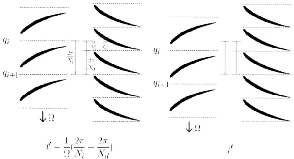
A particular advantage to using Fine Turbo is its ability to apply a phase-lagged boundary condition for circumferentially periodic geometries. The phase-lagged bound-ary condition assumes that all flow variables on the circumferential boundbound-ary of a blade passage are periodic with the passing of the adjacent blade row. This assump-tion allows for a significant reducassump-tion in computaassump-tional effort to be achieved by only modeling one blade passage for each row. The phase-lagged boundary condition is

depicted in figure 2-1 for two blade rows with spacing that differs by g - -. Ni

and Nd are the blade counts for the rotating and stationary blade rows respectively. Notice that the surface qj at time t' is in the same position relative to the stationary

blade row as surface qj+1 at time t' - '(' - '). The relation for any flow variable

on these surfaces can be written as:

qi(t')=q+1 t'- 1((2.1)

I

---

---/00

---/00

Figure 2-1: Depiction of phase-lag boundary condition. Surface qi at time t' is set equal

to surface qi+1 at time t' - - )2

Chen [15] gives a general form of this relationship for both the rotating and sta-tionary rows.

q (t') = qjot ' +

qt'at'r(t') = _qi+M qtator _i t'

m27 \QiNi m 2 -r |0|_Ni n2-F + _{n27r )}INd) |IN Q) \ (2.2) (2.3)

where m and n are integers of either sign. An implication of the phase-lag as-sumption is that flow features occurring at frequencies less than the blade passing frequency are not captured. Experimental data from Gallier shows that dominant frequencies are at or above the main blade passing frequency [7]. This indicates that the phase-lagged approximation is appropriate.

2.2.2

Computational Tool Selection

In this study computations are implemented on compressors C and B2, aid the results are compared to computational data generated by previous researchers. While it

---

---Nk**

---

--

---

-would be advantageous to use one of the _{same CFD tools used in previous studies,}

Fine Turbo is selected for use as a new code for several reasons. Fine Turbo is selected over CFX because CFX cannot implement the phase-lagged boundary condition' . Using CFX would either require imodifying the compressor blade counts so that a periodic boundary condition could be used or resorting to a full annulus calculations. Fine Turbo was selected over TURBO due to fast convergence using a multigrid scheme and its far more robust operation. Appendix A gives additional details on why TURBO is not the primary computational tool of this study. Because results from different codes are compared, the method for assessing simulations must include a comparison between CFD codes.

2.3

Computational Domain

The computational grid of compressor B2 is the same grid used by Smythe. It is a structured H pattern grid with about 0.8 million nodes and 5 blocks. The com-putational grid used for coumpressor C is a structured H-0-H patterned grid with approximately 3.5 million nodes and 29 blocks. The grid structure of compressors B2 and C are shown in figures 2-2 and 2-3 respectively. The H-a-H pattern grid is comprised of 0 sections which are blocks with grids that are aligned with the blade surface and H sections which fill the rest of computational domain with a grid aligned with the flow path direction. The H-a-H grid structure allows better orthogonality at the blade surfaces where this is important to accurately capture boundary layers. A draw back to this grid structure is its complexity. H-a-H grids often contain a large number of blocks with non-uniform block orientation. This complicates the pre and post processing of computational data.

'At the time of the CFD code selection the current CFX version was 13.0. In December 2011 CFX version 14.0 was released with a provision to apply phase-lagged boundary conditions [2].

Figure 2-2: Structured H grid of compressor B2.

\

\\

\

\

2.4

Computational Procedure

To initialize the unsteady computations, mixing-plane computations are performed

first. The mixing plane approximation circumferentially mixes the flow exiting the

impeller and then applies it as a circunferentially uniform inlet boundary condition to the diffuser [1]. This method reduces the computation to a steady one, and therefore requires less computational resources. Information about unsteady processes may not be gained from this type of simulation, however it is capable of approximating stage

performance. The procedure for generating full unsteady solutions is to implement

mixing-plane computations along a full speed line to compare with test rig data. Then a specific operating point of interest is chosen for implementing full unsteady calculations. The mixing plane solution at this operating point is used as an initial

condition to the unsteady calculation.

2.5

Compressor C Experimental Data

The primary reasons for selecting compressor C as a, research article is that there is a wealth of experimllental data available in the vaneless space of the compressor. Data was collected by Gallier at three different operating points on two different speed lines (6 operating points total) plotted in figure 2-4. The 2 speed lines chosen are at

100% and 90% of design speed. The 90% speed line is chosen because a structural

analysis shows a resonant crossing on the Campbell diagram at this speed [8]. Stage performance measurements include inlet and outlet total temperature, total pressure, and static pressure. Vaneless space measurements include steady pressure on the hub side and unsteady pressure measurements from the shroud side of the vaneless space. The steady and unsteady static pressure are measured via arrays of pressure transducers shown in figure 2-5. Particle Image Velocinetry (PIV) measurements were also acquired on the 90% speed line at the operating point indicated in figure

2-4. PIV measures the velocity field through an optical window on the shroud side of the compressor. Figure 2-5 shows the region that the velocity is measured. This data

-r- T

Experimental 90% speed line

- x Experimental 100% speed

* Fine Turbo Mixing Plane 90% speed

- O Fine-Turbo Unsteady 90% speed

0.95- 0.9-0.85F _availablePlVdata 0.8F 0.75 0.8 0.85 Figure 2-4: Compressor

data are available.

0.9 0.95

Mass Flow

C operating points where experimental data and conputational

is available at 6 different spans and 10 different time delays during one blade passing.

2.6

Simulation Assessment

It is a technical objective of this research to assess both the TURBO computations performed by Smythe and the Fine Turbo computations performed on compressor C. An indirect method for assessing TURBO data is adopted because of the difficulty in implementing TURBO computations on compressor C. Fine Turbo computations are assessed against experimental data on compressor C. Once this comparison showed that Fine Turbo was capable of capturing features related to unsteady loading, Fine Turbo computations are run on compressor B2. TURBO results generated by Smythe are then assessed against Fine Turbo computations.

The comparison between Fine Turbo computations and experimental data is made at the operating point where PIV data is available. A series of mixing plane simula-tions are run to match the 90% speed line using the experimentally measured inlet

1.1 1.05 1 Ir 0 0 I-1.05 1.1 5 -- r- I I 0 0 1

Hub

_Shroud

Figure 2-5: Steady pressure probe locations on hub side (left). Unsteady pressure probe

and PIV optical window location (right)

total pressure and temperature as boundary conditions to the computation. Each op-erating point along the speed line is achieved by adjusting the back pressure. Figure 2-4 shows that the computed pressure rise is about 10% greater than the measured value. An unsteady simulation is then run at an operating point midway between choke and stall to compare the unsteady flow in the vaneless space. This operating point is shown in figure 2-4. To compare computational and experimental operating points that have the same relative speed line locations (midway between choke and stall) a higher back pressure must be used in the simulation due to the 10% difference in the computed and measured pressure rise.

To assess TURBO computations on compressor B1 and B2 Fine Turbo is run at the near stall operating point labeled in figure 2-7 on compressor B2. This compressor and operating point is chosen because the unsteady loading is most significant.

2.7

Design of Experiment

The primary objective of this work will be to better understand the trends of unsteady loading with design parameters. When comparing two test cases it is desirable to only have one design parameter varied. With the need to assess computational tools with experimental data in this study, compressors were selected based on the availability of data and not their similarities or dissimilarities in design parameters. In addition to multiple design parameters being varied across compressors, data is only available at

Stage Pressure Ratio

Available

"OData

Corrected Mass Flow per-unit-area (inlet)

Figure 2-6: Operating point at which unsteady data is available on Compressor A [9].

operating points that differ across compressors. An argument must be made that the differences in unsteady loading characteristics across compressors are due to design parameters and not operating point. This is done by comparing unsteady solutions at multiple operating points on the same compressor. The features common across different operating points but different across stages are deemed the effects of design parameters. Reasoning is then put forth as to which design parameters are responsible for the results observed and why. Figure 2-6 shows the near stall operating point where unsteady data is shown for compressor A. Figure 2-7 plots the operating points where unsteady data is available on compressor B1 and B2.

2.8

Summary

The technical approach used to accomplish the research objectives stated in chapter 1 is described. To assess the ability of both Fine Turbo and TURBO to capture the flow features relevant to unsteady loading Fine Turbo computations are run on compressor C and compared against experimental measurements. Fine Turbo computations are

TURBO and Fine Turbo 1.02 0 0.98 M 0.96 0 0.94 0.92 B2 Bi 1.02 Normalized 1.04 S

Figure 2-7: Operating points at

Turbo in compressors B1 and B2.

which unsteady data is available in TURBO and Fine

then conducted on compressor B2 and compare against TURBO computational data.

Once the capabilities and limitations of CFD are deternined the computational data

from compressor A, Bi, B2, and C are assessed to enable a general characterizations of unsteady loading.

TURBO only

0.9

Chapter 3

CFD Assessment

Two steps are taken to assess the capability of Fine Turbo and TURBO to capture the flow features relevant to unsteady loading. First, Fine Turbo unsteady results on compressor C are compared to the experimental data. Next, Fine Turbo and TURBO unsteady results are compared on compressor B2.

3.1

Fine Turbo Vs Experimental: Time Averaged

Stage performance metrics are compared to give a broad view of CFD's capabilities and limitations in computing the flow field. This comparison is conducted at the data point on the 90% speed line where PIV data is available. Table 3.1 lists the time averaged total to total temperature ratio (r), total to total pressure ratio (-r), and corrected mass flow (rneo,). In each case the computed values are higher than the experimental. It is known that CFD is capable of computing stage temperature ratio accurately, therefore this error is interrogated further by comparing to the Euler Tur-bine equation (ETE). The ETE uses conservation of energy and angular momentum to relate the shaft work done by the compressor to the total temperature rise across the impeller [10].

r = 1-+ (3.1)

Fine Turbo Unsteady Experimental % error r 3.518 3.260 7.9% uo 2.128 kg/s 1.864 kg/s 14.2% Tr 1.569 1.489 5.4% U02 316.2 n/s 329.4 m/s 4.0% T from ETE 1.558 1.582 .4%

% error from ETE 0.7% 5.9%

Table 3.1: Computational and experimental measurements compared with Euler turbine

equation.

Q is the rotational speed of the impeller in radians per second, 02 is the mass

aver-aged tangential velocity at the impeller exit, r is the radius at which U02 is measured, c, is the specific heat at constant pressure, and Ttj is the total temperature at the compressor inlet. To evaluate the ETE, knowledge of the vaneless space flow velocity is needed. Figures 3-1 and 3-2 are the Mach number and flow angle in the vaneless space from CFD and PIV data. U92 can be computed directly from CFD data. For

the experimental case, U02 is estimated by taking the spanwise average of the flow

quantities and using the mean acoustic speed of 411 m/s [8]. Table 3.1 shows values of U02 and T computed from the ETE for the CFD and experiment cases. The percent error between the CFD computed temperature ratio and the ETE equation is 0.7%,

while the percent error between the experimentally measured temperature ratio and the ETE is 5.9%. This suggests error in either the outlet total temperature

mea-surement or the PIV meamea-surements. Decemit agreement between the PIV measured

quantities with computations in figures 3-1 and 3-2 gives evidence to the error being in the total temperature measurement.

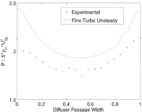
Figure 3-3 compares time averaged static pressure at a distance 8% of the diffuser pitch (circumferential distance between diffuser vane leading edges) upstream of the diffuser inlet. The comparison shows that CFD captures the pressure distribution,

but the computed performance is about 10% higher. The higher static pressure shown in figure 3-3 and the agreement in Mach number shown in figure 3-1 indicates a higher computed total pressure in the vaneless space and thus higher impeller efficiency.

0.2 0.4 0.6

Span (Hub to Shroud)

0.8 1

Figure 3-1: Vaneless space Mach number versus span [8].

25 111

0.2 0.4 0.6

Span (Hub to Shroud) 0.8 1 Figure 3-2: Vaneless space flow angle versus span [8].

1 0.8 0.60.4 - a-E z C.O M Experimental

Fine Turbo Unsteady

0.2 0' 0 20 15 10- 5- 0- -5- 10-CD M -2₀ 0 0) 0 Experimental

Fine Turbo Unsteady

-15 0

2.5

Cl

2-1.51I

0 0.2 0.4 0.6 0.8 1

Diffuser Passage Width

Figure 3-3: Vaneless static pressure comparison.

3.2

Fine Turbo Vs Experimental: Unsteady

To determine the reason for the higher computed impeller efficiency, vaneless space Mach number is compared at discrete time instants. Figure 3-4 shows the measured and computed Mach contours at two different times. The jet-wake flow structure described by Dean [6] is seen from the PIV measurements. As flow enters the inducer, relative frame velocity is higher on the suction than the pressure side. The suction side high velocity fluid separates before exiting the impeller. Downstream of this separation the gradient of momentum across the impeller passage switches, with fluid momentum now being higher on the pressure side. When translating relative frame velocity to the absolute frame, the gradient of momentum across the impeller passage is reversed because the direction of blade backsweep is opposite to the direction of rotation. This results in the high momentum region leaving the suction side of the impeller in the absolute frame. While figure 3-4 indicates that the computations capture the jet-wake structure and the approximate Mach number magnitude, the distribution of Mach number is significantly different. Figure 3-5 plots the absolute

Experimental

Figure 3-4:

simulation

Comparison of absolute frame Mach contours between Purdue PIV data and

frame Mach number across the exit of one blade passage at one time instant. The mean Mach number is captured, however the gradient of Mach number from the suction to pressure side is significantly steeper in the experimental case. This gradient is set by the degree of separation that occurs on the suction side of the impeller blade. Flow in low momentum or separated regions can be highly sensitive to the turbulence model used. It is suggested that the k-E turbulence model is under computing the degree of separation that occurs on the suction side of the impeller.

Additional evidence indicating the inadequacy of the k-e turbulence model can be gained from figure 3-2. There is good agreement in flow angle near the hub surface, however toward the shroud the flow angle is lower in the experimental case. Lower flow angle on the shroud side is due to the separation of flow over the concave shroud surface. Computations under predict the degree of separation that occurs and thus compute a higher flow angle near the shroud.

From these observations it is suggested that there is significant error in the CFD solutions due to an inability to capture the turbulence sensitive flow processes that occur on the suction side of the impeller blade and shroud surface. Loss and the

PIV Data FineTurbo Unstead

t=1/10 T t=1/11 T

t=6/10 T t=5/11 T

1.1--- -

----41

0.9

0 .8 * _Experimental

Fine Turbo Unsteady

0.7-0.6

0.5 '

0 0.2 0.4 0.6 0.8 1

Impeller Passage Width (PS to SS)

Figure 3-5: Absolute frame Mach number at impeller exit and t-5/11T.

degree of separation is under predicted by CFD leading to the over prediction of vaneless space static pressure, stage pressure ratio, and corrected mass flow. Despite these significant offsets, the flow structure in the impeller passage and vaneless space is captured, thus the computational results are useful for determining the trends of unsteady loading with design and operating parameters.

3.3

TURBO Vs Fine Turbo Comparison

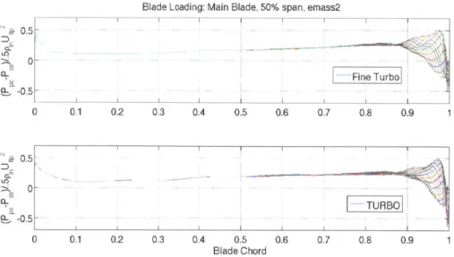
Fine Turbo computations are implemented at the near stall operating point of the B2 compressor. This operating point is chosen because the amplitude of unsteady loading is highest. Unlike the comparison with experimental data, flow quantities are available throughout the entire computational domain. Therefore a more direct comparison of the computation of unsteady loading can be made. The instantaneous loading is the difference between the pressure on the pressure and suction side of the blade. Figure 3-6 plots the instantaneous loading at each time step for Fine Turbo and TURBO and shows that there is good agreement between the two codes. Figure

Blade Loading: Main Blade, 50% span, emass2 0 -Fine Turbo -0.5-0 0.1 0.2 0.3 0.4 0.5 0.6 0.7 0.8 0.9 1 -0.5 0-Q -0,5--0 0.1 0.2 0.3 0.4 0.5 0.6 0.7 0.8 0.9 1 Blade Chord

Figure 3-6: Comparison of unsteady loading computed by Fine Turbo and TURBO.

3-7 plots the amplitude of the pressure fluctuation for each code on the pressure

and suction side of the blade. Again, good agreement exists between the two codes.

Fine Turbo computes a pressure side peak unsteadiness that is 3% of the dynamic head higher, however the distribution of unsteadiness is nearly identical. This result indicates that TURBO is subject to the same capabilities and limitations determined for Fine Turbo.

3.4

Summary

Fine Turbo and TURBO are assessed as computational tools for computing the flow features relevant to unsteady impeller blade loading. CFD is shown to over predict time averaged temperature ratio, pressure ratio, mass flow, and vaneless space static pressure by as high as 14%. The error between computed and measured temperature ratio is shown to be due to experimental error in the temperature measurement. An interrogation of instantaneous flow quantities gives evidence that the k-e turbulence model currently used is responsible for the over prediction of stage pressure ratio, mass flow, and vaneless space static pressure. Despite the over prediction in absolute flow quantities the distribution of the flow is captured by CFD. It is thus concluded

Pressure Unsteadiness --- Fine Turbo PS TURBO PS Fine Turbo SS TURBO SS b ~ /7 I, 0.4 0.5 0.6 0.7 0.8 0.9 1

Main Blade Chord

Figure 3-7: Comparison between Fine Turbo and TURBO computations of

tuation on the pressure and suction side.

pressure

fluc-that CFD is an adequate tool for computing relative differences in unsteady loading between different design and operating conditions. A comparison is made between TURBO and Fine Turbo that shows the near identical agreement. This indicates that TURBO is subject to the same capabilities and limitations determined for Fine Turbo. 0.8 0.7 F cl L E Qa 0.6 0.5 0.4 0.3 0.2 0.1 iL 0 I

Chapter 4

Characterization of Unsteady

Loading

In chapter 3 it is shown that TURBO and Fine Turbo are adequate tools for com-puting relative differences in unsteady loading between different design and operating conditions. In this chapter the computed static pressure field of each stage is inter-rogated to characterize the unsteady blade loading. First the static pressure field is examined at discrete time instants to identify a set of unsteady loading mechanisms that are common to all stages. A quantitative analysis is then presented to measure the relative significance of each mechanism. Finally, the results of this analysis are compared across two of the compressors. The differences in unsteady loading between the two stages are explained in terms of the most significant mnechanisms.

4.1

Unsteady Static Pressure Field

Figures 4-1, 4-2, and 4-3 are midspan static pressure contours at six different time instants for compressor A, B2, and C. T is the time period of one main blade pass-ing. The static pressure field shown for compressor B2 is at the near stall operating

point, however it is qualitatively representative to all other operating points on both

B compressors. Static pressure fields for compressor B2 and C show there is a steady region far upstream in the impeller passage. The pressure field in this region is

dom-inated by the Coriolis force. The pressure varies with a near constant gradient in the circumferential direction with higher pressure on the pressure surface of the blade. Downstream of this is an unsteady region where the pressure distribution transitions from being dominated by the Coriolis force to the potential field of the downstream dif-fuser vanes. This is the region in which the flow mechanisms responsible for unsteady loading occur. This chapter will quantify the extent of this region and magnitude of unsteadiness on the blade surface. The static pressure distribution for compressor A differs from that of compressors B2 and C. There is no distinguishable steady region upstream (Gould shows there is significant unsteadiness all the way upstream to the blade leading edge [9]). In all compressors significant unsteadiness in pressure on the impeller blade tip is a result of the impeller blade passing through the diffuser vane potential field.

In examining figures 4-1, 4-2, and 4-3 two distinct mechanisms that contribute to unsteady loading can be identified.

1. Mechanism 1: As the blade sweeps through the non-uniform potential field of the diffuser, it experiences a high pressure when in close proximity to the diffuser leading edge stagnation region and a lower pressure when in between diffuser

vanes.

2. Mechanism 2: As the blade passes the diffuser vane, pressure waves develop at the impeller blade trailing edge and propagate upstream.

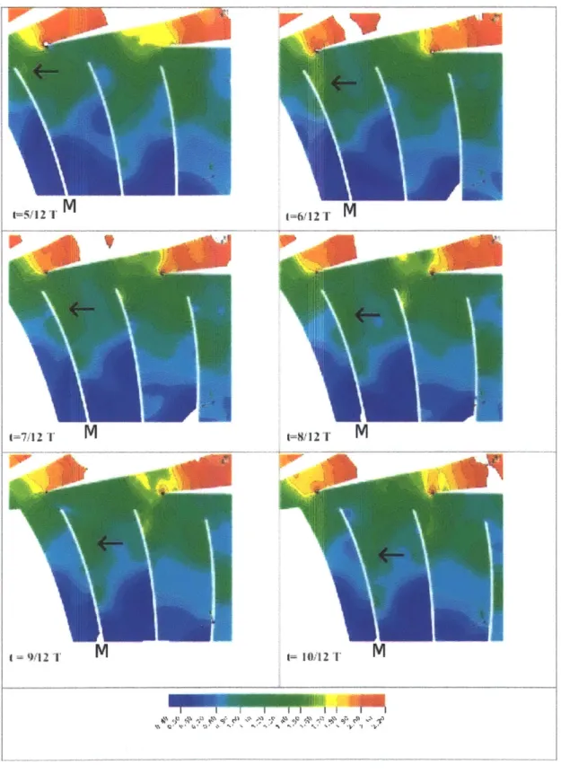
Mechanism 1 is observable in all three compressors. This mechanism is elucidated in figure 4-2. When t = 5/12T the main impeller blade (marked by an M) is aligned with a diffuser vane and the static pressure around the impeller blade tip is relatively high. When t = 9/12T the impeller main blade is between diffuser vanes and the static pressure around the blade tip is relatively low. This observation suggests that the level of non-uiformity of the diffuser inlet potential field is proportional to the pressure unsteadiness on the blade surface.

Mechanism 2 is elucidated in figure 4-1. As the main blade passes by the diffuser

t-8/12T M

L. _-9

9

- W12 T 2 T

Figure 4-1: Static pressure contours at midspan of compressor A. 1=7/12 T

M M t=5/12 T M t=7/12 T M t=6/12 T M t=8/12 T M t=9/12 t=10/12 1.3 ,02.3 1.4 1.6 1.8 2 2.2 P / .5*rho*UtipA2

Figure 4-2: Static pressure contours at midspan of compressor B2.

M t=4/11 T M t=6/11 T M t=8/11 T 1.3 2.3 1.4 1.6 1.8 2 2.2 P / .5*rho*UtipA2 t=3/11 T M t=5/11 T M t=7/11 T

Figure 4-3: Static pressure contours at midspan of compressor C. m