Publisher’s version / Version de l'éditeur:
International Society for Photogrammetry and Remote Sensing, 2004
READ THESE TERMS AND CONDITIONS CAREFULLY BEFORE USING THIS WEBSITE. https://nrc-publications.canada.ca/eng/copyright
Vous avez des questions? Nous pouvons vous aider. Pour communiquer directement avec un auteur, consultez la première page de la revue dans laquelle son article a été publié afin de trouver ses coordonnées. Si vous n’arrivez pas à les repérer, communiquez avec nous à [email protected].
Questions? Contact the NRC Publications Archive team at
[email protected]. If you wish to email the authors directly, please see the first page of the publication for their contact information.
NRC Publications Archive
Archives des publications du CNRC
This publication could be one of several versions: author’s original, accepted manuscript or the publisher’s version. / La version de cette publication peut être l’une des suivantes : la version prépublication de l’auteur, la version acceptée du manuscrit ou la version de l’éditeur.
Access and use of this website and the material on it are subject to the Terms and Conditions set forth at
Automatic Correspondences For Photogrammetric Model Building
Roth, Gerhard
https://publications-cnrc.canada.ca/fra/droits
L’accès à ce site Web et l’utilisation de son contenu sont assujettis aux conditions présentées dans le site LISEZ CES CONDITIONS ATTENTIVEMENT AVANT D’UTILISER CE SITE WEB.
NRC Publications Record / Notice d'Archives des publications de CNRC:
https://nrc-publications.canada.ca/eng/view/object/?id=cd6008a5-e818-46d8-8e2c-c428e0d6bdb8 https://publications-cnrc.canada.ca/fra/voir/objet/?id=cd6008a5-e818-46d8-8e2c-c428e0d6bdb8National Research Council Canada Institute for Information Technology Conseil national de recherches Canada Institut de technologie de l'information
Automatic Correspondences For Photogrammetric
Model Building *
Roth, G.
October 2004
* published in the XXth Congress. International Society for hotogrammetry and Remote Sensing. Istanbul, Turkey. July 12-23, 2004. Commission V, pp. 713-720. NRC 47392.
Copyright 2004 by
National Research Council of Canada
Permission is granted to quote short excerpts and to reproduce figures and tables from this report, provided that the source of such material is fully acknowledged.
AUTOMATIC CORRESPONDENCES FOR PHOTOGRAMMETRIC MODEL BUILDING
Dr. Gerhard Roth
Computational Video Group, Institute for Information Technology National Research Council of Canada
[email protected] Working Group TS ICWG V/III
KEY WORDS: Photogrammetry, Modelling, Matching, Automation, Feature, Semi-Automation. ABSTRACT
The problem of building geometric models has been a central application in photogrammetry. Our goal is to partially automate this process by finding the features necessary for computing the exterior orientation. This is done by robustly computing the fundamental matrix, and trilinear tensor for all images pairs and some image triples. The correspondences computed from this process are chained together and sent to a commercial bundle adjustment program to find the exterior camera parameters. To find these correspondences it is not necessary to have camera calibration, nor to compute a full projective reconstruction. Thus our approach can be used with any photogrammetric model building package. We also use the computed projective quantities to autocalibrate the focal length of the camera. Once the exterior orientation is found, the user still needs to manually create the model, but this is now a simpler process.
1 INTRODUCTION
The problem of building geometric models has been a cen-tral application in photogrammetry. Our goal is to make this process simpler, and more efficient. The idea is to au-tomatically find the features necessary for computing the exterior orientation for a given set of images. The claim is that this simplifies the model building process. To achieve this goal it is necessary to automatically create a reliable set of correspondences between a set of images without user intervention.
It has been shown that under certain conditions it is pos-sible to reliably find correspondences, and to compute the relative orientation between image pairs. But these con-ditions are that the images are ordered, and have a small baseline, such as those obtained from a video sequence. However, in photogrammetric modeling the input images are not ordered and the baseline is often large. In this case it is necessary to identify which image pairs overlap, and then to compute correspondences between them.
Our solution to this problem contains a number of inno-vations. First, we use a feature finder that is effective in matching images with a wide baseline. Second, we use projective methods to verify that these hypothesized matches are in fact reliable correspondences. Third, we use the pro-jective approach only to create a set of correspondences, and not to compute a projective reconstruction. At the end of the process these correspondences are sent to a bundle adjustment to find the exterior camera parameters. This makes the generation of the correspondences independent of the bundle adjustment. Therefore our approach can be used with any photogrammetric model building package. The computed projective quantities are the fundamental matrix between image pairs, and the trilinear tensor be-tween image triplets. The supporting matches for the ten-sors are chained across images that are found to be adjacent to create correspondence chains. We show that this process creates very reliable correspondence chains. Finally, we
use the computed projective information to autocalibrate the camera focal length.
Working in projective space has the advantage that camera calibration is not necessary. The other advantage is that it is possible to autocalibrate certain camera parameters, in particular the focal length, from the fundamental matrices. The complexity of computing the fundamental matrix, and trilinear tensor is less than that of the bundle adjustment.
2 DISCUSSION AND RELATED WORK
Model building is a very common industrial Photogram-metric application. The basic methodology has been un-changed for many years; calibrate the camera, choose the 2D projections of the 3D points of interest in different im-ages, and then run the bundle adjustment. Then take the computed 3D data points, and join them together to cre-ate the model topology. The process is very manual, but has the advantage that the user can control the exact geom-etry and topology of the final model. Recently there has been some important recent work in the area of automated model building. However, the problem of finding the ap-propriate geometry and topology is a difficult and unsolved one. Thus the photogrammetric approach to model build-ing will likely be used for a considerable length of time. However, while it is very flexible it is also very labor in-tensive.
Is it possible to partly automate the photogrammetric model building process and still leave it’s flexibility intact? We believe the answer is yes. Normally the feature points used to build the model are also the ones used to run the bundle adjustment. But what if some other automatic process had already computed the exterior orientation? Then comput-ing the required 3D data points for the model would require only triangulation, instead of the bundle adjustment. The triangulation process is inherently simpler than the bundle adjustment, so this would simplify the process of creating
the required 3D geometry. If it were possible to automat-ically find a set of features between overlapping images, then it would be possible to run the bundle adjustment, and compute the exterior orientation. In the past, such match-ing has been done only in restricted situations. These re-strictions are that the motion between the images is rela-tively small, and that there is some a-priori process which labels images as overlapping. For example, if the images were taken from a video sequence the baseline between then is small and they are also likely to have significant overlap.
If we consider the set of images that are used in a typi-cal photogrammetry project these two restrictions do not hold. The input to the photogrammetric model building process is a set of unordered images with a wide physical separation, that is with a wide baseline. There have been a number of recent attempts to compute reliable correspon-dences between such images. The most complete system (Schaffalitzky and Zisserman, 2002) is a wide baseline, un-ordered matching system that uses affine invariants as the feature descriptor. This system attempts to construct a min-imal spanning tree of the adjacency graph and it does not allow this spanning tree to form cycles. However, cycles are very important in the bundle adjustment process be-cause they reduce the propogation of errors. Another ap-proach (Ferrari et al., 2003) tries to expand on the number of correspondences between adjacent views by using the concept of tracks. The method of (Martinec and Pajdla, 2002) also has tracks, but uses a trilinear tensor to increase the number of tracks that have been found. There is also a variety of different descriptors (Baumberg, 2000, Pritch-ett and Zisserman, 1998) that have been used as features, other than the corner based approaches.
This paper describes a way of solving the wide baseline, unordered image matching problem which can interface with standardized photogrammetric packages. The input is a set of images without any intrinsic camera parame-ters, and the output is a set of correspondences between these images. These correspondences are then sent to a commercial photogrammetric package, which uses them to compute the exterior orientation of the cameras. While the bundle adjustment process requires camera calibration, the correspondence process does not. The pixel size, and aspect ratio for the camera, can be obtained from the era manufacturers data. Since many modern digital cam-eras have a zoom lens this camera parameter is not easily obtained without a formal calibration step. The automatic correspondence process also has the ability to automati-cally find the focal length of the camera. Thus our system computes the correspondences between images and auto-matically calibrates the focal length.
Our approach computes the fundamental matrix between image pairs, and the trilinear tensor between image triples. It is based on the SIFT corner detector (Lowe, 1999), which has been shown experimentally to be the most robust ner features (Mikolajczk and Schmid, 2003).. The cor-respondences that support the trilinear tensor are chained strung together in longer tracks using a breadth first search. This method allows cycles in the image adjacency graph,
and also uses a chained trilinear tensor, which makes it dif-ferent from other approaches. The idea of using chained trilinear tensors was first described in (Roth and White-head, 2000), and has been shown to create very reliable correspondences. If there are n input images one would expect the overall complexity of this process to beO(n3
). However, in practice, the complexity is actually O(m3
), wherem is the average number of images that have sign-ficant overlap with any given image. We will show ex-perimentally that m is typically about one half of n, the total number of images. ThereforeO(m3
) complexity is not excessive becausem is relatively small. A typical pho-togrammetric project has thirty images (n) and there are at most ten to fifteen overlapping images (m) for each of these thirty images. The total processing time to compute all the correspondences in such a case is about fifteen min-utes on a 2 gigahertz machine. Finally, as a by product we can use the calcuated fundamental matrices to perform autocalibration of the camera focal length.
3 ALGORITHM STEPS
The input is an unordered set of images. The output is a set of correspondences among these images. The processing is as follows:
For every image pair compute a fundamental matrix. For all fundamental matrices
that have enough supporting matches compute an associated trilinear tensor. Chain the trilinear tensor matches
using bread first search. Output the chained matches
as valid correspondences.
4 PROJECTIVE VISION
Structure from motion algorithms assume that a camera calibration is available. This assumption is removed in the projective paradigm. To explain the basic ideas behind the projective paradigm, we must define some notation. As in (Xu and Zhang, 1996), given a vector x= [x, y, . . .]T
, ˜
x defines the augmented vector created by adding one as the last element. The projection equation for a point in 3D space defined as X= [X, Y, Z]T is:
s ˜m= P ˜X
wheres is an arbitrary scalar, P is a 3 by 4 projection ma-trix, and m= [x, y]Tis the projection of this 3D point onto
the 2D camera plane. If this camera is calibrated, then the calibration matrixC, containing the information particu-lar to this camera (focal length, pixel dimensions, etc.) is known. If the raw pixel co-ordinates of this point in the camera plane are u= [u, v]T, then:
˜ u= C ˜m
whereC is the calibration matrix. Using raw pixel co-ordinates, as opposed to actual 2D co-ordinates means that we are dealing with an uncalibrated camera.
Consider the space point, X = [X, Y, Z]T
, and its image in two different camera locations; ˜x= [x, y, 1]T and ˜x′ =
[x′, y′, 1]T. Then it is well known that:
˜
xTE˜x′= 0
HereE is the essential matrix, which is defined as: E = [t] × R
wheret is the translational motion between the 3D cam-era positions, andR is the rotation matrix. The essential matrix can be computed from a set of correspondences be-tween two different camera positions using linear methods (Longuet-Higgins, 1981). This computational process has been considered to be very ill-conditioned, but in fact a simple pre-processing step improves the conditioning, and produces very reasonable results (Hartley, 1997a). The matrixE encodes the epipolar geometry between the two camera positions. If the calibration matrixC is not known, then the uncalibrated version of the essential matrix is the fundamental matrix:
˜
uTF ˜u′ = 0
Here ˜u= [u, v, 1]T and ˜u′ = [u′, u′, 1]T are the raw pixel
co-ordinates of the calibrated points ˜x and ˜x′. The
fun-damental matrixF can be computed directly from a set of correspondences by a modified version of the algorithm used to compute the essential matrix E. As is the case with the essential matrix, the fundamental matrix also en-codes the epipolar geometry of the two images. OnceE is known, the 3D location of the corresponding points can be computed. Similarly, onceF is known the 3D co-ordinates of the corresponding points can also be computed, but up to a projective transformation. However, the actual sup-porting correspondences in terms of pixel co-ordinates are identical for both the essential and fundamental matrices. Having a camera calibration simply enables us to move from a projective space into a Euclidean space, that is from F to E.
5 FUNDAMENTAL MATRICES
We are given a set ofn input images, and we want to cal-culate the fundamental matrix between every one of these n2
image pairs. Consider a single pair of images from these set ofn2
images. We first find corners in each im-age, then find possible matches between these corners, and finally use these putative matches to compute the funda-mental matrix. The number of matching corners that sup-port a given fundamental matrix is a good indication of the quality or correctness of that matrix.
5.1 Corners/interest Points
The first step is to find a set of corners or interest points in each image. These are the points where there is a sig-nificant change in image gradient in both thex and y di-rection. The most common corner algorithm is describe
by Harris (Harris and Stephens, 1988). While these cor-ners are invariant to rotation in the camera plane they are sensitive to changes in scale, and also to rotations out of the camera plane. Recently, experiments have been done to test a newer generation of corners that are invariant over a wider set of transformations (Mikolajczk and Schmid, 2003). The results of this test show that SIFT corners per-form best (Lowe, 1999). The SIFT operator finds at mul-tiple scales, and describes the region around each corner by a histogram of gradient orientations. This description provides robustness against localization errors and small geometric distortions.
5.2 Matching Corners
Each SIFT corner is characterized by 128 unsigned eight bit numbers which define the multi-scale gradient orienta-tion histogram. To match SIFT corners it is necessary to compare corner descriptors. This is done by simply com-puting theL2
distance between two different descriptors. Assume that in one image there arej corners, and in the other there arek corners. Then the goal is for each of these j corners to find the closest of the k corners in the other image under theL2
norm. This takes time proportional to jk, but since i and j are in the order of one thousand, the time taken is not prohibitive.
However, it is still necessary to threshold these L2
dis-tances in order to decide if a match is acceptable. Instead of using a fixed threshold for thisL2
distance, a dynamic threshold is computed. This is done by finding the first and second closest corner match. Then we compute the ratio of these twoL2
distances, and accept the match only if the second best match is significantly worse than the first. If this is not the case then the match is considered to be ambiguous, and is rejected. This approach works well in practice (Lowe, 1999), and avoids the use of an arbitrary threshold to decide on whether a pair of corners is a good match.
5.3 Computing the Fundamental Matrix
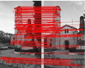
The next step is to use these potentially matching corners to compute the fundamental matrix. This process must be ro-bust, since it can not be assumed that all of the matches are correct. Robustness is achieved by using concepts from the field of robust statistics, in particular, random sampling. Random sampling is a “generate and test process” in which a minimal set of correspondences, in this case the smallest number necessary to define a unique fundamental matrix (7 points), are randomly chosen (Rousseeuw, 1984, Bolles and Fischler, 1981, Roth and Levine, 1993, Torr and Mur-ray, 1993, Xu and Zhang, 1996). A fundamental matrix is then computed from this best minimal set. The set of all corners that satisfy this fundamental matrix is called the support set. The fundamental matrixFij, with the largest
support setSFijis returned by the random sampling
pro-cess. The matching corners (support set) for two typical wide baseline views is shown in Figure 1.
Figure 1: The matching corners for two views 6 TRILINEAR TENSORS
While this fundamental matrix has a high probability of being correct, it is not necessarily the case that every corre-spondence that supports the matrix is valid. This is because the fundamental matrix encodes only the epipolar geome-try between two images. A pair of corners may support the correct epipolar geometry by accident. This can occur, for example, with a checkerboard pattern when the epipo-lar lines are aligned with the checkerboard squares. In this case, the correctly matching corners can not be found using only epipolar lines (i.e. computing only the fundamental matrix). This type of ambiguity can only be dealt with by computing the trilinear tensor.
Assume that we see the point X = [X, Y, Z]T
, in three camera views, and that 2D co-ordinates of its projections are ˜u= [u, v, 1]T, ˜u′ = [u′, v′, 1]T, ˜u′′= [u′′, v′′, 1]T. In
addition, in a slight abuse of notation, we define ˜uias the i’th element of u; ie. u1= u, and so on. It has been shown
that there is a 27 element quantity called the trilinear tensor T relating the pixel co-ordinates of the projection of this 3D point in the three images (Shashua, 1995). Individual elements ofT are labeled Tijk, where the subscripts vary in
the range of 1 to 3. If the three 2D co-ordinates(˜u, ˜u′, ˜u′′)
truly correspond to the same 3D point, then the following four trilinear constraints hold:
u′′T
i13˜ui− u′′u′Ti33˜ui+ u′Ti31u˜i− Ti11˜ui= 0
v′′T
i13u˜i− v′′u′Ti33˜ui+ u′Ti32u˜i− Ti12˜ui= 0
u′′T
i23u˜i− u′′v′Ti33˜ui+ v′Ti31u˜i− Ti21˜ui= 0
v′′T
i23˜ui− v′′v′Ti33˜ui+ v′Ti32u˜i− Ti22˜ui= 0
In each of these four equationsi ranges from 1 to 3, so that each element of ˜u is referenced. The trilinear tensor was previously known only in the context of Euclidean line correspondences (Spetsakis and Aloimonos, 1990). Gen-eralization to projective space is relatively recent (Hartley, 1995, Shashua, 1995).
The estimate of the tensor is more numerically stable than the fundamental matrix, since it relates quantities over three
views, and not two. Computing the tensor from its corre-spondences is equivalent to computing a projective recon-struction of the camera position and of the corresponding points in 3D projective space.
6.1 Computing the Trilinear Tensor
We compute the trilinear tensor from the correspondences that form the support set of two adjacent fundamental ma-trices in the image sequence. Previously we computed the fundamental matrix for every pair of images. Now we fil-ter out those image pairs that do not have more than a cer-tain number of supporting matches. This leaves a subset of thesen2
image pairs that have valid fundamental matri-ces. Consider three images,i, j and k and their associated fundamental matricesFijandFjk. Assume that these
fun-damental matrices have a large enough set of supporting correspondences, which we callSFijandSFjk. Say a
par-ticular element ofSFij is(xi, yi, xj, yj) and similarly an
element ofSFjkis(x′j, yj′, x′k, y′k). Now if these two
sup-porting correspondences overlap, that is if(xj, yj) equals
(x′
j, y′j) then the triple created by concatenating them is a
member ofCTijk, the possible support set of tensorTijk.
The set of all such possible supporting triples is the input to the random sampling process that computes the tensor. The result is the tensorTijk, and a set of triples (corner in
the three images) that actually support this tensor, which we callSTijk.
A tensor is computed for every possible triple of images. In theory this isO(n3
), but in practice it is much less. The reason is that only a fraction (usually from10 to 30 per-cent) of the n2
possible fundamental matrices are valid. And from this fraction, an even smaller fraction of the pos-sible triples are valid.
7 CHAIN THE CORRESPONDENCES
The result of this process is a set of trilinear tensors for three images along with their supporting correspondences. Say that we have a sequence of images numbered from 1 to n. Assume the tensors Tijk andTjkl have
support-ing correspondences (xi, yi, xj, yj, xk, yk) in STijk and
(x′
j, y′j, x′k, yk′, x′l, yl′) in STjkl. Those correspondences
for which(xj, yj, xk, yk) equals (xj′, y′j, x′k, y′k) represent
the same corner in imagesi, j, k and l. In such cases we say that this corner identified inTijkis continued byTjkl.
The goal of this step is to compute the maximal chains of supporting correspondences for a tensor sequence. This is done in a breadth first search using the supporting tensor correspondences as input. Individual correspondences that are continued by a given tensor are chained for as long as is possible. The output of the process is a unique identi-fier for a 3D corner, and its chain of 2D feature correspon-dences in a sequence of images. This corner list is then sent directly to the commercial bundle adjustment program Photomodeler (Photomodeler by EOS Systems Inc., n.d.) using a Visual Basic routine that communicates through a DDE interface.
8 AUTOCALIBRATION OF FOCAL LENGTH
To run the bundle adjustment it is necessary to know the camera calibration. However, it was not necessary to know the camera calibration to compute these correspondences. As a side effect of computing these correspondences we have a set of fundamental matrices between input images. It is possible to autocalibrate the camera parameters from these fundamental matrices.
The goal of autocalibration is to find the intrinsic camera parameters directly from an image sequence without re-sorting to a formal calibration process.
The standard linear camera calibration matrixK has the following entries (Hartley, 1997b):
C = f ku 0 u0 0 f kv v0 0 0 1 ! (1) This assumes that the camera skew isπ/2. Here f is the focal length in millimeters, andku, kvthe number of
pix-els per millimeter. The termsf ku, f kv can be written as
αu, αv, the focal length in pixels on each image axis. The
ratioαu/αvis the aspect ratio. It is often the case that all
the camera parameters are known, except the focal length f . The reason is that many digital cameras have a zoom lens, and thus can change their focal length. The other camera parameters are specified by the camera manufac-turer.
Thus a reasonable goal of autocalibration process is simply to find the focal length. This can be done reliably from the fundamental matrices that have been computed as part of the procedure to find the correspondences between image pairs (Roth, 2002).
8.1 Autocalibration by Equal Singular Values
If we know the camera calibration matrixK, then the es-sential matrixE is related to the fundamental matrix by E = CtF C. The matrix E is the calibrated version of
F; from it we can find the camera positions in Euclidean space. Since F is a rank two matrix, E also has rank two. However,E has the extra condition that the two non-zero singular values must be equal. This fact can be used for autocalibration by finding the calibration matrixC that makes the two singular values of F as close to equal as possible (Mendonca and Cipolla, 1999). Given two non zero singular values of E: σ1 andσ2 (σ1 > σ2), then,
in the ideal case(σ1− σ2) should be zero. Consider the
difference(1 − σ2/σ1). If the singular values are equal
this quantity is zero. As they become more different, the quantity approaches one. Given a fundamental matrix, au-tocalibration proceeds by finding the calibration matrixK which minimizes(1 − σ2/σ1).
Assume we are given a sequence ofn images, along with their fundamental matrices. ThenFi, the fundamental
ma-trix relating imagesi and i + 1, has non zero singular val-ues σi1 and σi2. To autocalibrate from these n images
using the equal singular values method we must find the K which minimizes Pn−1
i=1 wi(1 − σi2/σi1). Here wi is
a weight factor, which defines the confidence in a given fundamental matrix. The weightwiis set in proportion to
the number of matching 2D feature points that support the fundamental matrixFi. The larger this number, the more
confidence we have in that fundamental matrix. In the case where only the focal length needs to be autocalibrated the minimization of this quantity is a simple one dimensional optimization process.
9 EXPERIMENTS
There are as yet no standardized data sets for testing wide baseline matching algorithms. However, there is one data set that has been used in a number of wide baseline match-ing papers (Schaffalitzky and Zisserman, 2002, Ferrari et al., 2003, Martinec and Pajdla, 2002), which is the Val-bonne church sequence as shown in Figure 2.
Figure 2: Twelve pictures of the Valbonne Sequence This sequence has a number of views of the church at Val-bonne, in France. These views are typical of what would be used in a photogrammetric model building process. This sequence was processed by our software. There were ap-proximately 350 feature points over these twelve images, and each feature point exists in at least five or more im-ages. There are twelve images, so one would expect122
fundamental matrices, and about123
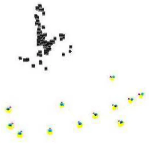
trilinear tensors to be calculated. However, only about fifty percent of the max-imum number of fundamental matrices is calculated, and likewise, only thirty percent of the maximum number of trilinear tensors. A rendering of the camera positions and feature points is shown in Figure 3. The RMS residual er-ror of each feature point when it is reprojected into the 2D image is at most 0.8 pixels, and at least 0.1 pixels. Thus
we can see that the feature points are computed reliable enough to produce a good 3D reconstruction. The autocal-ibrated focal length of the camera is610.00 pixels, while the true focal length is listed as685 pixels, which is within about15 percent of the correct value.
Figure 3: Rendering of camera positions and feature points 10 DISCUSSION
In this paper we have described a system which automati-cally computes the correspondences for an unordered set of overlapping images. These correspondences are then sent to a bundle adjustment process to compute the extrinsic camera parameters. This process does not require camera calibration, and in fact can autocalibrate the camera focal length. A demonstration version of this code can be found in http://www.cv.iit.nrc.ca/research/PVT.html.
REFERENCES
Baumberg, A., 2000. Wide-baseline muliple-view correspon-dences. In: Proc. IEEE Conference on Computer Vision and Pat-tern Recognition, Hilton Head, South Carolina, pp. 1774–1781. Bolles, R. C. and Fischler, M. A., 1981. A ransac-based approach to model fitting and its application to finding cylinders in range data. In: Seventh International Joint Conference on Artificial Intelligence, Vancouver, British Colombia, Canada, pp. 637–643. Ferrari, V., Tuytelaars, T. and Gool, L. V., 2003. Wide-baseline muliple-view correspondences. In: Proc. IEEE Conference on Computer Vision and Pattern Recognition, Madison, Wisconsin, pp. 348–353.
Harris, C. and Stephens, M., 1988. A combined corner and edge detector. In: Proceedings of the 4th lvey Vision Conference, pp. 147–151.
Hartley, R., 1995. A linear method for reconstruction from lines and points. In: Proceedings of the International Conference on Computer Vision, Cambridge, Mass., pp. 882–887.
Hartley, R., 1997a. In defence of the 8 point algorithm. In: IEEE Transactions on Pattern Analysis and Machine Intelligence, Vol. 19number 6.
Hartley, R., 1997b. Kruppa’s equations derived from the funda-mental matrix. IEEE Trans. on Pattern Analysis and Machine Intelligence 19(2), pp. 133–135.
Longuet-Higgins, H., 1981. A computer algorithm for recon-structing a scene from two projections. Nature 293, pp. 133–135. Lowe, D., 1999. Object recognition from scale invariant features. In: International Conference on Computer Vision, IEEE Com-puter Society, pp. 1150–1157.
Martinec, D. and Pajdla, T., 2002. Structure from many per-spective images with occlusions. In: Computer Vision - ECCV 2002, 7th European Conference on Computer Vision, Copen-hagen, Denmark, May 28-31, 2002, Proceedings, Part II, Lecture Notes in Computer Science, Vol. 2351, Springer, pp. 355–369. Mendonca, P. and Cipolla, R., 1999. A simple technique for self-calibration. In: Proceedings of IEEE Conference on Computer Vision and Pattern Recognition, Fort Collins, Colorado, pp. 112– 116.
Mikolajczk, K. and Schmid, C., 2003. A performance evaluation of local descriptors. In: Proc. IEEE Conference on Computer Vision and Pattern Recognition.
Photomodeler by EOS Systems Inc., n.d. http:/www,photomodeler.com.
Pritchett, P. and Zisserman, A., 1998. Wide baseline stereo matching. In: Proc. International Conference on Computer Vi-sion, Bombay, India.
Roth, G., 2002. Some improvements on two autocalibratio algo-rithms based on the fundamental matrix. In: International Con-ference on Pattern Recognition: Pattern Recognition Systems and Applications, Quebec City, Canada.
Roth, G. and Levine, M. D., 1993. Extracting geometric primi-tives. Computer Vision, Graphics and Image Processing: Image Understanding 58(1), pp. 1–22.
Roth, G. and Whitehead, A., 2000. Using projective vision to find camera positions in an image seqeuence. In: Vision Interface 2000, Montreal, Canada, pp. 87–94.
Rousseeuw, P. J., 1984. Least median of squares regression. Jour-nal of American Statistical Association 79(388), pp. 871–880. Schaffalitzky, F. and Zisserman, A., 2002. Multi-view matching for unordered image sets. In: Proceedings of the 7th European Conference on Computer Vision, Copenhagen,Denmark. Shashua, A., 1995. Algebraic functions for recognition. IEEE Transactions on Pattern Analysis and Machine Intelligence 17(8), pp. 779–789.
Spetsakis, M. and Aloimonos, J., 1990. Structure from motion using line correspondences. International Journal of Computer Vision 4(3), pp. 171–183.
Torr, P. and Murray, D., 1993. Outlier detection and motion seg-mentation. In: Sensor Fusion VI, Vol. 2059, pp. 432–443. Xu, G. and Zhang, Z., 1996. Epipolar geometry in stereo, motion and object recognition. Kluwer Academic.