Uncertainty analysis - preliminary data error estimation for ship model experiments

READ THESE TERMS AND CONDITIONS CAREFULLY BEFORE USING THIS WEBSITE. https://nrc-publications.canada.ca/eng/copyright

Vous avez des questions? Nous pouvons vous aider. Pour communiquer directement avec un auteur, consultez la première page de la revue dans laquelle son article a été publié afin de trouver ses coordonnées. Si vous n’arrivez pas à les repérer, communiquez avec nous à [email protected].

Questions? Contact the NRC Publications Archive team at

[email protected]. If you wish to email the authors directly, please see the first page of the publication for their contact information.

Archives des publications du CNRC

This publication could be one of several versions: author’s original, accepted manuscript or the publisher’s version. / La version de cette publication peut être l’une des suivantes : la version prépublication de l’auteur, la version acceptée du manuscrit ou la version de l’éditeur.

Access and use of this website and the material on it are subject to the Terms and Conditions set forth at

Uncertainty analysis - preliminary data error estimation for ship model

experiments

Hermanski, G.; Derradji-Aouat, A.; Hackett, P. J.

https://publications-cnrc.canada.ca/fra/droits

L’accès à ce site Web et l’utilisation de son contenu sont assujettis aux conditions présentées dans le site LISEZ CES CONDITIONS ATTENTIVEMENT AVANT D’UTILISER CE SITE WEB.

NRC Publications Record / Notice d'Archives des publications de CNRC:

https://nrc-publications.canada.ca/eng/view/object/?id=2668d3c0-06b2-4066-aae1-78d3e71c09f1 https://publications-cnrc.canada.ca/fra/voir/objet/?id=2668d3c0-06b2-4066-aae1-78d3e71c09f1

UNCERTAINTY ANALYSIS - PRELIMINARY DATA ERROR ESTIMATION FOR SHIP

MODEL EXPERIMENTS

Greg Hermanski, Ahmed Derradji-Aouat and Peter Hackett

National Research Council of Canada, Institute for Marine Dynamics, St. John’s, NF, A1B 3T5, Canada.

ABSTRACT

Experimental Uncertainty Analysis (EUA) is a process “as well as a practice” that needs to be followed to estimate the level of confidence (or the level of uncertainty) in experimental results. Through this process, a scientist or an engineer can quantify the agreement “the closeness or difference” between the results obtained in a given experiment and their “true” values.

Experiments to measure ship motions, wave impact forces, and pressures were performed at the Institute for Marine Dynamics (IMD) of the National Research Council of Canada (NRC). The experiments were conducted in calm water, and in regular and irregular waves. A self-propelled ship-model was tested at various ship speeds and headings. The experimental results will be used as a database to benchmark computer codes and validate numerical research work currently underway at the IMD and DREA (Defense Research Establishment Atlantic).

Uncertainty Analysis (UA) was performed on the results of the ship experiments. The objective is to quantify the level of uncertainty in the measured data. Both systematic (fixed) and random (precision) uncertainties associated with the measured ship motions, wave impact forces, and pressures were calculated. Potential uncertainty “error” sources were identified, and all significant elemental uncertainties were calculated. Both systematic and random uncertainties were added to compute the overall uncertainty. A discussion is presented regarding the effects and the contributions of various sources to the overall uncertainty as well as the propagation of the elemental uncertainties throughout all stages of the experimental program. Conclusions are reported and recommendations for future work are indicated.

INTRODUCTION

Uncertainty Analysis is a process “as well as a practice” that needs to be followed to estimate the level of confidence (or the level of uncertainty) in given experimental results. Through this process, experimentalists are able to quantify the agreement between the measured results and their true values.

Uncertainty analysis is a process that needs to be followed during all stages of any experimental research program, starting from the program’s planning stage, through the design and instrumentation, installation and test set-up, actual testing, data acquisition and data reduction analysis, to reporting (Coleman and Steele, 1998, 2001). General uncertainty analysis is performed during the planning stage. It can

result in the identification of major sources for errors, and it justifies the need for their improvements to enhance accuracy. It can optimize the overall project cost for the required accuracy. Also, it provides essential information that guarantee acceptable (or required) levels of accuracy in the experimental results.

Experimentalist Kline (1985) defined Uncertainty Analysis as:

Uncertainty analysis is an essential ingredient in planning, controlling and reporting experiments. The important thing is that a reasonable uncertainty analysis be done. It is particularly important to use an uncertainty analysis in the planning and checkout stages of an experiment. Uncertainty analysis is the heart of quality control in experimental work.

Historically, experimental uncertainty analysis (EUA) was not, extensively, used in hydrodynamic testing until the late 1980's. The International Towing Tank Conference (ITTC) and the International Ship and Offshore Structure Congress (ISSC) have recommended the application of uncertainty analysis in both experimental and computational fields. The ITTC validation panel, established by the 18th ITTC, presented its recommendations to the 19th ITTC. The 22nd ITTC (1999) issued a Quality Manual that includes uncertainty analysis guidelines for both EFD (Experimental Fluid Dynamics) and CFD (Computational Fluid Dynamics). The ITTC guidelines were based on the work by Coleman and Steele (1989) and the 1995 AIAA standards (American Institute for Aeronautics and Astronautics). The ISSC (2000) called for a broader application of uncertainty analysis in both experimental (EUA) and numerical (NUA) fields. Also, it called the development of a qualitative criterion for validation of numerical codes.

The field of Numerical Uncertainty Analysis (NUA) is in its infancy stage (Coleman and Steele, 2001). Research in the V&V field (verification and validation analysis) is growing. Today, Coleman and Stern (1997 and 1998) are the pioneers in the fields CFD code validation and numerical uncertainty calculations.

Experiments to measure ship motions, wave impact forces, and pressures distribution over the hull were performed at the Institute for Marine Dynamics (IMD) of the National Research Council of Canada (NRC). The experiments were conducted in calm waters, and in regular and irregular waves.

Experiments in calm water and regular waves were conducted in the Clear Water Tank (CWT), while experiments in irregular waves conditions were conducted in both CWT and the Offshore Engineering Basin (OEB)

A self-propelled ship model was tested at various ship speeds and headings. The experimental results will be used as a database to benchmark computer codes and validate numerical research work currently underway at the IMD and DREA (Defense Research Establishment Atlantic).

In this study, the main findings of an uncertainty analysis on the results of the ship model experiments are reported. The objective is to provide a qualitative analysis that can be used to serve as an initial a yardstick to quantify the level of uncertainty in the measurements (with the required level of confidence).

In this paper, both systematic (fixed or bias) and random (precision) uncertainties associated with the measurements of the ship model motions, wave impact forces, and pressures are calculated. Potential systematic error sources in the experimental set-up were identified, and uncertainties induced by each “elemental source” are calculated. All bias elemental uncertainties are added to calculate the overall bias error. The random uncertainty (repeatability error) is calculated for each channel, during each test run. The total uncertainty is taken as the sum of both systematic and random uncertainties.

The effects and the contributions of various elemental sources to the overall uncertainty are discussed. Propagations of uncertainties throughout all stages of the experiments are pointed out. Conclusions are reported and recommendations are suggested.

EXPERIMENTAL PROGRAM

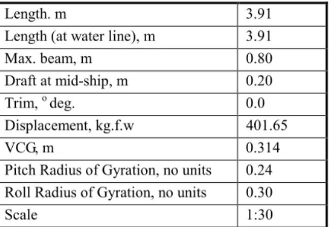
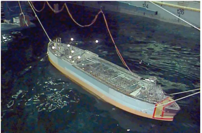
The 1:30 model of a concept design of the twin screw, twin rudder, icebreaking, passenger ferry was used to conduct the experiments (Fig. 1). The model was designed and instrumented to measure rigid body motions, bow relative motions, three component forces (due to wave impact on the bow visor) and pressure distribution over the hull (below the water line). The model specifications and hydrostatics are given in Table 1.

Experiments were performed at various speeds and headings. For experiments in the CWT, the model was hard wired to the carriage (the driver of the model controlled the propellers revolutions and the rudder angle from the carriage). In the OEB, however, the model was driven by an autopilot for pre-set propeller revolutions and headings (the model control was wireless).

Table 1: Hull Geometry and Hydrostatics

Length. m 3.91

Length (at water line), m 3.91

Max. beam, m 0.80

Draft at mid-ship, m 0.20

Trim, o deg. 0.0

Displacement, kg.f.w 401.65

VCG, m 0.314

Pitch Radius of Gyration, no units 0.24 Roll Radius of Gyration, no units 0.30

Scale 1:30 During each test, the data was collected and

stored in a computer system on board of the ship model, and after each test run, the data was transmitted to a permanent storage disk.

A total of over 500 test runs were carried out in both the CWT and in the OEB. For the purpose of this analysis, only 54 test runs are presented. These are: • 24 test runs in calm water. The test runs were

carried out (in the CWT) at three different speeds: 8 knots (4 runs), 10 knots (4 runs), and 14 knots (16 runs).

• 3 test runs in regular waves. The tests were conducted (in the CWT) at three speeds (8, 10, and 14 knots – same speeds as in the calm water test runs) for the following wave conditions: Lw/Ls = 1.4 (wave length/ship length) and wave slope of 1/25.

• 27 test runs for irregular waves. The test runs were carried out in CWT (7 runs) and OEB (20 runs). The ITTC spectrum with Hs = 8m and Tp = 13.5 sec was selected. The tests were conducted in head seas (heading of 180o) in the CWT (7 runs) and in oblique seas in the OEB (10 runs for the 150o heading and an-other 10 runs for the 120o heading).

This selection of these tests was deemed to be necessary since it is not possible to analyze all of the 500 test runs for this study. Table 2 shows the matrix of all tests reported in this paper.

For each “selected test”, the output from only 12 channels were analyzed. It was decided that it is not practical to analyze the output from all 40

channels. Thus, the present analysis is focussed only on the following parameters (channels):

• Ship speed (channel 1)

• Model pitch and roll angles and heave acceleration (channels 17, 18, and 19, respectively).

• Visor forces in all three directions (channels 10, 11, and 12)

• Propeller shaft speed (channel 24).

• Pressures at four locations (channels 27, 29, 37, and 36)

The location of the load cells used to measure the visor forces and the locations of the pressures sensors are shown in Fig. 2 (the figure shows, also, the coordinate system).

For clarity, it should be pointed out that the present study is confined to uncertainty analysis of the output of each channel in each test. Further uncertainty analysis work is needed when the results of the experiments are presented using any data reduction equations (DRE) and/or curve fitting regressions, such as the relationship between the ship model speed and the normalised visor forces.

Table 2: Test Matrix

Test Type V (Note 1) Heading

(Note 2) Calm_Water 14, 10, 8 180 REG_Waves 14, 10, 8 180 IRREG_Waves (ITTC Spectrum) 14 150, 120, 180

Note 1: V = Ship speed (full scale)

Note 2: 180O heading = head sea, model moving towards the waves.

UNCERTAINTY ANALYSIS – THE CONCEPT

Uncertainty in any given measurement is defined as the possible maximum error that may be involved in that measurement. The uncertainty (Ux) in

a measured value of (X) may be expressed as: X U best X true X = ± (1)

where Xtrue is the true value of X, Xbest is the best

estimate (either the best value that can be obtained in a single sample measurement or the mean value of N readings in multi-sample measurements).

In any measurement, the total uncertainty (U) is defined as the sum of the systematic component (B) and the random component (P). Coleman and Steele (1998) formulated U as:

(

B

P

)

U

2 2

+

±

=

(2) In the literature, the systematic uncertainty is also known as the fixed error or the bias error. The random uncertainty, however, is known as the repeatability error or the precision uncertainty. The magnitudes of systematic uncertainties do not change from test to test for a given experimental setup. Systematic uncertainties are mainly attributed to instrument calibrations, their installation, and uncertainties in the data conditioning and processing systems.

The random uncertainties are statistical in nature, and they are directly dependent on the effects of the environmental conditions of the test run and the particulars of test setup.

In practice, systematic uncertainties (B’s) can be minimized by the calibration processes of the instrument, but only to the limit set by the quality of the calibration process and the manufacturer’s specifications. It should be pointed out that, in most cases, it is extremely difficult to calculate bias uncertainties, and therefore, they are estimated using engineering judgements based on previous experience. Statistical methods for random error estimates are applicable to the calculations of precision uncertainties. Precision error distribution is characterized by a normal probability density distribution. Theoretically, in an infinite sample population, all observations should follow a two-tailed Gaussian distribution curve, and the precision error in the mean value of the population is zero. However, since sample population is always finite, all measurements from any test program can be viewed as a subset of the larger parent Gaussian distribution, and

the precision error is estimated based on size of population and its standard deviation for a chosen confidence level. Usually, in engineering, the 95 % confidence level is used.

The sum of both systematic and random uncertainties is called total or “overall” uncertainty. Figure 3 shows a schematic for the concept of both systematic and random uncertainties.

Figure 1a: Ship Model in the CWT

Figure 1b: Ship Model in the OEB Uncertainty Analysis – Equations

During an experiment, some variables are measured directly. In many cases, the final experimental results are calculated using Data Reduction Equations (DRE). For example, if R is a result that is function of the measured variables Xj

)

...,

,

,

(

R

=

R

X

₁

X

₂

X

_j (3) The uncertainty involved in using the DRE to calculate the result R is UR:

              ∂ ∂       ∂ ∂       ∂ ∂ Xj U Xj R 2 + ... X2 U X2 R 2 + X1 U X1 R 2 2 1 = R U (4)

where UXj (j = 1, 2, 3, …) are the uncertainties

associated with each variable Xj and ∂R/∂Xj ( j= 1, 2,

3, ..) are partial derivatives of the function R with respect to the measured variable X, (also, they are called sensitivity coefficients).

Equation (4) is based on a Taylor series expansion of the DRE, with the assumption that all non-linear terms in the series are either zero or small enough to be ignored. And, both the function R and its derivatives are continuous in the domain of interest.

Figure 2: Locations of the three component load cell and pressure transducers.

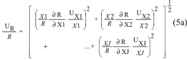
If both sides of Eq. 4 are divided by the result R, and each term on the right hand side of the equation is multiplied by Xj / Xj, (where j= 1, 2 , 3, ..etc.)1 , thus:

1 _{The ratio Xj/Xj is equal to unity (Xj/Xj = 1),}

                          ∂ ∂ +         ∂ ∂         ∂ ∂ XJ U XJ R 2 + ... 2 X2 U X2 R 2 2 + 1 X1 U X1 R 1 2 2 1 = R U XJ R XJ X R X X R X R (5a)

Equation 5a is a non-dimensional form of Eq. 4. It is used to calculate the relative uncertainty induced by each variable in the result R. The ratios UXj/Xj are

the relative uncertainties induced by the variable Xj. Their multiplying factors are called the uncertainty magnification factors (UMF):

Xj R = UMF ∂ ∂ R Xj _(5b)

Therefore, Eq. 5a becomes:

                                              U Xj U MFj 2 + ... 2 X2 U MF2 2 + 1 X1 U MF1 2 2 1 = R Xj U X U X U R (5c)

For a given variable, Xj, a UMF value greater than 1 indicates that the uncertainty Uxj is magnified. If the UMF value for Xj is less than 1, thus, the uncertainty in the Uxj diminishes as it propagates through the DRE.

Figure 3: Schematic for uncertainties.

Total error, U. Bias error, B True Value Measured Value Precision error, P

.

Average Measurement (µ Scatter due to precision error

Pressure Transducers

3 Component

Load Cell

Z

Y

X

Alternatively, if both sides of Eq. 4 can be divided by UR, thus: .... U U X2 R U U X1 R 1 2 R X2 2 R X1

=

+             ∂ ∂             ∂ ∂

+

(6a)

The uncertainty percentage contribution (UPC) is defined as: 100 * R U Xj U Xj R 2 = UPC       ∂ ∂ (6b)

The UPC gives an estimate of the percentile contributed by each source to the overall uncertainty.

In special cases, where the DRE is expressed in the following format:

.... c 3 X b 2 X a 1 X * k R = (6c)

the relative uncertainty equation (Eq. 5c) for the result R takes the following form:

                                                  j X Xj U 2 2 c + 2 X X2 U 2 2 b + 1 X X1 U 2 2 a = 2 R R U _(6d)

where k, a, b, and c are constants, Xj ( j =1, 2, 3, …)

are measured variables. Note that the signs of the exponents (a, b, and c) have no effect on the numerical value of the calculated uncertainty (since all exponents are squared). In Eq. 6c, uncertainty values are magnified by exponents greater than 1, and they are reduced if the exponent value is less than 1.

Random Uncertainty Formulation

The random uncertainty P associated with a sample population of N readings is calculated using one of the following equations:

S

*

t

P

xi

=

xi (7a)

N

S

*

t

P

xi Ni

=

(7b)

where: t is a coefficient obtained from the t distribution table (given by Coleman and Steele, 1998), and Sx is the standard deviations of the sample population, and N is an integer for the multi-sample tests 2 N 1 I i X X X 1 -N 1 S       ∑       −       = = − (8a) where X is the mean values of all measured variables Xi.

∑

=

=

N i

Xi

N

X

1

1

(8b)

Conceptually, Eq. 7a is used in the case of a single experiment, where the entire test run is divided into N segments. The result of each segment is taken as one data point. Thus, from a single test, N data points are obtained (although the test is not independently repeated).

Alternatively, Eq. 7b is used in multiple test experiments, where a test is independently repeated N times. The result of each test is taken as one data point. Thus, N data points are obtained from the results of N independent tests.

Random uncertainty propagation for a variable can estimated as:

[

(

P

)

+

(

P

)

+

...

+

(

P

)

]

=

P

i 2M 2 2 i 2 1 i 2 1 i (9)

where (Pi)M (M = 1, 2, 3…) is the elemental error

source. Once the elemental precision limit for each variable is established, the precision limit for the entire experiment is calculated using Eq. 4.

Systematic Uncertainty Formulation

Three major sources of the systematic error are readily identified. These are the calibration process, the data acquisition, and the data reduction.

Regardless of the source, all elemental systematic uncertainties have to be estimated, and the following equation is used to calculate the overall bias uncertainty value of a given variable.

[

(

B

)

+

(

B

)

+

...

+

(

B

)

]

=

B

i 2M 2 2 2 1 i 2 1 i (10a)

Once all systematic uncertainties for all variables are established, the overall bias uncertainty for the entire experimental result is calculated as:









θ

∑ θ

∑

θ

∑

+ = −

B

2

+

B

=

B

k ik J 1 i k i 1 J 1 = k 2 i 2 i 2 1 J 1 = i R (10b)

where θi,k are sensitivity coefficients, and Bi,k

are the elemental systemetic uncertainties.

Eq. 10b is general in nature, and it is applicable to the analysis of any test results. The double sum on the right hand side of the equation reflects correlation between variables. For situations where there are no correlations between variables, the correlation term is zero, and Eq. 10b becomes similar to Eq.4.

UNCERTAINTY CALCULATIONS

In this section, calculations of systematic, random, and total uncertainties are presented. The

details regarding errors induced by instruments calibrations and installations (such as transducers and the load cell) are given in Appendix A

Bias Uncertainties:

Table 3a shows an example for the calculation of systematic uncertainties. The example shows contributions of the transducer and the 16-channel conditioner of the Data Acquisition System (DAS) used in the measurement of the visor force in the X direction (Fx).

During the initial stage of this analysis, all possible sources for bias errors were identified and bias uncertainty values (B) associated with each source were calculated. The significant sources are

reported in Table 3b. In this study, a significant uncertainty source is defined as any source that produces an uncertainty value ≥ 5% of the value given by the largest source (the most significant contributor).

Using the manufacturer’s specification data sheets, the majority of the systematic uncertainty values were calculated. In this test program, the most significant sources for bias uncertainty are attributed to the transducers and DAS. Note that, in this study, all values used in the uncertainty calculations are those specified for worst cases (not “typical”).

All bias uncertainty values are expressed in terms of percent of full scale. In cases where the manufacturer did not have specifications to cover the whole range in which a DAS channel is configured, the specifications were extended to provide a conservative “over estimate” of the bias error value. For example, suppose that a manufacturer specification data sheet references a bias error contributor at a gain of 1000 (volt/volt), whereas during the experiment, gains of up to 3000 (volt/volt) were utilized. In this analysis, the resultant bias error for a gain of 1000 (volt/volt) is multiplied by 3. This reflects the contribution at the gain of 3000 (volt/volt).

Throughout the calculations of bias uncertainties of the transducers and DAS, a temperature change of 10oC is used to account for the difference between the calibration and operational temperatures. That is the difference between the temperature at the time of bench calibrations and the steady state temperature of the equipment installed in the model.

Random Uncertainties

In order to calculate random uncertainties in a given experimental measurement, an end-to-end

approach was followed. The random uncertainty of measured data was evaluated from the precision of repeated measurements of the same set point.

In general, random uncertainty analysis deals with uncertainties induced by noise in instrumentation as well as uncertainties in the test results itself. Uncertainties induced by instrumentation noise include transducers’ noise (such as thermal noise and

motor brush noise) as well as noise induced by the DAS (such as noise in the signal-conditioning amplifier and in the signal conditioning excitation).

Uncertainties induced by instrumentation noise are, usually (but not always), negligible. In this paper, they are calculated and reported in Tables 4 to 6.

Random uncertainties in the measured results are calculated using either Eq. 7a or Eq. 7b.

In order to calculate uncertainties in the measured data, two sets of parameters were needed: The first set includes:

a) Mean values of the output from each of the 12 channels

b) Standard deviation of the mean values (mean values for the output of each channel)

c) Mean value of the means (mean value of the mean values of the output from each channel),

The second set of parameters includes:

d) Standard deviation of the output from each channel

e) Standard deviation of the standard deviations of the output of each channel

f) Double amplitude (peak to peak) of the output response in waves

It was assumed that the first set of parameters is needed in the analysis of all experiments, while the second set of parameters is needed only in experiments in waves.

Conceptually, the standard deviation of the means (b) is used to investigate possible variation in the repeatability of means, while the standard deviation of the standard deviations (e) is used to investigate possible variation in the repeatability of standard deviations. Note that standard deviation values (d) are, also, used to calculate amplitudes of dynamic responses for experiments in waves.

In principle, the repeatability of means (using parameter b) indicates uncertainty in the static response, while the repeatability of standard deviations (using parameter e) indicates uncertainty in the dynamic response.

Since uncertainty values need to be specified (and reported) in percentile, the calculated values are

divided by the calibration range (for the case of repeatability of means). Also, they are divided by the double amplitude response (for the case of repeatability of standard deviations).

The calculated random uncertainties (for all tests) are given in Tables 4, 5, and 6. An analysis of the results in the tables (4, 5, and 6) revealed the following:

Calm Water Tests - Random Uncertainties For the calm water tests, precision uncertainty values were calculated using the multiple sample test technique (Eq. 7b). All tests were, independently, repeated several times. They were repeated sixteen times for experiments at ship speed of 14 knots (N = 16), repeated 4 times for experiments at ship speed of 10 knots (N = 4), and repeated 4 times for experiments at ship speed of 8 knots (N = 4). For the 95% confidence interval coverage, t = 2.000 for the 15 degrees of freedom (DOF), and t = 3.182 for the 3 DOF (In EUA, DOF = N – 1).

The value of Sx (in Eq. 7b) is taken as the standard deviation of mean values.

Table 4a shows an example of how the random uncertainties are calculated for calm water experiments (the example is for ship speed of 14 knots). For each channel, the mean value, the standard deviation of means, and the mean of means are calculated. Then, the precision uncertainty, P, is calculated using Eq. 7b, with t = 2.000 (N > 10), Sx = standard deviation of the means (parameter b), and N = 16.

Random uncertainties for the other two tests (ship speeds of 8 and 10 knots) were calculated in the same manner as in the case of the 14 knot tests (using Eq. 7b, where t = 3.182 and N = 4 for both tests). Regular Wave Tests - Random Uncertainties

Precision uncertainties for regular wave experiments were estimated using Eq. 7a (this is the case of a single sample test measurement). Test runs were not repeated. For the analysis, the time series of each test run is divided into 10 equal segments, each segment consists of four or five full response cycles.

Two values for Sx (in Eq. 7a) are calculated, These are the standard deviation of the means (for the repeatability of means) and the standard deviation of the standard deviations (for the repeatability of standard deviations). For the 95% confidence coverage, t = 2.00 (N

≥

10).

Table 5a gives an example of random uncertainty calculations for the results of an experiment in regular waves (the example is for ship speed of 8 knots). Precision uncertainty, P, is calculated for two different cases:

P = 2 * standard deviation of the means (to investigate repeatability of means)

P = 2 * standard deviation of the standard deviations (to investigate repeatability of standard deviations)

In Table 5a, both values of P are given for each channel. It is hypothesised that the mean value is used to indicate precision uncertainty in static response, while the second value is used to indicate precision uncertainty in dynamic response.

The same analysis steps were taken for the results of the other two experiments “10 and 14 knots”. Table 5b gives a summary for all precision uncertainties calculated for all of the three experiments in regular waves.

Irregular Waves Tests–Random Uncertainties For the irregular waves experiments, precision uncertainty values were calculated using the multiple sample test technique (Eq. 7b). Each test was independently repeated several times. The tests conducted in the OEB were repeated 10 times (heading 150 and 120 degrees) and those carried out in the CWT ware repeated 7 times (heading 180 degrees).

For the 95% confidence coverage, t = 2.000 (N = 10) and t = 2.447 (N = 7).

Similar to the regular wave experiments, two values of Sx are calculated. These are the standard deviation of the means and the standard deviation of the standard deviations.

An example for random uncertainty calculations is given in Table 6a (the example is for heading of 150o). Random uncertainty values, P, were

calculated in the same manner as those in the case of regular wave experiments. Two values for P were calculated from the output of each channel. The first value is used to evaluate repeatability of means (it indicates uncertainty in static response), while the second value is used to evaluate repeatability of the standard deviation (it indicates uncertainty in dynamic response).

Table 6b shows a summary of all tests in irregular waves (all three headings). Two values for P are provided for each channel of each test.

Total Uncertainties:

Table 7 shows the summary for total uncertainties (U) calculated for each channel of each test. Total uncertainties are calculated (using Eq. 2) combining both systematic uncertainties (B) and precision uncertainties (P).

For regular and irregular wave experiments, two values for total uncertainties (U) are calculated. This stems from the fact that, for experiments in waves, two values of random uncertainty (P) were calculated.

The two values of the total uncertainties (Table 7, for experiments in waves) were calculated to report possible variation in the repeatability of means (i.e. uncertainty in the static response) and possible variation in the repeatability of standard deviation values (i.e. uncertainty in the dynamic response).

UNCERTAINTY ANALYSIS – DISCUSSION

In some respect, the present study is only a preliminary uncertainty analysis. It is a rough estimate for maximum potential uncertainties in the experimental results. Every care and every precaution were taken when listing “significant” sources for systematic errors, and in providing realistic estimates for their values. Note that, in this study, most systematic uncertainty values are calculated either using manufacturer’s data/fact sheets or estimated as a result of engineering judgement that is based on previous experience.

The overall study was performed without an outlier analysis. Outliers have the potential to increase

overall uncertainty values. Outlier analysis is a must when the final uncertainty calculation “for any given channel” seems to be larger than expected.

For calm water experiments, maximum total uncertainty of 1.5% in ship motion is calculated. Analysis of the force channels show that maximum total uncertainty of 4.1% is calculated for visor forces, while 14.9% is calculated as the maximum uncertainty value for the pressure channels.

For tests in waves, two (2) values for total uncertainties are provided for each channel. This is due to the fact that two precision uncertainties were calculated from the output of each channel.

In general, for regular wave experiments, total uncertainty values (U) based of the repeatability of standard deviation are larger than those based on the repeatability of the means (Table 7). This indicates that the dynamic response of the model has more uncertainty than its static response.

The results for all three tests, in regular waves, show that maximum value of 9.4% total uncertainty was computed for ship motions. About 8% maximum total uncertainty was computed for visor forces, and 4.6% total uncertainty was obtained from the analysis of the pressure channels (notice the 4.6 % total uncertainty in regular waves experiments is much smaller than the 14.9 % total uncertainty in calm water experiments).

Irregular wave experiments show a more consistent trend with realistic maximum total uncertainty values of 1.6% for ship motions, 1.7% for forces, and 1.9% total uncertainty for pressures.

CONCLUSIONS AND RECOMMENDATIONS

• The majority of the calculated total uncertainties are less than 2%. The 2% total uncertainty values are considered acceptable and satisfactory. • For cases where the total uncertainties are large

(> 2%), the value of U is dominated by the random uncertainty, P, component

• For experiments in irregular waves, both systematic and random uncertainties are comparable.

• The tests carried out in irregular waves have lower random uncertainty than the other two types of tests.

• In the OEB, the ship model was driven by an autopilot (pre-set values for shaft revolutions and heading). In the CWT, a person drove the model. It may well be worth it to investigate the effects of human factors on the calculated uncertainties. • Outlier analysis is not part of this presentation. It

is important to include it any subsequent analyses. • The present study was confined to uncertainty analysis of the output of each channel in each test. Further uncertainty analysis work is needed when the results of the experiments are presented using DRE (and/or curve fitting regressions), such as the relationship between the ship model speed and the normalised visor forces.

REFERENCES

1) Coleman H.W. & Steele W.G. (2001). Experimentation and Uncertainty Analysis.

http://www.uncertainty-analysis.com. An

Uncertainty Analysis course given at the IMD/NRC (Mach., 2001).

2) Coleman H.W. & Steele W.G. (1998). Experimentation and Uncertainty Analysis for Engineers (2nd edition), John Wiley & Sons publications, New York, NY, 1998. Note that the

1st edition of the book had the same title, same authors, and it was published by the same publisher in 1989.

3) Kline, S.J., "The Purpose of Uncertainty Analysis", Journal of Fluids Engineering, Vol.10/153, June 1985.

4) ITTC (1999). Quality Manual, the 22nd International Towing Tank Conference”, Seoul, Korea and Shanghai, China, September 5-11, 1999.

5) AIAA (1995). American Institute for Aeronautics and Astronautics. Assessment of Wind Tunnel Data Uncertainty. Standard S-071-1995.

6) ISSC (2000). Proceedings of the 14th International Ship and Offshore Structures Congress, Nagasaki, Japan, 2-6 October 2000.

7) Coleman H.W. & Stern F. (1997). Uncertainties in CFD Code Validation. ASME Journal of Fluids Eng. Vol. 119, pp. 795-803.

8) Coleman H.W. & Stern F. (1998). Uncertainties in CFD Code Validation - Closure. ASME Journal of Fluids Eng. Vol. 120, pp. 635 – 636.

ACKNOWLEDGMENTS

The authors appreciate the financial support of the NRC/IMD for the uncertainty analysis initiative. Also, they appreciate the discussions with both H. Coleman and G. Steele (2001).

APPENDIX A: BIAS ERRORS DUE TO INSTRUMENTS CALIBRATIONS AND INSTALLATION

The model outfit (instrumentation) included transducers and Data Acquisition System (DAS).

Transducers

• The body angular motions (roll and pitch) were measured directly by Lucas gravity-referenced inclinometers placed at LCG on a deck above VCG and aligned with x and y model axis. The heave acceleration was measured with a Systron Donner MP-1 solid state 6 DOF motion pack placed at model LCG and aligned with z axis • The bow visor 3 component wave impact forces

were measured with AMTI MC3A multi-component force transducer. The load cell was rigidly fixed to a deck at the bow of the model, and the visor was attached to the load cell. • The pressures were measured with Druck and

Endevco piezoresistive pressure transducers. Two 1 psig’s Druck transducers were located on Port and Starboard sides of the bow just below waterline. The Endevco M8510B 15 psig piezoresistive pressure transducers were used to measure pressure on the bow stem line at WL and near the bottom.

Data Acquisition System

The DAS was used to acquire and digitize analog signals from the model, and post process the digitized data. It consists of the following components:

• An NRC designed analog signal conditioning unit.

• An IO Tech Inc. Daqbook /200 Data Acquisition Module.

• An IO Tech Inc. analog multiplexer assembly. • An ICP Inc. Industrial PC Data Acquisition

System Server.

• An ICP Inc. Industrial PC Data Acquisition System Client.

• A Wavelan Wireless Ethernet System.

Calibrations

All transducers were bunch calibrated before they were installed on the model using the model data acquisition system.

Two types of bias error have been identified with respect to the calibration process. Bias errors related to fitting the calibration curve and bias errors related to standards of calibration equipment.

The ship angular motion inclinometers and motion pack were calibrated using standard IMD calibration wedges, with accuracy of ±0.1%. The roll and pitch transducers were calibrated at 2 degrees increments from 0 to 10 degrees range for pitch, and at 5 degrees increments from 0 to 25 degrees range for roll.

The three component load cell was calibrated using standard calibrating weights of ±0.04% accuracy. The calibration range was approximately 250 N for x and y components and 350 N for z component. The calibration was conducted in increments of approximately 50 N and 100 N.

The pressure transducers were calibrated using a Druck Model DPI-600 Portable pneumatic pressure transducer calibrator.

For all transducers, the bias of calibration standards was obtained from:

( )

∑

=

k

1

2

i

W

(ACG)

RC1

B

where ACG is the accuracy of calibration equipment and W is physical values of calibration points (for example 0, 50, 100, 150, 200 and 250 N for load cells)

The calibration data for curve-fitting errors were calculated using the for standard error evaluation method (SEE method):

(

)

∑

−

−

−

=

k i i

N

c

mX

Y

SEE

1 2

2

Where, Yi and Xi are calibration values at ith point, and m and c are slope and intercept of the regression equation. Note that the ±2*SEE band (around the

regression curve) contains about 95% of all data points.

Installations

Installation errors are due to misalignment in installation of instruments with respect to the model axis.

Installation error for the inclinometers and motion pack was evaluated on the basis of the assumption that the accuracy of instruments positioning was ±1 degree with respect to yz and xz planes.

Installation error for the load cell was evaluated assuming that the load cell is fixed with an accuracy of ±1.5 degree with respect to xy and xz planes.

Installation errors for pressure transducers are calculated on the basis of the assumption that the instruments are ±1.5 degree off the normal to the model surface.