Efficient OLAP Operations for RDF Analytics

HAL Id: hal-01101843

https://hal.inria.fr/hal-01101843

Submitted on 9 Jan 2015

HAL is a multi-disciplinary open access

archive for the deposit and dissemination of

sci-entific research documents, whether they are

pub-lished or not. The documents may come from

teaching and research institutions in France or

L’archive ouverte pluridisciplinaire HAL, est

destinée au dépôt et à la diffusion de documents

scientifiques de niveau recherche, publiés ou non,

émanant des établissements d’enseignement et de

recherche français ou étrangers, des laboratoires

Elham Akbari Azirani, François Goasdoué, Ioana Manolescu, Alexandra

Roatis

To cite this version:

Elham Akbari Azirani, François Goasdoué, Ioana Manolescu, Alexandra Roatis. Efficient OLAP

Operations for RDF Analytics. [Research Report] RR-8668, OAK team, Inria Saclay; INRIA. 2015.

�hal-01101843�

0249-6399 ISRN INRIA/RR--8668--FR+ENG

RESEARCH

REPORT

N° 8668

Operations for RDF

Analytics

Elham Akbari Azirani, François Goasdoué, Ioana Manolescu,

Alexandra Roati¸s

RESEARCH CENTRE SACLAY – ÎLE-DE-FRANCE

1 rue Honoré d’Estienne d’Orves Bâtiment Alan Turing

Elham Akbari Azirani, François Goasdoué, Ioana Manolescu,

Alexandra Roatiş

Project-Teams OAK

Research Report n° 8668 — January 2015 — 23 pages

Abstract: RDF is the leading data model for the Semantic Web, and dedicated query languages such as SPARQL 1.1, featuring in particular aggregation, allow extracting information from RDF graphs. A framework for analytical processing of RDF data was introduced in [1], where analytical schemas and analytical queries (cubes) are fully re-designed for heterogeneous, semantic-rich RDF graphs. In this novel analytical setting, we consider the following optimization problem: how to reuse the materialized result of a given analytical query (cube) in order to compute the answer to another analytical query obtained through a typical OLAP operation. We provide view-based rewriting algorithms for these query transformations, and demonstrate experimentally their prac-tical interest.

Sémantique. Des langages de requêtes tels que SPARQL 1.1, permettant en particulier d’exprimer des aggrégations, sont utilisés pour extraire de l’information à partir de graphes RDF.

Dans [1], nous avons défini un modèle d’analyse de données RDF, comportant des schémas analytiques ainsi que des requêtes analytiques (cubes), spécialement conçues pour des graphes RDF hétérogènes et riches en sémantique. Dans ce nouveau contexte, nous considérons le prob-lème d’optimisation suivant: comment utiliser les résultats matérialisés d’une requête analytique (cube) pour calculer la réponse à une autre requête analytique, obtenue de la première par l’application d’une transformation de type OLAP. Nous décrivons des algorithmes de re-écriture à l’aide de vue matérialisés pour résoudre ce problème, et nous en présentons une évaluation expérimentale.

1

Introduction

Graph-structured, semantics-rich, heterogeneous RDF data needs dedicated warehousing tools [2]. In [1], we introduced a novel framework for RDF data analytics. At its core lies the concept of analytical schema (AnS, in short), which reflects a view of the data under analysis. Based on an analytical schema, analytical queries (AnQ, in short) can be posed over the data; they are the counterpart of the “cube” queries in the relational data warehouse scenario, but specific to our RDF context. Just like in the traditional relational data warehouse (DW) setting, AnQs can be evaluated either on a materialized AnS instance, or by composing them with the definition of the AnS; the latter is more efficient when AnQ answering only needs a small part of the AnS instance.

In this work, we focus on efficient OLAP operations for the RDF data warehousing context introduced in [1]. More specifically, we consider the question of computing the answer to an AnQ based on the (intermediary) answer of another AnQ, which has been materialized previously. While efficient techniques for such “cube-to-cube” transformations have been widely studied in the relational DW setting, new algorithms are needed in our context, where, unlike the traditional relational DW setting, a fact may have (i) multiple values along each dimension and (ii) multiple measure results.

In the sequel, to make this paper self-contained, Sections 2 recalls the core notions introduced in [1], by borrowing some of its examples; we also recall OLAP operation definitions from that work. Then, we provide novel algorithms for efficiently evaluating such operations on AnQs, present the results of our preliminary experimental evaluation, briefly discuss related work, and conclude.

2

Preliminaries

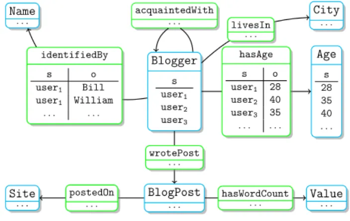
RDF analytical schemas and queries. RDF analytical schemas can be seen as lenses through which data is analyzed. An AnS is a labeled directed graph, whose nodes are analysis classes and whose edges are analysis properties, deemed interesting by the data analyst for a specific analysis task. The instance of an AnS is built from the base data; it is an RDF graph itself, heterogeneous and semantic-rich, restructured for the needs of the analysis.

Figure 1 shows a sample AnS for analyzing bloggers and blog posts. An AnS node is defined by an unary query, which, evaluated over an RDF graph, returns a set of URIs. For instance, the node Blogger is defined by a query which (in this example) returns the URIs user1, user2and

user3. The interpretation is that the AnS defines the analysis class Blogger, whose instances

are these three users. An AnS edge is defined by a binary query, returning pairs of URIs from the base data. The interpretation is that for each (s, o) URI pair returned by the query defining the analysis property p, the triple s p o holds, i.e., o is a value of the property p of s. Crucial for the ability of AnSs to support analysis of heterogeneous RDF graphs is the fact that AnS nodes and edges are defined by completely independent queries. Thus, for instance, a user may be part of the Blogger instance whether or not the RDF graph comprises value(s) for the analysis properties identifiedBy, livesIn etc. of that user. Further, just like in a regular RDF graph, each blogger may have multiple values for a given analysis property. For instance, user1 is

identified both as William and as Bill.

We consider the conjunctive subset of SPARQL consisting of basic graph pattern (BGP) queries, denoted q(¯x):- t1, . . . , tα, where {t1, . . . , tα} are triple patterns. Unless we explicitly

specify that a query has bag semantics, the default semantics we consider is that of set.

The head of q, denoted head(q) is q(¯x), while the body t1, . . . , tα is denoted body(q). We use

Blogger s user1 user2 user3 acquaintedWith . . . Name . . . identifiedBy s o user1 Bill user1 William . . . . City . . . livesIn . . . BlogPost . . . wrotePost . . . Site . . . postedOn . . . hasWordCount. . . Value. . . Age s 28 35 40 . . . hasAge s o user1 28 user2 40 user3 35 . . . .

Figure 1: Sample Analytical Schema (AnS).

where each variable is reachable through triples from a distinguished variable, denoted root. For instance, the following query is a rooted BGP, whose root is x1:

q(x1, x2, x3):- x1 acquaintedWith x2,

x1 identifiedBy y1,

x1 wrotePost y2, y2 postedOn x3

The query’s graph representation below shows that every node is reachable from the root x1.

x1 x2 y1 y2 x3 acquaintedWith identifiedBy wrotePost postedOn

An analytical query consists of two BGP queries homomorphic to the AnS and rooted in the same AnS node, and an aggregation function. The first query, called a classifier, specifies the facts and the aggregation dimensions, while the second query, called the measure, returns the values that will be aggregated for each fact. The measure query has bag semantics. Example 1 presents an AnQ over the AnS defined in Figure 1.

Example 1. Analytical Query The query below asks for the number of sites where each blogger posts, classified by the blogger’s age and city:

Q:- hc(x, dage, dcity), m(x, vsite), counti

where the classifier and measure queries are defined by: c(x, dage, dcity):- x rdf:type Blogger,

x hasAge dage, x livesIn dcity

m(x, vsite):- x rdf:type Blogger,

x wrotePost p, p postedOn vsite

The semantics of an analytical query is:

Definition 2.1. Answer Set of an Analytical Query. Let I be the instance of an analytical schema with respect to some RDF graph. Let Q:- hc(x, d1, . . . , dn), m(x, v), ⊕i be an analytical

query against I.

ans(Q, I) = {hdj₁, . . . , dj

n, ⊕(qj(I))i |

hxj_{, d}j 1, . . . , d

j

ni ∈ c(I)and qj(I)is the bag

of all values vj

k such that (x

j_{, v}j

k) ∈ m(I)}

where qj_{(I) is a bag containing all measure values v corresponding to x}j_{, and the operator ⊕}

aggregates all members of this bag. It is assumed that each value returned by qj_{(I)is of (or can}

be converted by the SPARQL rules [3] to) the input type of the aggregator ⊕. Otherwise, the answer set is undefined. Further, if qj_{(I) is empty, the aggregated measure is undefined, and}

xj does not contribute to the cube. In the following, we only consider analytical queries whose

answer set is defined. Also, for conciseness, we use ans(Q) to denote ans(Q, I), where I is considered the working instance of the analytical schema.

In other words, the AnQ returns each tuple of dimension values from the answer of the classifier query, together with the aggregated result of the measure query for those dimension values. The answer set of an AnQ can thus be represented as a cube of n dimensions, holding in each cube cell the corresponding aggregate measure.

The counterpart of a fact, in this framework, is any value to which the first variable in the classifier, x above, is bound, and that has a non-empty answer for the measure query. In RDF, a resource may have zero, one or several values for a given property. Accordingly, in our framework, a fact may have multiple values for each measure; in particular, some of these values may be identical, yet they should not be collapsed into one. For instance, if a product is rated by 5 users, one of which rate it ? ? ? while the four others rate it ?, the number of times each value was recorded is important. This is why we assign bag semantics to qj_{(I). In all other contexts}

where BGP queries are mentioned in this work, they have set semantics; this holds in particular for any classifier query c(x, d1, . . . , dn).

Example 2. Analytical Query Answer Consider the AnQ in Example 1, over the AnS in Fig-ure 1. Suppose the classifier query’s answer set is:

{huser1, 28, Madridi, huser3, 35, NYi, huser4, 35, NYi}

the measure query is evaluated for each of the three facts, leading to the intermediary results: xj

user1 user3 user4

qj_{(I) {|hs}

1i, hs1i, hs2i|} {|hs2i|} {|hs3i|}

where {|·|} denotes the bag constructor. Aggregating the sites among the classification dimensions leads to the AnQ answer:

{h28, Madrid, 3i, h35, NY, 2i}

OLAP for RDF.On-Line Analytical Processing (OLAP) [4] technologies enhance the abilities of data warehouses (so far, mostly relational) to answer multi-dimensional analytical queries. In a relational setting, the so-called “OLAP operations” allow computing a cube (the answer to an analytical query) out of another previously materialized cube.

In our data warehouse framework specifically designed for graph-structured, heterogeneous RDF data, a cube corresponds to an AnQ; for instance, the query in Example 1 models a bi-dimensional cube on the warehouse related to our sample AnS in Figure 1. Thus, we model traditional OLAP operations on cubes as AnQ rewritings, or more specifically, rewritings of extended AnQs which we introduce below.

Definition 2.2. Extended AnQ. Let S be an AnS, and d1, . . . , dn be a set of dimensions, each ranging over a non-empty finite set Vi. Let Σ be a

total function over {d1, . . . , dn}associating to each di, either Vi or a non-empty subset of Vi. An

extended analytical query Q is defined by a triple:

Q:- hcΣ(x, d1, . . . , dn), m(x, v), ⊕i

where c is a classifier and m a measure query over S, ⊕ is an aggregation operator, and moreover: cΣ(x, d1, . . . , dn) =S(χ1,...,χn)∈Σ(d1) × ...×Σ(dn)c(x, χ1, . . . , χn)

In the above, the extended classifier cΣ(x, d1, . . . , dn)is the set of all possible classifiers

ob-tained by replacing each dimension variable di with a value from Σ(di). We introduce Σ to

constrain some classifier dimensions, i.e., to restrict the classifier result. The semantics of an extended analytical query is derived from the semantics of a standard AnQ (Definition 2.1) by replacing the tuples from c(I) with tuples from cΣ(I). Thus, an extended analytical query can be

seen as a union of a set of standard AnQs, one for each combination of values in Σ(d1), . . . , Σ(dn).

Conversely, an analytical query corresponds to an extended analytical query where Σ only con-tains pairs of the form (di, Vi).

We define the following RDF OLAP operations:

A slice operation binds an aggregation dimension to a single value. Given an extended query Q:- hcΣ(x, d1, . . . , dn), m(x, v), ⊕i, a slice operation over a dimension di with value vi returns

the extended query Qslice:- hcΣ0(x, d1, . . . , dn), m(x, v), ⊕i, where Σ

0 _{= (Σ \ {(d}

i, Σ(di))}) ∪

{(di, {vi})}.

Similarly, a dice operation constrains several aggregation dimensions to values from specific sets. A dice on Q over dimensions {di1, . . . , dik}and corresponding sets of values {Si1, . . . , Sik},

returns the query Qdice:- hcΣ0(x, d₁, . . . , d_n), m(x, v), ⊕i, where Σ0= (Σ \Si_j=ik

1{(dj, Σ(dj))}) ∪

Sik

j=i1{(dj, Sj)}.

A drill-out operation on Q over dimensions {di1, . . . , dik}corresponds to removing these

di-mensions from the classifier. It leads to a new query Qdrill-outhaving the classifier cΣ0(x, d_j 1, . . . ,

djn−k), where dj1, . . . , djn−k ∈ {d1, . . . , dn} \ {di1, . . . , dik} and Σ

0_{= (Σ \}Sik

j=i1{(dj, Σ(dj))}).

Finally, a drill-in operation on Q over dimensions {dn+1, . . . , dn+k} which all appear in the classifier’s body and have value sets {Vn+1, . . . , Vn+k}

corresponds to adding these dimensions to the head of the classifier. It produces a new query

Q_drill-inhaving the classifier cΣ0(x, d₁, . . . , d_n, d_n+1, . . . , d_n+k), where the dimensions d_n+1, . . . , d_n+k

6∈ {d1, . . . , dn}, and Σ0 = (Σ ∪S

ik

j=i1{(dj, Vj)}).

These operations are illustrated in the following example.

Example 3. OLAP Operations. Let Q be the extended query corresponding to the query-cube defined in Example 1, that is: Q:- hc(x, age, city), m(x, site), counti Σ = {(age, Vage),

(city, Vcity)} (the classifier and measure are as in Example 1).

A slice operation on the age dimension with value 35 replaces the extended classifier of Q with cΣ0(x, age, city) = {c(x, 35, city)} where Σ0 = Σ \ {(age, V_age)} ∪ {(age, {35})}.

A dice operation on both age and city dimensions with values {28} for age and {Madrid, Kyoto} for city replaces the extended classifier of Q with cΣ0(x, age, city) = {c(x, 28, Madrid), c(x, 28, Kyoto)}

where Σ0_{= {(age, {28}), (city, {Madrid, Kyoto})}.}

A drill-out on the age dimension produces Qdrill-out

:-hc0

Σ0(x, city), m(x, site), counti with Σ0 = {(city, Vcity)} and body(c0) ≡ body(c).

Finally, a drill-in on the age dimension applied to the query Qdrill-out above produces Q,

Analytical query Q

Analytical query QT

apply OLAP transf. T (described in Section 2)

Answer to Q – ans(Q) d1 d2 . . . dn v

Intermediary result – pres(Q) x d1 d2 . . . dn k m evaluate c and m of Q on I aggregate column m Answer to QT d1 d2 . . . dm v evaluate QT on I

How to simulate the transf. T by rewriting QT using pres(Q)

or ans(Q) (and I if necessary).

Figure 2: Problem statement.

3

Optimized OLAP operations

The above OLAP operations lead to new queries, whose answers can be computed based on the AnS instance. The focus of the present work is on answering such queries by using the materialized results of the initial AnQ, and (only when that input is insufficient) more data, such as intermediary results generated while computing AnQ results, or (a small part of) the AnSinstance. These results are often significantly smaller than the full instance, hence obtaining the answer to the new query based on them is likely faster than computing it from the instance. Figure 2 provides a sketch of the problem.

In the following, all relational algebra operators are assumed to have bag semantics.

Given an analytical query Q whose measure query (with bag semantics) is m, we denote by ¯

m the set-semantics query whose body is the same as the one of m and whose head comprises all the variables of m’s body. Obviously, there is a bijection between the bag result of m and the set result of ¯m. Using ¯m, we define next the intermediary answer of an AnQ.

Definition 3.1. Intermediary query of an AnQ. Let Q:- hc, m, ⊕i be an AnQ. The intermediary query of Q, denoted int(Q), is:

int(Q) = c(x, d1, . . . , dn) ./xm(x, v)¯

It is easy to see that int(Q) holds all the information needed in order to compute both c and m; it holds more information than the results of c and m, given that it preserves all the different embeddings of the (bag-semantics) m query in the data. Clearly, evaluating int is at least as expensive as evaluating Q itself; while int is conceptually useful, we do not need to evaluate it or store its results.

Instead, we propose to evaluate (possibly as part of the effort for evaluating Q), store and reuse a more compact result, defined as follows. For a given query Q whose measure (with bag semantics) is m, we term extended measure result over an instance I, denoted mk_{(I), the set}

{(newk(), t) | t ∈ m(I)}

where newk() is a key-creating function returning a distinct value at each call. A very simple implementation of newk(), which we will use for illustration, returns successively 1, 2, 3 etc. We assign a key to each tuple in the measure so that multiple identical values of a given measure for a given fact would not be erroneously collapsed into one. For instance, if

m(I) = {|(x1, m1), (x1, m1), (x1, m2), (x2, m3)|}

then:

mk_{(I) = {(1, x}

1, m1), (2, x1, m1), (3, x1, m2), (4, x2, m3)}

Definition 3.2. Partial result of an AnQ. Let Q:- hc, m, ⊕i be an AnQ. The partial result of Qon an instance I, denoted pres(Q, I) is:

pres(Q, I) = c(I) ./xmk(I)

One can see pres(Q, I) as the input to the last aggregation performed in order to answer the AnQ, augmented with a key. In the following, we use pres(Q) to denote pres(Q, I) for the working instance of the AnS.

Problem Statement 1. (Answering AnQs using the materialized results of other AnQ.) Let Q,QT be AnQs such that applying the OLAP transformation T on Q leads to QT.

The problem of answering AnQ using the materialized result of AnQ consists of finding: (i) an equivalent rewriting of QT based on pres(Q) or ans(Q), if one exists; (ii) an equivalent rewriting

of QT based on pres(Q) and the AnS instance, otherwise.

Importantly, the following holds:

πx,d1,...,dn,v(int(Q)(I)) = πx,d1,...,dn,v(pres(Q, I)) (1)

Q ≡ γd1,...,dn,⊕(v)(πx,d1,...,dn,v(int(Q))) (2)

ans(Q)(I) = γd1,...,dn,⊕(v)(πx,d1,...,dn,v(pres(Q, I))) (3)

Equation (1) directly follows from the definition of pres. Equation (2) will be exploited to establish the correctness of some of our techniques. Equation (3) above is the one on which our rewriting-based AnQ answering technique is based.

3.1

Slice and Dice

In the case of slice and dice operations, the data cube transformation is made simply by row selection over the materialized final results of an AnQ.

Example 4. Dice. The query Q asks for the average number of words in blog posts, for each blogger’s age and residential city.

Q:- hc(x, age, city), m(x, words), averagei c(x, age, city):- x rdf:type Blogger, x hasAge age, x livesIn city

m(x, site):- x rdf:type Blogger, x wrotePost p, p hasWordCount words Suppose the answer of c over I is

and the answer of m over I is

{|huser1, 100i, huser1, 120i, huser3, 570i, huser4, 410i|}

Joining the answers of c and m in such a query results in:

{|huser1, 28, Madrid, 100i, huser1, 28, Madrid, 120i,

huser3, 35, NY, 570i, huser4, 28, Madrid, 410i|}

The final answer to Q after aggregation is:

{h28, Madrid, 210i, h35, NY, 570i}

The query Qdice is the result of a dice operation on Q, restricting the age to values between

20 and 30. Q_dice differs from Q only by its classifier which can be written as cΣ0(x, age, city)

where Σ0_{= Σ \ {(age, {age})} ∪ {(age, {age}}

20≤age≤30)}.

Applying dice on the answer to Q above yields the result: {h28, Madrid, 210i}

Now, we calculate the answer to Qdice. The result of the classifier query cΣ0, obtained by applying

a selection on the age dimension is:

{huser1, 28, Madridi, huser4, 28, Madridi}

Evaluating m and joining its result with the above set yields:

{|huser1, 28, Madrid, 100i, huser1, 28, Madrid, 120i,

huser4, 28, Madrid, 410i|}

The final answer to Qdice after aggregation is:

{h28, Madrid, 210i} dice applied over the answer of Q yields the answer of Qdice.

Definition 3.3. Selection. Let dice be a dice operation on analytical queries. Let Σ0 be the function introduced in Definition 2.2. We define a selection σdice as a function on the space of

analytical query answers ans(Q) where:

σdice(ans(Q)) = {hd1, . . . , dn, vi|hd1, . . . , dn, vi ∈ ans(Q)

∧ ∀i ∈ {1, . . . , n} di∈ Σ0(di)}

Proposition 3.1. Let Q:- hc(x, d1, . . . , dn), m(x, v), ⊕iand Qdice:- hcΣ0(x, d₁, . . . , d_n), m(x, v), ⊕i

be two analytical queries such that query Qdice= dice(Q). Then: σdice(ans(Q)) = ans(Qdice).

Proof. The proof follows from two-way inclusion; σdice(ans(Q)) ⊆ ans(Qdice)and σans(Q_dice)⊆

dice(ans(Q)).

We first show that each tuple in σdice(ans(Q)) is also a member of ans(Q_dice). Let t =

(a1, . . . , an, V ) ∈ ans(Q) (4)

∀i ∈ {1, . . . , n} ai∈ Σ0(di) (5)

Since t ∈ σdice(ans(Q)), there is a set of tuples of the form (x, a1, . . . , an)in c(I); we denote

this set by Ac. From (5) it follows that Ac⊆ cΣ0(I), therefore A_conxmk(I) ⊆ c_Σ0(I) o_nxmk(I)

and there is a tuple such as (a1, . . . , an, W )in ans(Qdice). We call this tuple u.

Furthermore, let Ac_Σ0 be the set of all tuples of the form (x, a1, . . . , an) in cΣ0(I). Since

cΣ0(I) ⊆ c(I), we have A_c

Σ0 ⊆ c(I). From the definition of Ac, it follows that AcΣ0 = Ac and:

Ac_Σ0 onxmk(I) = Ac onxmk(I)(*)

V is the result of aggregation over the measure values in Aconxmk(I)and W is the result of

aggregation over the measure values in Ac_Σ0 onxmk(I). Therefore based on (*), V = W , t = u,

hence t ∈ ans(Qdice). This concludes the first part of the proof.

We will now show that each tuple in ans(Qdice) is also a member of σdice(ans(Q)). Let

(a0₁, . . . , a0_n, V0)be a tuple in in ans(Q_dice), by definition we have: ∀i ∈ {1, . . . , n}, a0i∈ Σ0(di)

It remains to prove that (a0

1, . . . , a0n, V0) ∈ ans(Q). First, if (a10, . . . , a0n, V0) ∈ ans(Qdice),

then there is a set of tuples of the form (x, a0

1, . . . , a0n)in c0(I). By definition of dice, we have

c0(I) ⊆ c(I), therefore c0_{(I) on}x mk(I) ⊆ c(I) onx mk(I) and hence, a tuple t0 with dimension

values a0

1, . . . , a0n exists in ans(Q). Second, we can use an argument similar to the previous part

of the proof to show that t0 _{has the same aggregated measure value as V}0_{. This concludes the}

second part of the proof.

3.2

Drill-Out

Unlike the relational DW setting, in our RDF warehousing framework the result of a drill-out operation (that is, the answer to Qdrill-out) cannot be correctly computed directly from the

answer to the original query Q, and here is why. Each tuple in ans(Q) binds a set of dimension values to an aggregated measure. In fact, each such tuple represents a set of facts having the same dimension values. Projecting a dimension out will make some of these sets merge into one another, requiring a new aggregation of the measure values. Computing this new aggregated measure from the ones in ans(Q) will require considering whether the aggregation function has the distributive property, i.e., whether ⊕(a, ⊕(b, c)) = ⊕(⊕(a, b), c).

1. Distributive aggregation function, e.g. sum. In this case, the new aggregated measure value could be computed from ans(Q) if the sets of facts aggregated in each tuple of ans(Q) were mutually exclusive. This is not the case in our setting where each fact can have several values along the same dimension. Thus, aggregating the already aggregated measure values will lead to erroneously consider some facts more than once; avoiding this requires being able to trace the measure results back to the facts they correspond to.

2. Non-distributive aggregation function, e.g., avg. For such functions, the new aggregated measure must be computed from scratch.

Based on the above discussion, we propose Algorithm 1 to compute the answer to Qdrill-out,

using the partial result of Q, denoted pres(Q) above, which we assume has been materialized and stored as part of the evaluation of the original query Q. This deduplication (δ) step is needed, since some facts may have been repeated in T for being multivalued along di. The aggregation

Algorithm 1: drill-out cube transformation

1: Input: pres(Q), di

2: T ← Πroot,d1,...,di−1,di+1,...,dn,k,v(pres(Q))

3: T ← δ(T )

4: T ← γd1,...,di−1,di+1,...,dn,⊕(v)(T )

5: return T

function ⊕ is applied to the measure column of the resulting relation T , using γ, grouping the tuples along the dimensions dProposition 3.2 states the correctness of Algorithm 1.1, . . . , di−1, di+1, . . . , dn.

Proposition 3.2. Let Q be an AnQ and Q_drill-out be the AnQ obtained from Q by drilling out along the dimension di. Algorithm 1 applied on pres(Q) and di computes ans(Q_drill-out).

Example 5 illustrates Algorithm 1, and also shows how relying only on ans(Q) may introduce errors.

Example 5. Drill-out. Consider an analytical query Q such that its classifier c1, measure m

and intermediary answer pres(Q) have the results shown below. c1 root d1 . . . dn−1 dn x a1 . . . an−1 an x a1 . . . an−1 bn y a1 . . . an−1 bn m k root v 1 x m1 2 y m2 pres(Q) root d1 . . . dn−1 dn k v x a1 . . . an−1 an 1 m1 x a1 . . . an−1 bn 1 m1 y a1 . . . an−1 bn 2 m2 (i)

Let Qdrill-out be the result of a drill-out operation on Q eliminating dimension dn. The

measure of Qdrill-out is still m, while its classifier c2 has the answer shown next:

c2

root d1 . . . dn−1

x a1 . . . an−1

y a1 . . . an−1

Note that c2 returns only one row for x, because it has one value for the dimension vector

hd1, . . . , dn−1i. pres(Qdrill-out)yields:

root d1 . . . dn−1 k v

x a1 . . . an−1 1 m1

y a1 . . . an−1 2 m2

d1 . . . dn−1 v

a1 . . . an−1 ⊕({m1, m2})

(ii)

Algorithm 1 on the input (i), first projects out dn. Table T after projecting out dn from

pres(Q)is:

root d1 . . . dn−1 k v

x a1 . . . an−1 1 m1

x a1 . . . an−1 1 m1

y a1 . . . an−1 2 m2

The duplicate tuples are eliminated (δ(T )), resulting in: root d1 . . . dn−1 k v

x a1 . . . an−1 1 m1

y a1 . . . an−1 2 m2

Finally we apply grouping and aggregation on the above table: d1 . . . dn−1 v

a1 . . . an−1 ⊕({m1, m2})

(iii)

The output of Algorithm 1 above, denoted (iii), is the same as (ii), showing that our algorithm answers Qdrill-out correctly using the intermediary answer of Q.

Next we examine what would happen if an algorithm took the answer of Q as input. First, we compute ans(Q), by aggregating the measures along the dimensions from the intermediary result depicted in (i):

ans(Q)

d1 . . . dn−1 dn v

a1 . . . an−1 an ⊕({m1})

a1 . . . an−1 bn ⊕({m1, m2})

Next we project out dn from ans(Q):

d1 . . . dn−1 v

a1 . . . an−1 ⊕({m1})

a1 . . . an−1 ⊕({m1, m2})

and aggregate, assuming that ⊕ is distributive. d1 . . . dn−1 v

a1 . . . an−1 ⊕({m1, m1, m2})

(iv)

Observe that (iv) is different from (ii). More specifically, the measure value corresponding to the multi-valued entity x has been considered twice in the aggregated measure value of (iv).

3.3

Drill-In

The drill-in operation increases the level of detail in a cube by adding a new dimension. In general, this additional information is not present in the answer of the original query. Hence, answering the new query requires extra information.

Algorithm 2: drill-in cube transformation

1: Input: pres(Q, I), c, dn+1

2: build qQ

aux(dvars, dn+1):- body (as per Definition 3.4)

3: T ← pres(Q, I) ondvarsans(qQaux)(I)

4: T ← γd1,...,dn,dn+1,⊕(v)(T )

5: return T

Algorithm 2 uses the partial result of Q, denoted pres(Q), and consults the materialized AnS instance to obtain the missing information necessary to answer Q_drill-in. We retrieve this information through an auxiliary query defined as follows.

Definition 3.4. Auxiliary drill-in query. Let Q:- hc(x, d1, . . . , dn), m(x, v), ⊕i be an AnQ

and dn+1 a non-distinguished variable in c. The auxiliary drill-in query of Q over dn+1 is a

conjunctive query qQ

aux(dvars, dn+1):- bodyaux, where

• each triple t ∈ body(c) containing the variable dn+1 is also in bodyaux;

• for each triple taux in bodyaux and t in the body of c such that t and taux share a

non-distinguished variable of c, the triple t also belongs to bodyaux;

• each variable in bodyaux that is distinguished in c is a distinguished variable qauxQ .

The auxiliary query qQ

aux comprises all triples from Q’s classifier having the dimension dn+1;

to these, it adds all the classifier triples sharing a non-distinguished (existential) variable with the former; then all the classifier triples sharing an existential variable with a triple previously added to bodyaux etc. This process stops when there are no more existential variables to consider. The

variables distinguished in c, together with the new dimension dn+1, are distinguished in qQaux.

Proposition 3.3. Let Q:- hc, m, ⊕i be an analytical query and dn+1 be a non-distinguished

variable in c. Let Qdrill-in be the analytical query obtained from Q by drilling in along the

dimension dn+1, and I be an instance. Algorithm 2 applied on pres(Q, I), c, and dn+1computes

ans(Q_drill-in)(I).

Proof. The correctness of Algorithm 2 boils down to showing that joining pres(Q, I), with qQ

aux(I), and aggregating the measure values v along the dimensions d1, . . . , dn+1 produces the

answer to Qdrill-in.

We must therefore prove that:

γd1,...,dn,dn+1,⊕(v)(int(Qdrill-in))(I) =

γd1,...,dn,dn+1,⊕(v)(πx,...,dn+1(pres(Q, I) ondvarsq

Q aux(I)))

Or, as stated in Section 3:

γd1,...,dn,dn+1,⊕(v)(πx,...,dn+1(pres(Q, I))) =

γd1,...,dn,dn+1,⊕(v)(πx,...,dn+1(int(Q))(I))

γd1,...,dn,dn+1,⊕(v)(int(Qdrill-in))(I) =

γd1,...,dn,dn+1,⊕(v)(πx,...,dn+1(int(Q) ondvarsq

Q aux)(I))

Since the aggregation is the same, it suffices to show that: int(Q_{drill-in) = int(Q) on}dvarsqauxQ

We show that the join expression above is an equivalent rewriting of int(Qdrill-in), in other

words that:

c_drill-in./xm¯drill-in≡ c ./xm ./¯ dvarsqQaux

or equivalently (since Q and Qdrill-in have the same measure):

c_drill-in./xm ≡ c ./¯ xm ./¯ dvarsqauxQ

It is easy to see that the queries on one side and the other of the ≡ sign have the same head vari-ables, namely x, d1, d2, . . . , dn+1. Further, given that the classifier and measure are independent

queries, the above holds if and only if:

c_drill-in≡ c ./dvarsqQaux

To establish the above, we note that an obvious homomorphism exists from the body of

c_drill-in into the union of the atoms in c’s body and those in the body of qQ

aux, given that the

body of cdrill-inis exactly that of c. Conversely, by construction, the atoms in the body of qQaux

are a subset of those in the body of c (thus, cdrill-in), thus an obvious homomorphism holds

from c ./vars qQaux. Further, both homomorphisms map the free variables if int(Qdrill-in) to

themselves, concluding the equivalence proof.

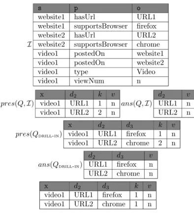
Example 6. Drill-in rewriting. Let Q:- hc, m, sumi be the query counting videos, classified by the URL of the website on which they are uploaded.

c(x, d2):- x rdf:type Video, x uploadedOn d1,

d1 hasUrl d2, d1 supportsBrowser d3

m(x, v):- x rdf:type Video, x viewNum v

Q_drill-in is the result of a drill-in that adds the dimension d3, having the classifier query

c0(x, d2, d3).

Figure 3 shows the materialized analytical schema instance, the partial and final answer to Q, and the partial and final answer to Qdrill-in. Now, let us see how to answer Qdrill-in using

Algorithm 2. We have: qQ

aux(x, d2, d3):- x postedOn d1, d1 hasUrl d2,

d1 supportsBrowser d3

Based on I, the answer to qQ

aux is:

x d2 d3

video1 URL1 firefox video1 URL2 chrome

I

s p o

website1 hasUrl URL1 website1 supportsBrowser firefox website2 hasUrl URL2 website2 supportsBrowser chrome video1 postedOn website1 video1 postedOn website2 video1 type Video video1 viewNum n pres(Q, I) x d2 k v video1 URL1 1 n video1 URL2 2 n ans(Q, I) d2 v URL1 n URL2 n pres(Q_drill-in) x d2 d3 k v

video1 URL1 firefox 1 n video1 URL2 chrome 2 n ans(Q_drill-in)

d2 d3 v

URL1 firefox n URL2 chrome n x d2 d3 k v

video1 URL1 firefox 1 n video1 URL2 chrome 1 n

Figure 3: drill-in example.

Joining the above with pres(Q) yields the last table in Figure 3, which after aggregation yields the result of Qdrill-in.

4

Experiments

We demonstrate the performance of our RDF analytical framework through a set of experiments. Section 4.1 outlines our implementation and experimental settings, while Section 4.2 presents experimental results, then we conclude.

4.1

Implementation and settings

We deployed our analytics framework on top of a PostgreSQL relational server version 9.3.2 and evaluate all queries by translating them into SQL.

Data organization. The AnQs are evaluated against the instance I stored into a dictionary encoded triples table indexed by all permutations of the s, p, o columns.

Dataset. We test our algorithms using the LUBM generated dataset of about 1 million triples, and a simple AnS having a node for every class in the dataset and an edge for every property; this amounts to an analytical schema whose description consists of 234 triples.

Queries. We test our algorithms using a set of six AnQs. These queries have between 40320 and 426 triples (average 11652) and each have either three or four classification dimensions (average 3.5). The full queries are shown below.

1. count advisor students: the number of students that heads of department advise, classified by the department which they are head of, the university the department is in, and the university they have gotten their degree from.

QAdvStu:- hcAdvStu(pr, dp, udp, udg), mAdvStu(pr, st), counti

cAdvStu(pr, dp, udp, udg)

:-pr rdf:type lubm:Professor, :-pr lubm:headOf dp, dp rdf:type lubm:Department, dp lubm:subOrganizationOf udp, udp rdf:type lubm:University,

pr lubm:degreeFrom udg, udg rdf:type lubm:University

mAdvStu(pr, st)

:-pr rdf:type lubm:Professor, st lubm:advisor :-pr, st rdf:type lubm:Student

2. count lecturer courses: the number of courses lecturers teach, classified by the department which they are a member of, the university the department is in and the university from which they have a degree.

QLctCou:- hcLctCou(lc, dp, udp, udg), mLctCou(lc, co), counti

cLctCou(lc, dp, udp, udg)

:-lc rdf:type lubm:Lecturer, :-lc lubm:memberOf dp,

dp rdf:type lubm:Department, dp lubm:subOrganizationOf udp,

udp rdf:type lubm:University, lc lubm:teacherOf co, co rdf:type lubm:Course, lc lubm:degreeFrom udg, udg rdf:type lubm:University

mLctCou(lc, co)

:-lc rdf:type lubm:Lecturer, :-lc lubm:teacherOf co, co rdf:type lubm:Course

3. count lecturer departments: the number of departments lecturers are members of, classified by the university the department is in, the courses they teach, and the university from which they have a degree.

QLctDep:- hcLctDep(lc, udp, co, udg), mLctDep(lc, dp), counti

cLctDep(lc, udp, co, udg)

:-lc rdf:type lubm:Lecturer, :-lc lubm:memberOf dp, dp rdf:type lubm:Department, dp lubm:subOrganizationOf udp, udp rdf:type lubm:University,

lc lubm:teacherOf co, co rdf:type lubm:Course, lc lubm:degreeFrom udg, udg rdf:type lubm:University

mLctDep(lc, dp)

:-lc rdf:type lubm:Lecturer, :-lc lubm:memberOf dp, dp rdf:type lubm:Department 4. count professor graduate courses: the number of graduate courses professors teach,

classi-fied by the professor’s department, the university for which she works, the university from which she got her degree, and the course she teaches.

QP rf Grd:- hcP rf Grd(pr, dp, upr, udg, co), mP rf Grd(pr, gco), counti

cP rf Grd(pr, dp, upr, udg, co)

:-pr rdf:type lubm:Professor, :-pr lubm:worksFor dp, dp rdf:type lubm:Department, dp lubm:subOrganizationOf upr, upr rdf:type lubm:University,

pr lubm:degreeFrom udg, udg rdf:type lubm:University, pr lubm:teacherOf co, co rdf:type lubm:Course

mP rf Grd(pr, gco)

:-pr rdf:type lubm:Professor, :-pr lubm:teacherOf gco, gco rdf:type lubm:GraduateCourse

classified by the department they work for, the university of that department, the university from which they have gotten their degree and their advisor.

QResCou:- hcResCou(ra, dp, udp, udg, ad), mResCou(ra, co), counti

cResCou(ra, dp, udp, udg, ad)

:-ra rdf:type lubm:ResearchAssistant, :-ra lubm:memberOf dp, dp rdf:type lubm:Department, dp lubm:subOrganizationOf udp, udp rdf:type lubm:University, ra lubm:degreeFrom udg,

udg rdf:type lubm:University, ra lubm:advisor ad, ad rdf:type lubm:Professor

mResCou(ra, co)

:-ra rdf:type lubm:ResearchAssistant, :-ra lubm:takesCourse co, co rdf:type lubm:Course

6. count student courses: the number of courses students have taken, classified by the student’s department, university, advisor and the university where the advisor has obtained a degree.

QStuCou:- hcStuCou(st, dp, ust, ad, uad), mStuCou(st, co), counti

cStuCou(st, dp, ust, ad, uad)

:-st rdf:type lubm:Student, :-st lubm:memberOf dp, dp rdf:type lubm:Department, dp lubm:subOrganizationOf ust, ust rdf:type lubm:University,

st lubm:advisor ad, ad rdf:type lubm:Professor,

ad lubm:degreeFrom uad, uad rdf:type lubm:University

mStuCou(st, co)

:-st rdf:type lubm:Student, :-st lubm:takesCourse co, co rdf:type lubm:Course

Hardware. The experiments ran on an 8-core DELL server at 2.13 GHz with 16 GB of RAM, running Linux 2.6.31.14. All times we report are averaged over five executions.

4.2

Experiment results

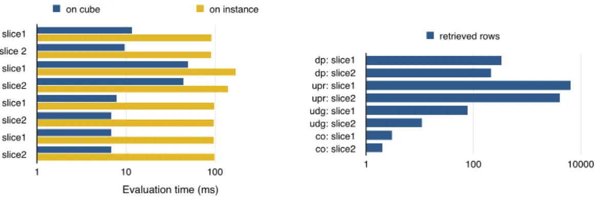
Slice and Dice. Figure 4 shows the evaluation time of Q_slice on the materialized instance vs. its evaluation time on the materialized cube, i.e. the final result of Q. This time is shown for one arbitrary dimension in each query. Two slice experiments are conducted for each dimension: one by the most frequent value of the dimension in the cube, and one by the least frequent one. The figure clearly shows that evaluating the queries on the cube using our algorithm is much more efficient than their evaluation on the analytical instance.

Figure 5 shows the evaluation time and number of retrieved rows of slice on all of the dimen-sions of query QP rf Grd, each with two value. Note the correlation between the query evaluation

time and the query result size.

Figure 6 shows the evaluation time of Qdiceon the analytical instance vs. its evaluation time

on the cube. In each dice experiment, selections on two dimensions of each query are made. The values picked for selections are manually chosen, in a way that the number of retrieved rows are diverse enough, and the result of dice is non-empty.

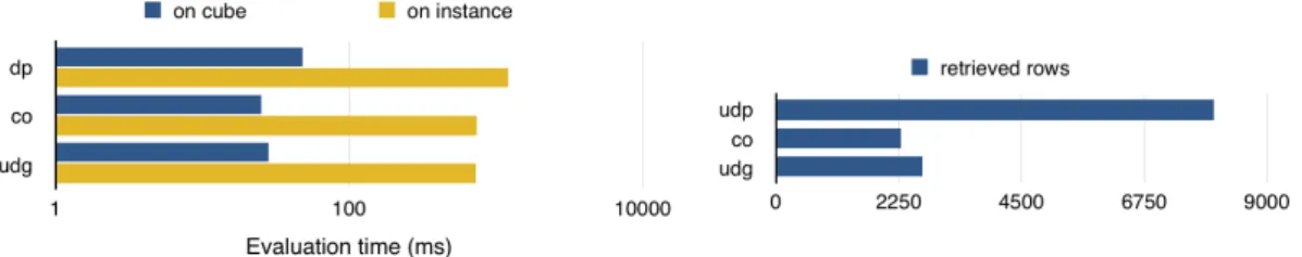
Drill-out. Figure 7 shows the time of evaluating Q_drill-out on the cube vs. the time of its evaluation on the analytical instance. The figure shows the evaluation times for one dimension per query. As we see, the queries are evaluated much faster on the cube using our algorithm. Figure 8 shows the evaluation time and number of retrieved rows of Qdrill-outfor three different

dimensions of the same query. The figure shows that for a specific size of cube, the evaluation time of Qdrill-out is correlated with the number of tuples that it retrieves.

Figure 4: Evaluation time for slice on all queries.

Figure 5: Evaluation time and number of rows retrieved for slice on query QP rf Grd(four dimensions).

Figure 6: Evaluation time for dice on all queries.

on the analytical instance for five different queries. The queries used for drill-in experiments have the same body as the ones used in previous experiments in this paper, except that they only have one dimension in their head before drill-in is applied.

As Figure 9 shows, in most cases, the evaluation time of Qdrill-in on the cube is more than

its evaluation time on the analytical instance. This is because qQ

aux retrieves more tuples than

the classifier of Q, qQ

Figure 7: Evaluation time for drill-out on all queries.

Figure 8: Evaluation time and number of retrieved rows for different drill-out operations on QLctDep (three dimensions).

Figure 9: Evaluation time for drill-in on all queries.

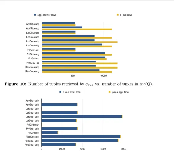
the result of qaux in comparison to the number of tuples in the intermediary answer of the query.

As seen in the figure, the size of qaux’s answer is huge in comparison to the intermediary answer

(notice the logarithmic scale). As a consequence, the cost of retrieving and joining the increased number of tuples is quite significant. Figure 11 breaks down the view-based evaluation of the drilled-in query in two: the time to evaluate qaux, and the time to evaluate the join between qaux

and pres(Q), the latter being stored as an non-indexed temporary table in the database. As we see, the bulk of the evaluation time is used on evaluating qaux on the instance. The effect of the

time of evaluating join is merely marginal.

These observations point to the fact that our view-based evaluation strategies for drilled-in queries is currently not competitive with re-evaluation from scratch. We will continue work to investigate more efficient strategies for this task, as part of our future work.

Figure 10: Number of tuples retrieved by qauxvs. number of tuples in int(Q).

Figure 11: Time of evaluation of drill-in query on cube: time of evaluation of qauxand time of joining it with int(Q).

5

Related Work

In the area of RDF data management, previous works focused on efficient stores [5, 6, 7], index-ing [8], query processindex-ing [9] and multi-query optimization [10], view selection [11] and query-view composition [12], or Map-Reduce based RDF processing [13, 14]. BGP query answering tech-niques have been studied intensively, e.g., [15, 16], and some are deployed in commercial systems such as Oracle 11g, which provides a “Semantic Graph” extension etc. Given the generality of the RDF analytics framework [1] on which this work is based, the optimizations presented here can be efficiently deployed on top of any RDF data management platform, to extend it with optimized analytic capabilities. Previous RDF data management research focused on efficient stores, query processing, view selection etc. BGP query answering techniques have been studied intensively, e.g., [15, 16], and some are deployed in commercial systems such as Oracle 11g’s “Semantic Graph” extension. Our optimizations can be deployed on top of any RDF data management platform, to extend it with optimized analytic capabilities.

The techniques we presented follow the ideas of query rewriting using views: we use the materialized partial or final AnQ results as a view. View-based query answering has been amply discussed for several contexts [17]. Query optimization is considered the most obvious use of query rewriting. In this work we aims at finding all the answers to the query that exist in the database. The typical difficulties that arise in settings involving grouping and aggregation are the fact that aggregation may partially project out needed attributes and that grouping causes multiplicity loss in attribute values. Apart from these difficulties, our RDF specific framework

has to also deal with heterogeneous data.

SPARQL 1.1 [3] features SQL-style grouping and aggregation, less expressive than our AnQs, as our measure queries allow more flexibility than SPARQL. Thus, the OLAP operation opti-mizations we presented can also apply to the more restricted SPARQL analytical context.

OLAP has been thoroughly studied in a relational setting, where it is at the basis of a successful industry; in particular, OLAP operation evaluation by reusing previous cube results is well-known. The heterogeneity of RDF, which in turn justified our novel RDF analytics framework [1], leads to the need for the novel algorithms we described here, which are specific to this setting.

6

Conclusion

Our work focused on optimizing the OLAP transformations in the RDF data warehousing frame-work we introduced in [1], by using view-based rewriting techniques. To this end, for each OLAP operation, we introduced an algorithm that answers a transformed query based on the final or on an intermediary result of the original analytical query.

The correctness of these algorithms have been shown, for any aggregation function, and the experimental results show that the algorithms for slice, dice and drill-out drastically improve the efficiency of query answering, decreasing query execution time by an order of magnitude. In the case of drill-in however, the cube transformation algorithm is less efficient than query execution on the analytical instance, leaving this case open for future work. Cube transformation algorithms for roll-up and drill-down, and a theoretical discussion on the minimum amount of data that needs to be stored for cube transformation algorithms to work are other open areas for future work.

References

[1] D. Colazzo, F. Goasdoué, I. Manolescu, and A. Roatis, “RDF analytics: lenses over semantic graphs,” in WWW, 2014.

[2] S. Spaccapietra, E. Zimányi, and I. Song, eds., Journal on Data Semantics XIII, vol. 5530 of LNCS, Springer, 2009.

[3] W3C, “SPARQL 1.1 query language.” http://www.w3.org/TR/sparql11-query/, March 2013.

[4] “OLAP council white paper.” http://www.olapcouncil.org/research/resrchly.htm.

[5] D. J. Abadi, A. Marcus, S. R. Madden, and K. Hollenbach, “Scalable semantic web data management using vertical partitioning,” in VLDB, 2007.

[6] M. A. Bornea, J. Dolby, A. Kementsietsidis, K. Srinivas, P. Dantressangle, O. Udrea, and B. Bhattacharjee, “Building an efficient RDF store over a relational database,” in SIGMOD Conference, pp. 121–132, 2013.

[7] L. Sidirourgos, R. Goncalves, M. Kersten, N. Nes, and S. Manegold, “Column-store support for RDF data management: not all swans are white,” PVLDB, vol. 1, no. 2, 2008.

[8] C. Weiss, P. Karras, and A. Bernstein, “Hexastore: sextuple indexing for Semantic Web data management,” PVLDB, vol. 1, no. 1, 2008.

[9] T. Neumann and G. Weikum, “The RDF-3X engine for scalable management of RDF data,” VLDB J., vol. 19, no. 1, 2010.

[10] W. Le, A. Kementsietsidis, S. Duan, and F. Li, “Scalable multi-query optimization for SPARQL,” in ICDE, pp. 666–677, 2012.

[11] F. Goasdoué, K. Karanasos, J. Leblay, and I. Manolescu, “View selection in Semantic Web databases,” PVLDB, vol. 5, no. 1, 2012.

[12] W. Le, S. Duan, A. Kementsietsidis, F. Li, and M. Wang, “Rewriting queries on SPARQL views,” in WWW, pp. 655–664, 2011.

[13] J. Huang, D. J. Abadi, and K. Ren, “Scalable SPARQL Querying of Large RDF Graphs,” PVLDB, vol. 4, no. 11, 2011.

[14] M. Husain, J. McGlothlin, M. M. Masud, L. Khan, and B. M. Thuraisingham, “Heuristics-Based Query Processing for Large RDF Graphs Using Cloud Computing,” IEEE Trans. on Knowl. and Data Eng., 2011.

[15] F. Goasdoué, I. Manolescu, and A. Roatiş, “Efficient query answering against dynamic RDF databases,” in EDBT, 2013.

[16] J. Pérez, M. Arenas, and C. Gutierrez, “nSPARQL: A navigational language for RDF,” J. Web Sem., vol. 8, no. 4, 2010.

Contents

1 Introduction 3 2 Preliminaries 3 3 Optimized OLAP operations 7 3.1 Slice and Dice . . . 8 3.2 Drill-Out . . . 10 3.3 Drill-In . . . 13 4 Experiments 15 4.1 Implementation and settings . . . 15 4.2 Experiment results . . . 17 5 Related Work 20

1 rue Honoré d’Estienne d’Orves