HAL Id: halshs-00658210
https://halshs.archives-ouvertes.fr/halshs-00658210v2
Preprint submitted on 13 Mar 2012HAL is a multi-disciplinary open access
archive for the deposit and dissemination of sci-entific research documents, whether they are pub-lished or not. The documents may come from teaching and research institutions in France or abroad, or from public or private research centers.
L’archive ouverte pluridisciplinaire HAL, est destinée au dépôt et à la diffusion de documents scientifiques de niveau recherche, publiés ou non, émanant des établissements d’enseignement et de recherche français ou étrangers, des laboratoires publics ou privés.
from developing countries
Hélène Ehrhart, Samuel Guérineau
To cite this version:
Hélène Ehrhart, Samuel Guérineau. Commodity price volatility and Tax revenues: Evidence from developing countries. 2012. �halshs-00658210v2�
1 C E N T R E D'E T U D E S
E T D E R E C H E R C H E S S U R L E D E V E L O P P E M E N T I N T E R N A T I O N A L
Document de travail de la série Etudes et Documents
E 2011.31
Commodity price volatility and Tax revenues:
Evidence from developing countries
Hélène EHRHART and Samuel GUERINEAU
This version, March, 2012 First version, December 2011
C E R D I
65 BD.F. MIT TER R AND
63000 CLER MON T FERR AND - F R ANCE TE L.0473177400
F AX 0473177428
2
Les auteurs
Hélène EHRHART
Banque de France, Franc Zone and Development Financing Studies Division. 31 rue Croix des Petits Champs, 75001 Paris, France
Email: [email protected]
Samuel GUERINEAU
Assistant Professor, Clermont Université, Université d'Auvergne, CNRS, UMR 6587, Centre d’Etudes et de Recherches sur le Développement International (CERDI), F-63009 Clermont-Ferrand, France
Email : [email protected]
La série des Etudes et Documents du CERDI est consultable sur le site :
http://www.cerdi.org/ed
Directeur de la publication : Patrick Plane
Directeur de la rédaction : Catherine Araujo Bonjean Responsable d’édition : Annie Cohade
ISSN : 2114-7957
Avertissement :
Les commentaires et analyses développés n’engagent que leurs auteurs qui restent seuls responsables des erreurs et insuffisances
3 Abstract
The recent boom and bust in commodity prices has renewed the policymakers’ interest in three complementary issues: i) characteristics and determinants of commodity price instability, ii) its macroeconomic effects and, iii) the optimal policy responses to this instability. This work falls within the scope of studies dedicated to the macroeconomic effects of commodity price instability, but focuses on the impact on public finance, while existing works were concentrated on growth. This paper also differs from the few previous studies on two aspects. First, we test the impact of commodity price volatility rather than focusing only on price levels. Second, we use disaggregated data on tax revenues (income tax, consumption tax and international trade tax) and on commodity prices (agricultural products, minerals and energy) in order to identify transmission channels between world prices and public finance variables. Our empirical analysis is carried out on 90 developing countries over 1980-2008. We compute an index which measures the volatility of the international price of 41 commodities in the sectors of agriculture, minerals and energy. We find robust evidence that tax revenues in developing countries increase with the rise of commodity prices but that they are hurt by the volatility of these prices. More specifically, price short-run volatility of imported commodities hurts tax revenues through trade and consumption taxes, while price medium-run volatility of export hurts tax revenues through both indirect and direct taxes. These findings point at the detrimental effect of commodity price volatility on developing countries public finances and highlight further the importance of finding ways to limit this price volatility and to implement policy measures to mitigate its adverse effects.
JEL Classification: E62, O13, F10
Key Words: Price Volatility, Tax revenues, Primary Commodities, Developing economies.
Acknowledgements
We thank Matthieu Bussière, Bruno Cabrillac, Laurent Ferrara, Patrick Guillaumont, Yannick Kalantzis, Abdul Kamara, Claude Lopez, Emmanuel Rocher and Soledad Zignago for their helpful comments. We are also grateful to the participants of the 2011 African Economic Conference (AfDB-UNECA), to the participants of Banque de France Seminar and to the participants of the CERDI-ANR Seminar for their useful comments. We acknowledge the African Development Bank (AfDB) for their financial support to attend the African Economic Conference. The views expressed in this paper are those of the authors and may not necessarily reflect the opinions of the institutions for which they work.
4 1. Introduction
The recent boom and bust in commodity prices has renewed the policymakers’ interest in causes and consequences of commodity price instability. This concern is of particular importance for developing countries (DCs), which are frequently vulnerable to this instability. Hence, it is also a central issue for OECD countries to design their aid policy in G8 and G20 forums where a better world economic regulation is targeted. High vulnerability of DCs to commodity price instability comes from a combination of three aspects: a) a large share of exports earnings is drawn from commodities, b) a significant share of imports bill consists in food and oil products, c) a large share of public revenues relies on external trade (tariffs and VAT on imports). Therefore DCs frequently face sharp drops in their exports earnings, sudden rise in their import bill, and sometimes food crises. This vulnerability is reinforced by the weakness of the tools available to DCs to smooth revenues fluctuations (low resilience to shocks).
Existing literature on commodity prices studies three issues: i) the characteristics and determinants of commodity price instability, ii) its macroeconomic effects and, iii) the optimal policy responses to this instability. The first stream of literature (i) has identified some stylized facts about real commodity prices (Cashin et al., 2002; Deaton, 1999): a strong asymmetry of prices cycle (a long-lasting downward trend is followed by a sharp upward) (Deaton and Laroque, 1992), a high persistence of shocks (Cashin et al., 2004), and a strong correlation between commodity prices theoretically unrelated (Pyndick and Rotemberg, 1990). Supply and demand constraints as well as commodity markets mechanisms have been explored to explain these characteristics (Deaton and Miller, 1996; Akiyama et al., 2003). The third stream of literature (iii), dedicated to the appropriate policy responses to commodity price instability, has highlighted the difficulty to either tackle the causes of instability or to offset its impact but proposed several instruments such as buffer stocks, buffer funds, international commodity agreements to stabilize prices, government intervention in commodity markets, use of commodity derivative instruments (Guillaumont, 1987; Larson et al., 1998; Varangis and Larson, 1996).
This work falls within the scope of studies dedicated to the macroeconomic effects of commodity price instability (ii), but focuses on the impact on public finance, while existing works were concentrated on growth1. The existing literature has produced controversial conclusion. Basically, most papers found that commodity prices shocks (and more generally trade shocks) have significant detrimental effects on growth through the investment channel (Blattman et al., 2007; Bleaney and Greenaway, 2001; Collier and Goderis, 2007; Kose and Riezman, 2001) while others argue that the impact on investment and growth is either small (Raddatz, 2007) or highly conditional to national institutions (Deaton and Miller, 1996). Only few studies explored sectoral effects of commodity prices: agricultural production (Subervie, 2008), public finance (Kumah and Matovu, 2007, Medina, 2010).
1
Therefore, other macroeconomic effects of commodity prices volatility (impact on aggregate savings, on production structure, etc…) as well as socio-economic consequences are beyond the scope of this study.
5 This paper aims at analyzing the impact of commodity price volatility on tax revenues. It differs from the few previous studies dedicated to this issue on two main aspects. First, we test the impact of commodity price volatility rather than focusing only on price levels. Second, we use disaggregated data on tax revenues (income tax, value added tax and trade tax) and on commodity prices (agricultural products, minerals and energy) in order to identify transmission channels between world prices and public finance variables (meso-analysis). Our empirical analysis is carried out on 90 developing countries over 1980-2008. We compute an index which measures the volatility of the international price of 41 commodities in the sectors of agriculture, minerals and energy.
We find robust evidence that tax revenues in developing countries increase with the rise of commodity prices but that they are hurt by the volatility of these prices. More specifically, increased prices on imported commodities lead to increased trade taxes and (to a smaller extent) consumption taxes being collected. Export prices are also positively associated with tax revenue collection, in large commodity-exporting countries, but the channel is through income taxes and non-tax revenues. However, the volatility of commodity prices, both of imported and exported commodities, is negatively affecting tax revenues. These findings point at the detrimental effect of commodity price volatility on developing countries public finance and highlight further the importance of finding ways to limit this price volatility and its adverse effects.
The remainder of the paper is organized as follows. Section 2 gives an analytical overview of the potential effects of commodity price instability on public finance. Section 3 deals with methodology, volatility measurement and data. Section 4 presents our results. Section 5 summarizes our empirical findings and discusses the policy implications of the study.
2. The effects of commodity prices on tax revenues 2.1 Commodity price levels and public revenues
The impact of commodity price on tax revenues is expected to be different for imports and exports. In addition, it is useful to consider both microeconomic and macroeconomic effects. Microeconomic impact may be broken up into 3 analytical mechanisms: i) the direct price effect (incidence effect), ii) the tax rate effect and iii) the volume effect.
The incidence effect relies on taxes collected on tradable goods whose value has changed. It depends upon the initial structure of commodity production and consumption and the initial tax structure on commodities. Higher prices of import commodities should have a positive incidence on taxes levied on imports. This “price effect” may be supplemented by a “tax rate effect”. The government may react to the price shock by implementing some policy changes, typically by providing temporary tariffs or VAT exemptions on food products and oil2. Governments in developing countries have widely used this tool since 2007 (see annex 1 and annex 2 for a country-by country description of the
2
6 measures implemented). Lastly, the rise in food prices could induce a reallocation of food consumption towards cheaper goods; either imported or domestically produced, and this would reduce tax base (negative volume effect). The latter effect is not straightforward and its magnitude will be small if there are few substitutes to commodities whose price has risen (this is particularly true for gas).
In addition to these microeconomic effects, a commodity price increase can also induce several macroeconomic effects. Typically, the country which is a net importer of the commodities whose price has risen will face a drop in its national revenue. Direct taxes (profit taxes and income taxes) will therefore decrease. Theoretically, the drop in national revenue may produce a real exchange rate depreciation, but this effect seems small enough to be ignored. Globally, this macroeconomic channel is expected to be weak and medium-run. Hence, as far as imports prices are concerned, the overall short-run effect effect is ambiguous, (price effect potentially offset by a tax rate effect), while the medium-run effect is also ambiguous but presumably weak (see annex 3 for a synthesis of the different effects).
Let us explore the consequences of a shock on export prices, using the breakdown of mechanisms previously used for import prices. The price effect relies on taxes levied on the export sector. First, export taxes have been widely removed since the eighties, but still exist (Droit Unique de Sortie (DUS) used for cocoa and other commodities in Cote d’Ivoire, DUS and registration tax on cocoa in Cameroon, for instance). Second, the export sector is taxed through the profit tax. Third, the main contribution of oil and minerals sectors is drawn from non-tax revenues (royalties, production sharing contracts (PSC), …). The impact on public revenues will also be positive if production is made by State-Owned Enterprises (SOE) (through dividends), or if marketization is managed through a public body. This positive price effect may be enhanced by a tax rate effect if an ad hoc taxation is implemented to deal with the exports boom (windfall gain taxation)3. Many countries have implemented stabilizing taxation when they experienced trade booms, as suggested widely by international institutions (Bevan et al., 1993). The rationale behind this taxation is to allow a high saving rate on the windfall gains, which would otherwise be consumed by the private sector. The short-run price and tax-rate effects are thus clearly positive but presumably small given the weak taxation of exports. As for imports, medium-run effects must be considered. First, high world prices give an incentive to increase production, but the smaller is the price elasticity of supply (a frequent feature of agricultural production in developing countries), the smaller will also be this volume effect. Second, the microeconomic impact is inevitably supplemented by macroeconomic effects when the country is highly dependent from its exports. First, the positive shock on exporter’s revenues will spread over the economy and eventually lead to a change in the tax base of profit taxes and personal income taxes. Second, the trade shock induces a variation in the relative prices of tradable and non-tradable goods. Typically, a positive trade shock will eventually lead to a real exchange rate appreciation (Dutch disease), which usually reduces taxes actually collected for any given level of the overall tax base. The relative price effect may partly offset the positive revenue effect, but a full offsetting is unlikely. Therefore the overall medium-run impact of a rise in the price of exported commodities is rather positive.
3
A positive export shock may also lead to variations in public expenditures. Typically, a positive export shock may be partially transferred to the private sector through an increase in social expenditures or public employment.
7 2.2 Commodity price instability and public revenues
The implications of commodity price instability may be explored using the short-run and medium-run mechanisms detailed above. Three channels can be identified in the short-run. Firstly, since taxes on imports are mainly ad valorem taxes, the relationship between any commodity price and tax proceeds drawn from this commodity is linear; hence price instability will have no impact on average tax revenues (gains during high price phases are strictly offset by losses when prices are low). Secondly, contrary to the price effect, the tax rate effect is not expected to be null: tax exemptions on food and oil imports granted in times of high prices are not compensated by increased tax rates during periods of low prices and these asymmetries therefore lead to a net loss of tax proceeds when the price of imports is volatile. Thirdly, volatility may also have some negative volume effect, since a strong volatility of prices gives an incentive to substitute the goods imported by less price volatile goods to dampen uncertainty on import bill. Regarding medium-run effects, the volatility of commodity prices has several macroeconomic effects that were underlined in the literature. Indeed, commodity price volatility (of either imports or exports) leads to GDP volatility, which decreases GDP (Ramey and Ramey, 1995) and therefore reduces the tax base and lowers tax revenues. The volatility of commodity prices is thus expected to have a negative impact for both imports and exports through the macroeconomic channel, but clearly weaker for imports since imports are markedly more diversified than exports. Therefore the short-run and medium-run effects of commodity import price volatility are expected to be negative, but smaller in the medium-run.
The differences in microeconomic effects between import and export price variations induce differences in the impact of volatility. A common feature of profit tax and non-tax revenue is to be “margin taxation”. Therefore, proceeds from this kind of taxation will be strongly non-linear with respect to the price of commodities, i.e. the proceeds will be very small – or even null - when commodity price is weak, but will grow faster than the commodity price when the price is high. Oil taxes, either through a conventional profit tax or through a production sharing contract (PCS), typically rise more than proportionally when price goes up (Leenhardt, 2005). Therefore, we can expect the price volatility effect to be null (exports with ad valorem taxes or with almost no taxation) or positive (oil and minerals). Volatility is also expected to have a positive impact through the tax rate effect: tax rate increases in response to export price spikes lead a net gain when price is volatile. Volatility may however have some negative volume effect, since a strong volatility of prices gives an incentive to substitute the goods exported by less volatile goods to dampen uncertainty on profits. The macroeconomic effects of export price volatility are expected to be similar to that of import prices but, in large commodity-exporting countries, the price volatility will have a stronger impact notably because it will also induce lower foreign investment (Blattman et al., 2007) which can in turn result in lower tax collection. Therefore, we expect a positive short-run impact of export price volatility (through the price and tax rate effects) but a negative medium-run impact (through volume and macroeconomic effects).
To sum up, the high prices of imported commodities have an ambiguous impact on public revenues while the volatility of these prices has a clear negative effect, in both cases, mainly in the short-run. Conversely, the high prices of exported commodities have a clear positive impact on public revenues while volatility has an ambiguous effect, in both cases, mainly in the medium-run. This survey of the
8 various effects of commodity price level and instability shows the need to investigate empirically the impact of commodity price volatility (and not only of price levels) and to distinguish imported and exported commodities.
2.3 Existing empirical literature
Among the scarce existing studies dedicated to a statistical analysis of the relationship between commodity prices and public finance, most of them focused on the incidence of a shock in the prices of commodities on overall tax revenues or fiscal balance rather than the incidence of the volatility of these prices. Using descriptive statistics, Talvi and Vegh (2005) show that fiscal policy tends to be procyclical in developing countries. They argue that exogenous shocks on the tax base (of which commodity price variations are the main factor) lead to an optimal procyclical fiscal policy that aims at avoiding the misuse of budget surpluses during booms. Medina (2010) - using a VAR methodology on Latin American and high income commodity-dependent countries - shows that there is a significant heterogeneity of fiscal responses between countries. The pattern of the fiscal response to commodity price shocks is similar to high income countries in Chile (small impact on total revenues and almost no impact on primary expenditures) while both revenues and expenditures react strongly to shocks in Venezuela and Ecuador (more dependent from exports of commodities) i.e. both revenues and expenditures increase in case of a positive commodity price shock. Kumah and Matovu (2007), using the same methodology on Russia and three central Asian countries, find a significant response of revenues and expenditures to variations in commodity prices, thus indicating a “commodity-dependent” pattern.
A more disaggregated analysis that distinguishes different tax categories (meso-analysis) and/or identifies policy changes is made only in case studies. The goal of Collier and Gunning (1999) is clearly broader than fiscal policy, since it aims at analyzing the impact of trade shocks on aggregate savings, investment and productivity. The study of public finance is thus an instrument to understand the ultimate effects of trade shocks, but it gives valuable and rich information on fiscal responses. Their main finding is the strong heterogeneity of both initial tax structure on commodities and fiscal responses to commodity price shocks. Despite the heterogeneity of the initial taxing structure in various countries, governments share a strong capacity to capture the financial gains (or losses) induced by a commodity price shock. This capacity relied on stabilization mechanisms in many countries: a marketing board in Ghana during the 1976-77 cocoa boom, the Caisstab in Cote d’Ivoire during the 1976-79 cocoa and coffee boom, the CPSP (Caisse de Péréquation et de Stabilisation des Prix) in Senegal during the 1974-77 groundnut and phosphates boom, etc... When no stabilization mechanism was in place, indirect taxes have been the main channel of tax revenue changes (as in Kenya during the 1976-79 coffee boom). The heterogeneity is even larger as far as policy reactions are concerned. Some countries raised significantly their effective tax rate (Kenya, Bolivia), while others kept it unchanged (Colombia, Bostwana) or decreased it (Cameroon, Senegal) during price spikes4.
4
9 While the effect of variations in the level of commodity prices on public finance has been studied, there is however -to our knowledge- a lack of analysis of the impact of commodity price instability on public finance. This study aims at filling this gap by testing the impact of various measures of this instability on tax revenues and by identifying the various channels of transmission.
3. Methodology and Empirical Framework
Our analysis stretches over the period 1980-2008 and covers 90 developing countries (see Annex 4 for the list of countries and annex 5 for descriptive statistics). Over this period, several episodes of high volatility of the commodity prices occurred. For instance, in the 1980s, the price of silver declined of 50% between the years 1980 and 1981, from 2080 dollars to 1052 dollars, decreased further of 25% in 1982 to reach 793 dollars and one year later, in 1983, bounced back to 1143 dollars. In the 1990s, the international price of cocoa more than doubled between 1993 and 1994, rising from 70 dollars to 148 dollars. One additional example of an instability episode is when the price of coal doubled in 2004 from 28 dollars to 57 dollars and then strongly increased to reach 136 dollars in 2008.
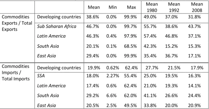
From Table 1, we can notice that the export and import dependence on commodities of these countries decreased over time but, in 2008, commodities were still accounting for more than 31.8% of the exports and 17.9% of the imports. Huge differences can be highlighted across regions, Sub-Saharan African countries and Latin American countries being significantly more concentrated on commodity exports than Asian countries. Regarding imports, Asian countries are however importing a larger share of commodities in their total imports than the other developing countries.
Table 1.Descriptive statistics on the full sample
Mean Min Max Mean
1980 Mean 1992 Mean 2008 Commodities Exports / Total Exports Developing countries 38.6% 0.0% 99.9% 49.0% 37.0% 31.8% Sub Saharan Africa 46.7% 0.0% 99.7% 55.7% 38.6% 43.7%
Latin America 46.3% 0.4% 97.9% 57.4% 46.8% 37.1% South Asia 20.1% 0.1% 68.5% 42.3% 15.2% 15.3% East Asia 29.4% 0.0% 99.9% 35.4% 36.7% 17.1% Commodities Imports / Total Imports Developing countries 19.9% 0.62% 62.4% 27.7% 21.5% 17.9% SSA 18.0% 2.27% 55.4% 25.0% 19.5% 16.3% Latin America 17.4% 0.6% 62.4% 21.0% 19.3% 14.1% South Asia 29.2% 6.6% 62.0% 41.1% 26.6% 24.4% East Asia 20.5% 2.5% 49.5% 33.8% 20.0% 20.9%
10 The price level and volatility of imported commodities should affect all the developing countries given that the degree of reliance on commodities of the imports is relatively homogeneous across countries. However, the degree of dependence of exports on commodities ranges between almost zero and 100% according to the country and therefore, the incidence of variations in commodity export prices might be mostly interesting to study in large commodity exporter countries. For the analysis of the export commodity side, we therefore follow Bleaney and Greenaway (2001) and focus on a sub-sample of developing countries where primary products account largely in their exports. On average over the period 2000-2008, primary products accounted for more than 60% of the exports of these countries. The 34 countries retained are listed in Annex 6 and the corresponding descriptive statistics are provided in Annex 7.
Following Deaton and Miller (1999) and Dehn (2000), we construct, for each developing country in our sample, a country-specific index of commodity prices that geometrically weight together the international prices of 41 commodities, using common international prices but fixed individual country weights. The country-specific commodity import price indices are therefore calculated such that:
∏
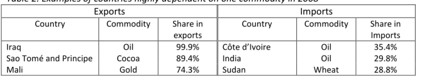
= = 41 1 , , , c w t c t i c i p Iwhere pc,t is the international price of commodity c in year t. The weight wi,c is an average over the period 2000 to 2008 of the share of commodity c imports in total commodity imports of country i. The weight of each commodity is then held constant over time. The country-specific commodity export price indices are calculated in a similar way, the weight w being for exports instead of imports. Forty-one commodities are distinguished and their international prices are drawn from IMF data. Among agricultural commodities, we consider: bananas, barley, beef, cocoa, coffee, cotton, groundnuts, hides, lamb, maize, olive oil, orange, palm oil, pork, poultry, rice, rubber, salmon, sawnwood, shrimp, soybean oil, soybean, sugar, sunflower oil, tea, wheat, wool corse, wool fine; among minerals: aluminium, copper, iron ore, lead, nickel, tin, uranium, zinc, gold, silver and among energetic commodities: coal, gas and oil. The share of these commodities in the imports and exports of each country are obtained from WITS with the SITC 2 classification disaggregated over 4 digits. Table 2 gives some illustrative examples of countries largely dependent on one given commodity.
Table 2. Examples of countries highly dependent on one commodity in 2008
Exports Imports
Country Commodity Share in exports
Country Commodity Share in Imports
Iraq Oil 99.9% Côte d’Ivoire Oil 35.4%
Sao Tomé and Principe Cocoa 89.4% India Oil 29.8%
Mali Gold 74.3% Sudan Wheat 28.8%
The country-specific price indices are then deflated by the unit value index of advanced economies exports, taken from the International Financial Statistics of the IMF. As first evidence, the relationships between these country-specific commodity price indices and our variable of interest, namely tax revenue are depicted graphically in Annex 8. According to these correlations, the prices of both imported and exported commodities are positively associated with tax revenue.
11 The volatility of commodity prices is assessed through two distinct measures. The standard deviation is the most common indicator of variability (Mendoza, 1997, for terms of trade volatility or Aghion et al., 2009, for exchange rate volatility, among others). We therefore firstly measure commodity price volatility as the standard deviation of the first-difference of the deflated country-specific price indices. The volatility of the composite price indices which is calculated can however under-estimate the volatility really faced by a country. Indeed, the variations of two commodity prices in opposite directions can be neutralized within the price index, resulting in only a low volatility of the price index. To avoid this compensation mechanism and asses the total volatility which is affecting countries, we propose a second measure of volatility. We compute the volatility of each of the 41 commodity prices by taking the standard deviation of the first-difference of the deflated prices. We then compute the country-specific commodity price volatility as the weighted average of these 41 price volatilities. The weights for each commodity are those used to construct the country-specific price indices.
In order to test the theoretical mechanisms identified above, we build a short-run volatility measure (used for import prices) based on monthly data for each year, and a medium-run volatility measure (used for export prices), computed using yearly data over five-year rolling windows (following Bekaert et al., 2006).
To assess the impact on public revenues of variations in both the levels of commodity prices and the volatility of these prices, the basic estimated equation, for the import side, is of the following form:
t i i t i M t i M t i t i
I
X
T
,=
α
+
β
1log(
,)
+
β
2log(
σ
,)
+
'
,β
3+
µ
+
ε
,This equation will be also estimated separately for each imported commodity category (agriculture, minerals and energy).5 However, given the high concentration of commodity exports on a few products at the country level, this disaggregation of exports price into three categories is not feasible.
For the sub-sample of large commodity exporting countries, the estimated equation will be:
t i i t i X t i X t i t i
I
X
T
,=
α
+
δ
1log(
,)
+
δ
2log(
σ
,)
+
'
,δ
3+
µ
+
ε
,where i and t are country and time period indicators respectively, the dependent variable T is the tax revenue as part of GDP and will be either total government revenue, excluding grants, or one of the disaggregated tax revenue category (income taxes, domestic indirect taxes, trade taxes).
I
iM,t andI
iX,tare the commodity price indices for imports and exports respectively whereas
σ
iM,t andσ
iX,t represent the commodity price volatility. Following Collier and Goderis (2007), to allow the effect of5
A more disaggregated approach (product by product) is theoretically appealing, but unfortunately not feasible for two main reasons: ii) individual commodity prices variations correspond to a common shock for all countries, already captured by time fixed effects, ii) a simultaneous test of the different product prices would imply too many right hand side variables (with strong correlations between them).
12 import and export price volatility to be larger for countries with higher imports and exports, the country-specific volatility of imported and exported commodities were weighted respectively by the share of imports and exports in the countries’ GDP.
The vector X captures other explanatory variables affecting tax revenue. Drawing on the empirical literature that models the share of tax revenues in GDP (Adam et al., 2001; Khattry and Rao, 2002; Keen and Lockwood, 2010), we include the following variables as control. The lagged dependent variable controls for the persistence of tax revenues. The GDP per capita is a proxy for the tax base and the tax administration capacity, higher level of per capita income is usually found to be positively related to domestic tax revenues. The structure of the economy is proxied by the share of agriculture in GDP usually negatively associated with the domestic tax revenues over GDP ratio (agriculture, in particular the subsistence sector is less easily taxed than industry and services). The degree of openness should be positively associated with domestic tax performance given that, in developing countries, a large part of the taxes are collected at the borders. Higher inflation is supposed to reduce domestic tax yields according to the Tanzi Olivera effect. Theory suggests that foreign aid may have some impact on public revenues; recent evidence shows that foreign aid (especially grants) has been associated with increases in tax revenues (Brun et al., 2007; Clist and Morrissey, 2011). We also include the proportion of the population under 14 years, the tax ratio usually being increasing with the number of dependent in the population. All these variables are from the World Development Indicator (WDI) database.
The OLS estimator becomes inconsistent because the lagged level of tax revenue is correlated with the error term due to the presence of country fixed effects (Nickell, 1981). One way to handle these issues is to use the Generalized Method of Moments (GMM) technique (Blundell and Bond, 1998). The System-GMM estimator combines, in a system, first-difference equations, where the right-hand-side variables are instrumented by lagged levels of the series with an additional set of equations in levels, using lagged first differences of the series as instruments. We will also present the AR(1), AR(2) and Hansen tests to ascertain that the econometric results are consistent.
4. Results
4.1. The effect of commodity import price level and volatility
The results with the GMM-System estimator are presented in Table 3 (first measure of volatility) and Table 4 (second measure of volatility). The first two columns present the results for the total government revenue, excluding foreign aid, whereas in the six subsequent columns, the results represent the three different categories of taxes, namely income taxes, domestic indirect taxes and taxes on international trade. For each dependent variable, we use successively the aggregated price index (columns 1, 3, 5 and 7) and disaggregated price indexes (columns 2, 4, 6 and 8)
Increased prices on the imported commodities appear to lead to more taxes being collected. The effect is non-negligible, an increase of 10% in the price index leading to a rise of 0.36 percentage points6 in the total revenue ratio over GDP. The channel of this positive impact is difficult to identify
6
13 since none of the categories of taxes appear to be significantly positively affected by increased import prices. This weakly significant effect can be explained by the presence of tax exemptions (either tariff rate decreases or indirect consumption tax rate decreases) in times of high prices and therefore even though the tax base is higher (because of the increased price of imports) it does not necessarily translate into higher taxes being collected. Looking at the disaggregated effects by category of commodities (agricultural, minerals and energy), we can notice a strong heterogeneity of results. The price of agricultural products has a positive impact on total tax revenues, but this impact cannot be identified among disaggregated revenues. Trade taxes are positively affected by energy prices, but the impact on total revenues is not significant. Lastly, energy prices exhibit no impact on total revenues or on any specific tax component.
Regarding the short-run volatility of the prices of these imported commodities, we can see that it is leading to decreased tax revenues. The result originates from domestic consumption taxes and taxes on international trade which are negatively affected by the volatility of the commodity import prices. We may notice that international trade taxes are more vulnerable than consumption taxes to price volatility (the negative marginal impact being roughly twice as large, see columns 5 and 7). This negative effect of volatility can be explained by the existence of asymmetries where tax exemptions on imported goods are granted in times of price spikes resulting in lower taxes being collected but during times of low prices, tax rates are not increased and thus do not result in more taxes being collected. The negative impact of short-term volatility on tax revenues is hardly identified when commodities are disaggregated; the impact is identified either only on total taxes (energy) or on disagregated taxes (minerals and agriculture).
The control variables included in the model exhibit the expected sign. The lagged dependent variables and imports are significantly positively associated with tax revenues. The value added in the agriculture sector is inducing decreased consumption taxes being collected and so does the GDP. The remaining control variables are non-significant. AR(1), AR(2) and Hansen tests confirm the adequacy and the validity of our instruments.
With this first measure of volatility, the variations in the price of different commodities can be compensated, the commodity price volatility being therefore lower than what is really faced by governments. Estimations using an alternative measure of the commodity price volatility are given in Table 4.
The results presented in Table 4 exhibit only few differences compared to those obtained using the conventional measure of volatility. The negative impact of import price volatility on tax revenues is significant at the 1% level and originates from consumption and international trade taxes, confirming our previous result. Again, the detrimental effect of volatility is larger for international trade taxes than for consumption taxes. Differences on estimations using disaggregation of tax revenues price indexes are only minor. The negative impact of agricultural price volatility is stronger than previously (significant for total tax revenues) while the impact of energy price volatility is no longer significant. From these disaggregated measures of volatility we can also remark that the largest marginal negative impact of import price volatility appears to originate from agricultural products.
14 VARIABLES Tax Revenue
(%GDP) Tax Revenue (%GDP) Income Tax (%GDP) Income Tax (%GDP) Consumption Taxes (%GDP) Consumption Taxes (%GDP) International Trade Taxes (%GDP) International Trade Taxes (%GDP) (1) (2) (3) (4) (5) (6) (7) (8)
Commodity import price index 3.792*** 0.392 0.0788 0.522
(1.203) (0.556) (0.456) (0.554)
Commodity import price volatility -0.388*** -0.101 -0.128** -0.260**
(0.125) (0.0831) (0.0545) (0.103)
Minerals import price index 1.049 0.471 1.027* -0.379
(1.626) (0.872) (0.542) (0.805)
Minerals import price volatility -0.0482 0.00466 -0.102** -0.0271
(0.134) (0.0552) (0.0443) (0.0744)
Energy import price index 0.346 -0.274 0.00592 -0.0832
(0.648) (0.379) (0.255) (0.433)
Energy import price volatility -0.0954* 0.0135 -0.00256 -0.0343
(0.0556) (0.0222) (0.0277) (0.0353)
Agricultural import price index 3.560 1.132 0.0432 1.882
(2.188) (1.189) (0.856) (1.693)
Agricultural import price volatility -0.193 -0.235** -0.163* -0.218
(0.189) (0.110) (0.0924) (0.147)
Lagged dependent variable 0.680*** 0.682*** 0.840*** 0.828*** 0.954*** 0.973*** 0.889*** 0.828*** (0.0883) (0.0969) (0.0470) (0.0606) (0.0634) (0.0589) (0.205) (0.261) Imports (%GDP) 0.0618** 0.0559** 0.0210** 0.0222** 0.0214* 0.0255*** 0.0281** 0.0271**
(0.0270) (0.0284) (0.00843) (0.00881) (0.0128) (0.00899) (0.0110) (0.0129) Population below 14 0.0107 -0.000149 0.0507 0.0564 -0.0282 -0.00825 0.0245 0.0567
(0.0934) (0.111) (0.0351) (0.0505) (0.0433) (0.0422) (0.0530) (0.0688) Aid per capita 0.00340 0.00443 0.00366 0.00370 -0.00506 -0.00744*** 0.00924 0.00845 (0.00822) (0.00913) (0.00412) (0.00521) (0.00311) (0.00273) (0.00594) (0.00700) GDP (log) 0.918 0.937 1.417** 1.648* -0.414 -0.314 0.486 0.965 (1.902) (2.220) (0.609) (0.922) (0.804) (0.887) (1.216) (1.663) Agriculture (%GDP) -0.0371 -0.0372 0.0592* 0.0715 -0.0175 -0.0144 0.0233 0.0421 (0.0915) (0.101) (0.0314) (0.0462) (0.0364) (0.0394) (0.0539) (0.0729) Observations 1,907 1,907 1,578 1,578 1,734 1,734 1,737 1,737 Nb of countries 90 90 88 88 88 88 88 88 Nb of instruments 23 27 23 27 19 23 15 19
AR(1) Test : p-val 0.000 0.000 0.000 0.000 0.000 0.000 0.006 0.021
AR(2) Test : p-val 0.568 0.588 0.410 0.413 0.179 0.143 0.537 0.554
Hansen Test : p-val 0.286 0.206 0.682 0.631 0.368 0.550 0.220 0.157
Note: Robust standard errors in brackets. ***, ** and * denote significance at the 1%, 5% and 10% levels respectively. Constant and country fixed effects included but not reported. Two-step GMM using the Windmeijer (2005) correction with collapsed instruments. The price indices and volatility, the population below 14 and the agricultural value-added are treated as exogenous whereas imports and the lagged dependent variable are considered as predetermined and the level of GDP per capita and of aid per capita as endogenous. The number of lags used to instrument variables varies from one dependent variable to another. In the four first columns, predetermined
variables are instrumented with their 1st to 4th-order lagged values and endogenous variables by 2nd to 4th-order lagged values. In columns 5 and 6, predetermined variables instrumented with 1st to 3rd-order lags and
15 VARIABLES Tax Revenue (%GDP) Tax Revenue (%GDP) Income Tax (%GDP) Income Tax (%GDP) Consumption Taxes (%GDP) Consumption Taxes (%GDP) International Trade Taxes (%GDP) International Trade Taxes (%GDP) (1) (2) (3) (4) (5) (6) (7) (8)
Commodity import price index 4.538*** 0.692 0.519 0.836
(1.324) (0.713) (0.506) (0.643)
Commodity import price volatility -0.340*** -0.0771 -0.130** -0.181**
(0.131) (0.0705) (0.0657) (0.0863)
Minerals import price index -0.394 0.289 1.008 -1.713
(1.836) (1.037) (0.663) (1.638)
Minerals import price volatility 0.107 0.0297 -0.0865** 0.0910
(0.119) (0.0575) (0.0383) (0.125)
Energy import price index 0.103 -0.230 -0.0356 -0.222
(0.665) (0.405) (0.265) (0.549)
Energy import price volatility -0.0498 0.0110 0.00821 0.0122
(0.0600) (0.0228) (0.0306) (0.0443)
Agricultural import price index 6.024** 1.322 0.808 4.108
(2.826) (1.639) (1.194) (2.975)
Agricultural import price volatility -0.410* -0.146 -0.193** -0.384*
(0.225) (0.134) (0.0944) (0.220)
Lagged dependent variable 0.671*** 0.677*** 0.823*** 0.820*** 0.963*** 0.978*** 0.809*** 0.888***
(0.0954) (0.103) (0.0528) (0.0662) (0.0590) (0.0580) (0.226) (0.282)
Imports (%GDP) 0.0632** 0.0586* 0.0189** 0.0205** 0.0205 0.0268*** 0.0257** 0.0277**
(0.0285) (0.0315) (0.00849) (0.0101) (0.0134) (0.00971) (0.0110) (0.0140)
Population below 14 0.0225 0.00671 0.0537 0.0446 -0.0146 -0.00312 0.0308 0.0978
(0.107) (0.125) (0.0408) (0.0533) (0.0440) (0.0460) (0.0542) (0.107)
Aid per capita 0.00264 0.00769 0.00327 0.00291 -0.00507* -0.00588** 0.00685 0.0109
(0.00862) (0.00887) (0.00427) (0.00552) (0.00267) (0.00251) (0.00602) (0.00767) GDP (log) 1.186 1.409 1.442** 1.422 -0.201 -0.0758 0.306 2.042 (2.152) (2.522) (0.732) (1.034) (0.825) (0.979) (1.304) (2.622) Agriculture (%GDP) -0.0303 -0.0157 0.0572 0.0586 -0.0101 -0.00385 0.00973 0.0887 (0.0972) (0.113) (0.0364) (0.0524) (0.0368) (0.0439) (0.0559) (0.116) Observations 1,907 1,907 1,578 1,578 1,734 1,734 1,737 1,737 Nb of countries 90 90 88 88 88 88 88 88 Nb of instruments 23 27 23 25 19 23 15 19
AR(1) Test : p-val 0.000 0.000 0.000 0.000 0.000 0.000 0.013 0.020
AR(2) Test : p-val 0.585 0.580 0.413 0.409 0.166 0.129 0.574 0.407
Hansen Test : p-val 0.270 0.219 0.660 0.643 0.289 0.548 0.124 0.236
16 Results regarding the import prices may be summed up as follows. First, a positive impact of the commodity price level on tax revenues; second a negative impact of short-term volatility, channeled through reduced consumption and trade taxes; third, a larger vulnerability of international trade taxes to price volatility (compared to consumption taxes).
4.2. The effect of exported commodity price level and volatility
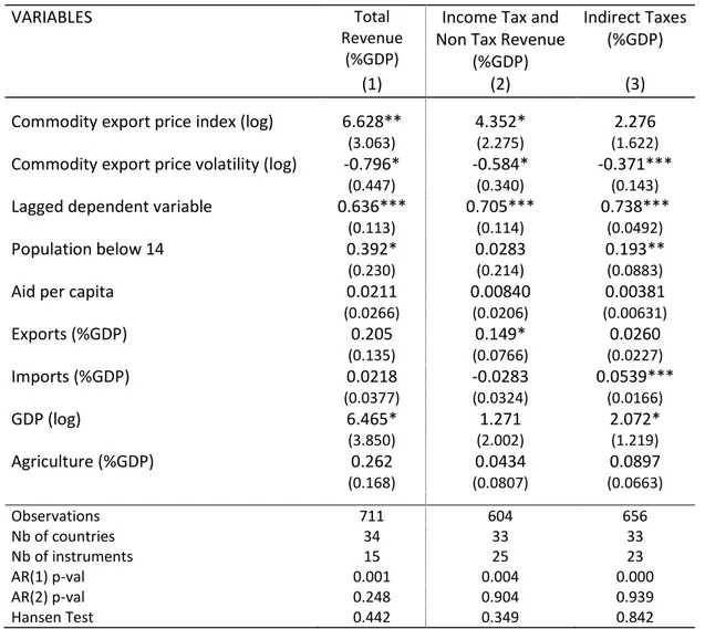
Turning now to the export side, Table 5 reports the estimation results with the System-GMM estimator and our first measure of commodity export price volatility. Both the level and the medium-run volatility of commodity export prices appear to significantly influence total public revenue (column 1). Higher prices for exported commodities have significantly large positive impacts on the total revenue collected in exporting countries. Indeed, an increase of 10% in the price index will lead to a rise of 0.66 percentage points in the total revenue ratio over GDP. For the mean level of total revenue in our sample of exporting countries (18.3% of GDP), this 10% increase in the commodity export prices could lead to a rise of about 3.5% of total revenue.
However, increased volatility of these international prices moves significantly the revenue ratio in the opposite direction. Therefore, a country with a one standard deviation greater level of volatility than the mean, which corresponds to a rise of 79.5%, will mobilize 0.47 percentage point7 less tax revenue over GDP than the sample average. We therefore provide evidence that volatile prices for exported commodities are negatively affecting tax revenues.
The control variables exhibit the expected signs with a larger dependent population and a higher level of GDP per capita being positively and significantly associated with total government revenue over GDP. Moreover, the AR(1), AR(2) and Hansen Tests confirm that our estimation results are reliable.
The subsequent columns (2 and 3) present the effects on the different components of government revenue that might be affected by variations in exported commodity prices. In column 2, the dependent variable is the sum between the non-tax revenue and the income tax revenue. Indeed, a substantial effect of export prices on revenue can happen either through the non-tax revenue or through the income tax revenue depending on which arrangement the countries did set in their mining or petroleum investment codes (payments through dividends with a state participation in the companies, through royalties or only through profit taxes). Given the large variety of systems across countries, we retain as dependent variable the sum of non-tax and income tax revenues to include any situation prevalent in our sample of countries.
The identified positive effect of commodity export prices on tax revenues seem to originate in the joint category income and non-tax revenue. A rise in the commodity export prices increases the collection of these revenues whereas export price volatility negatively affects them. An enhancement of export prices leads to higher tax revenues, as developed in section 2.1, through both the price and tax rate effects and the macroeconomic effects of increased growth and investments. The volatility of terms of trade has been however found to induce less foreign investment (Blattman, 2007) and
7
17 therefore this adverse macroeconomic effect can lead to less tax revenues being collected. In column 3, as expected, there is no evidence of significant impact of the level of exported commodity prices on indirect taxes revenues. Nevertheless, medium-run volatility is detrimental to these indirect tax revenues (presumably through a revenue channel).
Table 5. Impact of exported commodity price level and volatility (System-GMM – 1st indicator of volatility)
VARIABLES Total
Revenue (%GDP)
Income Tax and Non Tax Revenue
(%GDP)
Indirect Taxes (%GDP)
(1) (2) (3)
Commodity export price index (log) 6.628** 4.352* 2.276
(3.063) (2.275) (1.622)
Commodity export price volatility (log) -0.796* -0.584* -0.371***
(0.447) (0.340) (0.143)
Lagged dependent variable 0.636*** 0.705*** 0.738***
(0.113) (0.114) (0.0492)
Population below 14 0.392* 0.0283 0.193**
(0.230) (0.214) (0.0883)
Aid per capita 0.0211 0.00840 0.00381
(0.0266) (0.0206) (0.00631) Exports (%GDP) 0.205 0.149* 0.0260 (0.135) (0.0766) (0.0227) Imports (%GDP) 0.0218 -0.0283 0.0539*** (0.0377) (0.0324) (0.0166) GDP (log) 6.465* 1.271 2.072* (3.850) (2.002) (1.219) Agriculture (%GDP) 0.262 0.0434 0.0897 (0.168) (0.0807) (0.0663) Observations 711 604 656 Nb of countries 34 33 33 Nb of instruments 15 25 23 AR(1) p-val 0.001 0.004 0.000 AR(2) p-val 0.248 0.904 0.939 Hansen Test 0.442 0.349 0.842
Note: Robust standard errors in brackets. ***, ** and * denote significance at the 1%, 5% and 10% levels respectively. Constant and country fixed effects included but not reported. Two-step GMM using the Windmeijer (2005) correction with collapsed instruments. The price indices and volatility, the population below 14 and the agricultural value-added are treated as exogenous whereas imports, exports and the lagged dependent variable are considered as predetermined and the level of GDP per capita and of aid per capita as endogenous. The number of lags used to instrument variables varies from one dependent variable to another. In the first column, predetermined variables are instrumented with their 1st-order lagged values and endogenous variables by their 2nd-order lagged values. In column 2, predetermined variables instrumented with 1st to 3rd-order lags and endogenous variables with 2nd to 4th-order lags. In column 3, predetermined variables instrumented with 1st to 3rd-order lags and endogenous variables with 2nd to 3rd-order lags.
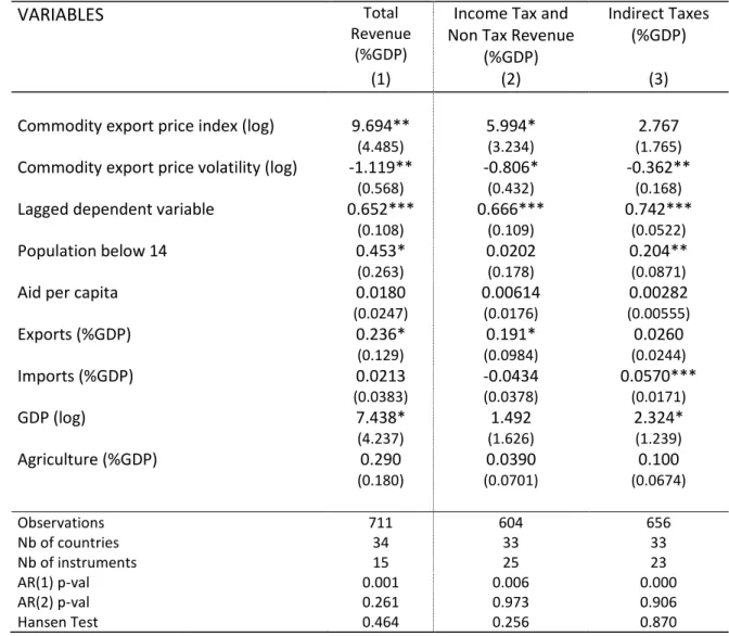
In Table 6, we test the robustness of these results by using our alternative measure of commodity export price volatility. The first column of the Table reports the estimation for total government revenue as a share of GDP, confirming our previous result that the price volatility of export
18 commodities is detrimental for tax revenue collection. The effect appears to be even larger with this second indicator of the price volatility than with the previous one given that, as explained previously, there is no compensation between the volatilities of different commodities in this second indicator. The marginal impact stands at -1.119, which corresponds to a loss of 0.65 percentage point of revenue when the price volatility increases of one standard deviation.
Table 6. Impact of exported commodity price level and volatility (System-GMM –2nd indicator of volatility)
VARIABLES Total
Revenue (%GDP)
Income Tax and Non Tax Revenue
(%GDP)
Indirect Taxes (%GDP)
(1) (2) (3)
Commodity export price index (log) 9.694** 5.994* 2.767
(4.485) (3.234) (1.765)
Commodity export price volatility (log) -1.119** -0.806* -0.362**
(0.568) (0.432) (0.168)
Lagged dependent variable 0.652*** 0.666*** 0.742***
(0.108) (0.109) (0.0522)
Population below 14 0.453* 0.0202 0.204**
(0.263) (0.178) (0.0871)
Aid per capita 0.0180 0.00614 0.00282
(0.0247) (0.0176) (0.00555) Exports (%GDP) 0.236* 0.191* 0.0260 (0.129) (0.0984) (0.0244) Imports (%GDP) 0.0213 -0.0434 0.0570*** (0.0383) (0.0378) (0.0171) GDP (log) 7.438* 1.492 2.324* (4.237) (1.626) (1.239) Agriculture (%GDP) 0.290 0.0390 0.100 (0.180) (0.0701) (0.0674) Observations 711 604 656 Nb of countries 34 33 33 Nb of instruments 15 25 23 AR(1) p-val 0.001 0.006 0.000 AR(2) p-val 0.261 0.973 0.906 Hansen Test 0.464 0.256 0.870
Note: See the notes of Table 5.
The positive relationship between commodity export prices and revenue also holds, which is consistent with the results established by Medina (2010) with time-series analyses for Latin American and high-income commodity-exporting countries and by Kumah and Matovu (2007) for Russia and three central Asian countries. These effects robustly arise from one component of government revenue, namely income taxes and non-tax revenues.
Globally, the results displayed in Table 5 and 6 illustrate an additional important aspect of the impact of the commodity export price volatility that has never (to our knowledge) received attention: price volatility of exported commodities leads to decreased tax revenues.
19 5. Conclusion and policy implications
In this paper we estimated, on a sample of 90 developing countries over the period 1980-2008, the impact on fiscal revenues of commodity price volatility rather than focusing only on price levels. We used disaggregated data on tax revenues (income tax, consumption tax and international trade tax) and on commodity prices (agricultural products, minerals and energy) in order to identify the transmission channels between world commodity prices and public finance variables.
Our analysis suggests that tax revenues in developing countries increase with the prices’ rise of either imported or exported commodities. For imported commodities this increase in fiscal revenue is due to more tariffs being collected but, because of the numerous tax exemptions granted in times of high prices, the positive impact on tax revenue may not always happen. In our sub-sample of large commodity-exporting economies, the effect is more straightforward: the tax revenue increases due to an export price spike are originating in more profit tax and non-tax revenues, such as dividends or royalties, being collected on companies which are producing primary products.
We find however robust evidence that international commodity price instability, both for imported and exported products has an adverse effect on tax revenues in developing countries. Import commodity price short-term volatility hurts indirect tax revenues while, export price medium-run volatility affects both direct taxes (income tax and non-tax revenues) and indirect tax (consumption tax and trade tax).
These results suggest several policy recommendations. First, this highlights further the importance of finding ways to both limit this international price volatility (through world markets regulation for instance) and manage the macroeconomic effects of the price instability (through national policies). Second, the shift from trade tax to consumption taxes could be expected to reduce the vulnerability of tax revenues to commodity price level and volatility. Third, the negative effect of import price volatility being partly due to the frequent use of tariff or tax exemptions on some primary products, the adequacy of these temporary tax exemptions should deserve further examination.
20 6. References
Adam, C. S., D.L. Bevan and G. Chambas (2001) ‘Exchange rate regimes and revenue performance in Sub-Saharan Africa,’ Journal of Development Economics, 64(1), pp.173-213.
Aghion, P., P. Bacchetta, R. Rancière and K. Rogoff (2009) ‘Exchange rate volatility and productivity growth: The role of financial development’, Journal of Monetary Economics, 56: 494-513.
Akiyama, T., J. Baffes, D. F. Larson and P. Varangis (2003) ‘Commodity Market Reform in Africa’, World Bank Policy Research Working Paper 2995
Bekaert, G., C. R. Harvey and C. Lundblad (2006) ‘Growth volatility and financial liberalization’, Journal of International Money and Finance, 25, pp.370-403.
Blattman, C., J. Hwang and J. G. Williamson (2007) ‘Winners and Losers in the Commodity Lottery: The Impact of Terms of Trade Growth and Volatility in the Periphery 1870–1939,’ Journal of Development Economics, 82 (1), pp.156-79.
Bleaney, M. and D. Greenaway (2001) ‘The impact of terms of trade and real exchange rate volatility on investment and growth in sub-Saharan Africa,’ Journal of Development Economics, 65(2), pp.491-500.
Blundell, R., and S. Bond (1998) ‘Initial conditions and moment restrictions in dynamic panel data models,’ Journal of Econometrics, 87, pp.115-143.
Brun, J-F, Chambas, G., Guérineau, S., 2007, Aide et mobilisation fiscale dans les pays en développement, Rapport thématique, JUMBO, n°21, Agence Française de Développement.
Cashin, P., C. McDermott, C. John and C. Pattillo (2004) ‘Terms of trade shocks in Africa: are they short-lived or long-lived?,’ Journal of Development Economics, 73(2), pp. 727-744.
Cashin P., C. McDermott, and A. Scott (2002). ‘Booms and Slumps in World Commodity Prices,’ Journal of Development Economics, 69, pp.277– 296.
Clist, P. and O. Morrissey (2011) ’Aid and Tax Revenue: Signs of a Positive Effect Since the 1980s,’ Journal of International Development, 23(2), pp.165-180.
Collier, P. and B. Goderis (2007) ‘Commodity Prices, Growth, and the Natural Resource Curse: Reconciling a Conundrum’, CSAE Working Paper No 2007-15.
Collier, P., J. W. Gunning and associates (1999) ‘Trade Shocks in Developing Countries.’ Vol. 1: Africa, Vol. 2: Asia and Latin America, Oxford: Oxford University Press.
Deaton, A. (1999) ‘Commodity Prices and Growth in Africa," Journal of Economic Perspectives, 13(3), 23-40.
Deaton, A. and G. Laroque (1992). ‘On the Behaviour of Commodity Prices,’ Review of Economic Studies, 59(1), pp 1-23.
Deaton, A. and R. Miller (1996). ‘International Commodity Prices, Macroeconomic Performance and Politics in Sub-Saharan Africa,’ Journal of African Economies, 5(3), pp. 99-191.
Dehn, J. (2000) ‘Commodity Price Uncertainty in Developing Countries,’ World Bank Policy Research Working Paper No. 2426.
FAO, 2009, Country Responses to Food Security Crisis: Nature and Preliminary Implications of the Policies Pursued, Initiative on soaring food prices, 31p.
Guillaumont, P. (1987) ‘From export instability effects to international stabilization policies,’ World Development, 15(5), pp. 633-643.
21 International Monetary Fund (2008) ‘Food and Fuel Prices—Recent Developments, Macroeconomic
Impact, and Policy Responses An Update,’ IMF Policy Paper.
Keen, M. and B. Lockwood (2010) ‘The value added tax: Its causes and consequences’ Journal of Development Economics, 92(2), pp.138-151.
Khattry, B. and M.J. Rao (2002) “Fiscal Faux Pas?: An Analysis of the Revenue Implications of Trade Liberalization”, World Development 30(8), pp.1431-1444.
Kose, M. A., and R.G. Riezman (2001). ‘Trade shocks and macroeconomic fluctuations in Africa,’ Journal of Development Economics, 65(1), 55-80.
Kumah, F. Y. and J. Matovu (2007) ‘Commodity Price Shocks and the Odds on Fiscal Performance: A Structural Vector Autoregression Approach’ IMF Staff Papers, 54(1), pp. 91-112.
Leenhardt, B. (2005) ‘Fiscalité pétrolière au sud du Sahara : la répartition des rentes,‘ Afrique contemporaine, 4(216).
Larson, D. F., P. Varangis and N. Yabuki (1998) ‘Commodity Risk Management and Development’ World Bank Policy Research Paper No. 1963.
Medina, L. (2010) ‘The Dynamic Effects of Commodity Prices on Fiscal Performance in Latin America,’ IMF Working Papers No.10/192.
Mendoza, E. G. (1997) ‘Terms-of-trade uncertainty and economic growth’, Journal of Development Economics, vol.54 pp.323-356.
Nickell, S. (1981) ‘Biases in dynamic models with fixed effects,’ Econometric, 49, pp. 1417–1426. Pindyck, R.S. and J.J. Rotemberg (1990) ‘The Excess Co-movement of Commodity Prices,’ Economic
Journal, 100(403), pp. 1173-89.
Raddatz, C. (2007) ‘Are external shocks responsible for the instability of output in low-income countries?,’ Journal of Development Economics, 84(1), pp.155-18.
Ramey, G. and V.A. Ramey (1995) ‘Cross-Country Evidence on the Link between Volatility and Growth,’ American Economic Review, 85(5), pp. 1138-51.
Subervie,J. (2008) ‘The Variable Response of Agricultural Supply to World Price Instability in Developing Countries,’ Journal of Agricultural Economics, 59(1), pp.72-92.
Talvi, E. and C.A. Vegh (2005) ‘Tax base variability and procyclical fiscal policy in developing countries,’ Journal of Development Economics, 78(1), pp. 156-19.
Varangis, P. and D.F. Larson (1996) ‘Dealing with Commodity Price Uncertainty,’ World Bank Policy Research Working Paper No. 1667.
Windmeijer, F. (2005) ‘A finite sample correction for the variance of linear efficient two-step GMM estimators,’ Journal of Econometrics, 126(1), pp. 25-51.
22 7. Annexes
23 Annex 2: Trade based policy measures (FAO, 2009)
24 Annex 3: Synthesis of commodity price effects on public revenues
Theoretical mechanisms on import prices
High commodity prices (Effect: < or > 0 ?) Volatile commodity prices (Effect: < 0)
Microeconomic effects
Trade and consumption taxes ( <> 0 ?) Price effect: > 0
Tax rate effect: < 0
(Tax exemptions on food and oil imports) Volume effect: < 0 / = 0
(if non traded substitutes, less taxed)
Trade and consumption taxes ( < 0) Price effect: = 0 (ad valorem tax) Tax rate effect: < 0
(asymmetry of tax exemptions) Volume effect: < 0 = 0
(if less volatile substitutes, partly non tradable, less taxed)
Macroeconomic effects
Income taxes ( < 0) Indirect taxes (< 0) Revenue effect: < 0 < 0 Real exchange rate effect = 0 = 0
Income taxes (< 0) Indirect taxes (< 0) Growth volatility effect < 0
(GDP growth volatility – lower GDP growth )
Theoretical mechanisms on export prices
High commodity prices (Effect: > 0) Volatile commodity prices (Effect: <> 0 ?)
Microeconomic effects
Trade and profit taxes, royalties ( > 0) Price effect: > 0
Tax rate effect: > 0 (taxation of windfall gains) Volume effect: > 0 / = 0 (if supply response)
Trade and profit taxes, royalties (> 0) Price effect: = 0 (ad valorem tax)
> 0 (progressive / margin tax) Tax rate effect: > 0
(asymmetry of ad hoc taxes ) Volume effect: < 0 / = 0
(if non traded & less volatile substitutes, less taxed)
Macroeconomic effects
Income taxes ( > 0) Indirect taxes (> 0) Revenue effect: > 0 > 0 Real exchange rate effect < 0 > 0
Income taxes (< 0) Indirect taxes (< 0) Growth volatility effect < 0
25 Annex 4. The 90 developing countries in the sample
Afghanistan, Albania, Algeria, Argentina, Armenia, Azerbaijan, Bangladesh, Benin, Bolivia, Botswana, Brazil, Burkina Faso, Burundi, Cambodia, Cameroon, Cape Verde, Central African Republic, Chile, China, Colombia, Comoros, Cote d'Ivoire, Egypt. Arab Rep., El Salvador, Eritrea, Ethiopia, Fiji, Gabon, Gambia. The, Georgia, Ghana, Guatemala, Guinea, Guinea-Bissau, Honduras, India, Indonesia, Iran. Islamic Rep., Jamaica, Jordan, Kazakhstan, Kenya, Kyrgyz Republic, Lebanon, Lesotho, Madagascar, Malawi, Maldives, Mali, Mauritania, Mauritius, Mexico, Moldova, Mongolia, Morocco, Mozambique, Namibia, Nepal, Nicaragua, Niger, Nigeria, Pakistan, Panama, Papua New Guinea, Paraguay, Peru, Philippines, Rwanda, Samoa, Senegal, Sierra Leone, South Africa, Sri Lanka, Sudan, Suriname,
Swaziland, Syrian Arab Republic, Tajikistan, Thailand, Togo, Tonga, Tunisia, Turkey, Uganda, Ukraine, Uruguay, Venezuela, Vietnam, Yemen, Zambia.
Annex 5. Descriptive Statistics
Variable Obs Mean Std
Dev
Min Max Revenue (%GDP) 1770 19.16 7.962 2.228 54.4 Income Taxes (%GDP) 1483 4.395 2.852 0.105 23.9 Consumption Taxes (%GDP) 1608 5.696 3.169 0.021 21.962 International Trade Taxes (%GDP) 1610 3.813 3.651 0.054 37.1 Commodity import price index (log) 1770 0.536 0.117 0.311 1.168 Agricultural import price index (log) 1770 0.507 0.0622 0.332 0.767 Energy import price index (log) 1770 0.604 0.240 0.270 1.474 Minerals import price index (log) 1770 0.592 0.135 0.288 1.410 Volatility of commodity import prices (log)a 1770 2.605 2.247 0.104 20.880
Volatility of commodity import prices (log)b 1770 4.816 3.465 0.524 31.182
Volatility of agricultural import prices (log)a 1770 2.367 1.699 0.257 16.520
Volatility of agricultural import prices (log)b 1770 3.891 2.457 0.503 20.464
Volatility of energy import prices (log)a 1770 5.955 5.215 0.133 36.840
Volatility of energy import prices (log)b 1770 6.796 5.735 0.143 39.053
Volatility of minerals import prices (log)a 1770 4.709 3.624 0.233 30.203
Volatility of minerals import prices (log)b 1770 5.719 4.498 0.480 45.573
Population below 14 1770 38.918 7.242 13.942 51.771 Aid per capita 1770 47.540 53.263 -40.38 438.24
Imports 1770 39.941 21.710 4.631 147.65
GDP (log) 1770 7.550 0.966 5.227 9.636
Agriculture (%GDP) 1770 23.489 13.999 1.833 68.879 Notes: aVolatility based on the first measure; bVolatility based on the first measure
26 Annex 6. The 34 exporting developing countries
Algeria, Azerbaijan, Belize, Benin, Bolivia, Burkina Faso, Burundi, Cameroon, Costa Rica, Cote d'Ivoire, Ethiopia, Gabon, The Gambia, Ghana, Iran. Islamic Rep., Kazakhstan, Kyrgyz Republic, Mali, Mauritania, Mozambique, Nicaragua, Nigeria, Papua New Guinea, Paraguay, Rwanda, Sierra Leone, Vincent and the Grenadines, Sudan, Syrian Arab Republic, Tajikistan, Uganda, Venezuela, Yemen, Zambia
Note: Angola, Libya, Chad and DRC are excluded from the sample due to the lack of tax revenue data. Botswana is also excluded since diamonds are not included in the IMF International commodity price database.
Annex 7. Descriptive Statistics
Variable Obs Mean Std. Dev. Min Max
Revenue (%GDP) 711 18.335 7.446 2.228 47.193
Income Tax and Non-Tax Revenue (%GDP) 604 9.403 7.266 0.247 37.328 Consumption Taxes (%GDP) 664 5.030 2.598 0.502 17.500 International Trade Taxes (%GDP) 656 3.449 2.441 0.386 16.126 Commodity export price index (log) 711 0.517 0.142 0.274 1.176 Volatility of commodity export price (log)a 711 2.762 2.196 0.090 11.989 Volatility of commodity export price (log)b 711 3.517 2.611 0.159 14.502 Population below 14 711 41.604 5.454 23.671 51.771
Aid per capita 711 48.040 41.638 -8.032 440.874
Exports (%GDP) 711 30.116 17.514 2.525 98.762
Imports (%GDP) 711 36.857 17.112 7.066 100.913
GDP per capita (log) 711 7.317 0.999 5.227 9.595 Agriculture (%GDP) 711 28.281 13.840 4.023 68.879 Notes: aVolatility based on the first measure; bVolatility based on the first measure
27 Annex 8. Correlation between tax revenue and commodity price indices
8.A. Correlation for imported commodities
Source: authors’ calculations
8.B. Correlation for exported commodities in the sub-sample of large commodities exporting countries