HAL Id: halshs-01512716
https://halshs.archives-ouvertes.fr/halshs-01512716
Preprint submitted on 24 Apr 2017
HAL is a multi-disciplinary open access
archive for the deposit and dissemination of sci-entific research documents, whether they are pub-lished or not. The documents may come from teaching and research institutions in France or abroad, or from public or private research centers.
L’archive ouverte pluridisciplinaire HAL, est destinée au dépôt et à la diffusion de documents scientifiques de niveau recherche, publiés ou non, émanant des établissements d’enseignement et de recherche français ou étrangers, des laboratoires publics ou privés.
past disasters influence households’ resilience?
Tebkieta Alexandra Tapsoba
To cite this version:
Tebkieta Alexandra Tapsoba. Poverty, disasters and remittances: do remittances and past disasters influence households’ resilience?. 2017. �halshs-01512716�
SÉRIE ÉTUDES ET DOCUMENTS
Poverty, disasters and remittances: do remittances and past
disasters influence households’ resilience?
Tebkieta Alexandra TAPSOBA
Études et Documents n° 8
April 2017
To cite this document:
Tapsoba T. A. (2017) “Poverty, disasters and remittances: do remittances and past disasters influence households’resilience ? ”, Études et Documents, n° 8, CERDI.
http://cerdi.org/production/show/id/1869/type_production_id/1
CERDI
65 BD. F. MITTERRAND
63000 CLERMONT FERRAND – FRANCE TEL.+33473177400
FAX +33473177428
2
The author
Tebkieta Alexandra Tapsoba PhD Student in Economics
School of Economics and CERDI, University Clermont Auvergne - CNRS, Clermont-Ferrand, France.
E-mail: [email protected]
This work was supported by the LABEX IDGM+ (ANR-10-LABX-14-01) within the program “Investissements d’Avenir” operated by the French National Research Agency (ANR).
Études et Documents are available online at: http://www.cerdi.org/ed
Director of Publication: Grégoire Rota-Graziosi Editor: Catherine Araujo Bonjean
Publisher: Mariannick Cornec ISSN: 2114 - 7957
Disclaimer:
Études et Documents is a working papers series. Working Papers are not refereed, they constitute research in progress. Responsibility for the contents and opinions expressed in the working papers rests solely with the authors. Comments and suggestions are welcome and should be addressed to the authors.
3
Abstract
Using a multi-topic household panel survey conducted in Burkina Faso by the “Institut national de la statistique et de la démographie” (INSD), in 2014, this paper assesses the impact of remittances on poverty in Burkina Faso. To do so, a poverty index is computed using household’s housing characteristics.
Propensity score matching method is used as an empirical strategy, and results show that remittances have a negative impact on poverty.
Another important result is that remittances have a higher impact on the resilience of households, when they have experienced disasters in the past. Therefore, when it comes to natural disasters, these inflows act as an important tool for populations to be more resilient.
Keywords
Poverty, Remittances, Natural Disasters, Resilience, Burkina Faso.
JEL Codes
Introduction
Poverty is an old, but much up to date topic. As a testimony, the first goal of the post 2015 development agenda is aiming to: « End poverty in all its forms everywhere » (UNDP, 2015). Remittances also constitute one of the main concerns of this agenda. In respect of the goal 10, which aims to reduce inequalities within and among countries, one of the targets is to “reduce to less than 3% the transaction costs of migrant remittances and eliminate remittance corridors with costs higher than 5%” (UNDP, 2015). This goal emphasises the importance of remittances especially for developing countries. In fact, they have increased at an impressive rate since the beginning of the 2000s and represent now a major source of foreign inflows in developing countries (Yang & Choi, 2007). According to the (World-Bank), the amount of remittances towards developing countries was around $430 billion in 2014 and $431.6 billion in 2014.
The Sustainable Development Goals then underlines the importance of remittances especially for developing countries, which can be seen as a hedge against poverty. Remittances and poverty have been broadly discussed in the literature, and most of the studies find that remittances reduce poverty in the developing part of the world (Adams, R. & Page, J., 2005) (Acosta, P., Calderon, C., Fajnzylber, P., & Lopez, H., 2008b), (Gupta, Pattillo, C.A., & Wagh, S., 2009).
Using household data of 71 developing countries, (Adams & Page, J, 2005), show that remittances lead to a decrease of 3.5% in the share of poor people. This result is shared by (Acosta, Calderon, P, Fajnzylber, P, & Lopez, H, 2006), for international remittances, with the result that a increase by 1 point in the ratio of remittances to GDP lead to a decrease of 0.4% of poverty rates. (Moises & Kim Donghun, 2011), using a panel of 66 developing countries between 1981 and 2011 show that international remittances reduce poverty, especially for the 10% most poor countries.
On the micro level, (Lopez-Cordova, 2005), in Mexico, (Lokshin & Bontch-Osmolovski, M, 2010) in Nepal, (Gubert, Mesplés-Somps, S, & Lassourd, T, 2010) in Mali, and (Adams & Alfredo, 2013) in Ghana, found that remittances reduce poverty.
Focusing on Burkina Faso, and using the last multi-topic household’s survey conducted in the country in 2014, this paper aims to understand the linkages and particularly assess the impact of remittances on poverty. To our knowledge, this is the first econometrical study applied to this survey.
Despite the fact that this topic has been broadly discussed in the macroeconomics, and microeconomics literature, this paper brings another light on the topic, as we present a new way of measuring poverty.
In the case of Burkina Faso, (Bambio, 2014) found that remittances reduce poverty using low skilled worker emigration in Ivory Coast, and rural-rural move data between 2004 and 2006. As for (Lachaud, 1999), using a national survey on Burkina Faso, remittances tend to reduce the incidence of poverty by 7.2% for rural households, and by 3.2% for urban ones. As majority of papers on poverty, these authors used monetary measures such as income per capita, usually necessary to insure a certain amount of calories per day, expenditures per capita, and so on.
We then chose to compute a poverty index, using housing variables. This index will contribute to the assessment of households’ resilience to natural disasters and climate shocks that some developing countries have to face currently. As remittances and poverty, climate issues occupy an important place in the post 2015 agenda. Hence, the goal 13 aims to “take urgent action to combat climate change and its impacts” (UNDP, 2015). One of the target being to strengthen resilience and adaptive capacity to climate related hazards and natural disasters in all countries.
The rest of the paper is organised as follows: the section 1 consists in addressing the definitions of poverty, and presenting the index computed in this paper; Section 2 presents the scope of the study, some descriptive statistics and the empirical construction of the index; Section 3 is dedicated to the presentation of the methodology, and lastly, Section 4 presents the results and discuss of a potential learning process of households regarding previous shocks.
1. What is poverty?
1.1 : Poverty in the literature
As stated earlier, poverty is an old scourge, fought worldwide, but yet to be solved, especially in developing countries. For (Hartwell, 1972), “Economics is, in essence, the study of poverty”. It cannot be restrained to one definition, but historically, and on the empirical level, poverty has been most commonly defined as a lack of a given amount of income (IPC, 2006).
According to the work of (Ravaillon, 1992), some questions are important when it comes to assessing poverty: “How do we assess individual well-being or “welfare?” “At what level of measured well-being do we say that a person is not poor”, and “how do we aggregate individual indicators of well-being into a poverty measure?”
For the author, the two first questions are referring to an identification problem, of which persons are considered poor, and how poor they are, when the last question is referring to an aggregation problem, and lead to answering of the question how much poverty is there?
When it comes to the measurement of poverty, one common practice is to count the number of people who fall below a poverty line defined in an arbitrary way (Bardhan,P & Udry,C, 1999).
According to (Streeten & al, 1981), poverty entails the non-achievement of basic needs such as “….human needs in terms of health, food, education, water, shelter, transport.”
In this work we chose to compute an index based on the shelter part of these basic needs, in order to measure household’s poverty status, as well to assess their resilience of households when receiving remittances, in the context of climate shocks.
1.2: The poverty index
We based our reflexion on the fact that monetary variables in surveys are usually underestimating poverty due to several factors, such as the fact that household might not include in their response, their annexe activities from informal sector for example. (Filmer, D & Pritchett, L.H) proposed the construction of an index using PCA (Principal Component Analysis) or FA (Factor Analysis) as a proxy of the household’s wealth. This index is an alternative measure to the monetary one, which can easily be biased and non-objective for developing countries (Briand, Anne & Loyal Laré, Amandine, 2013).
In our index, we then focused on housing data, which include the following variables: - The presence of a roof in metal sheet
- The presence of a concrete ground - The presence of drainage system - The presence of a lavatory
- The presence of concrete walls around the house
- The household own a mobile phone in operating condition - The fact that the household lives in a parcelled area
The variables included in this index are referring to the standard of living dimension of the multidimensional poverty index define by UNDP. Multidimensional poverty index is an index of poverty that reflects the deprivation in very rudimentary services and core human functions (Alkire & Santos, M.E, 2010). This index accounts for health, education and standard of living, and was implemented as a result of the millennium objectives indicators (George Owusu; & Francis Mensah, 2013).
The standard of living dimension is referring to aspects such as electricity (household considered deprived if there is no electricity), drinking water (household considered deprived if there is no access to clean drinking water, or clean water is more than 30 minutes of walk away from home), sanitation (deprived if no access to improved toilet), flooring (considered deprived if there is dirt, sand…), cooking fuel (deprived if the
household cook with wood, charcoal), and assets (household considered deprived if it does not own more than one radio, TV, telephone, bike, motorbike, …) (Alkire & Santos, ME, 2010).
The variable of “living in a parcelled area” is included to take into account a growing phenomenon in the country, which is the anarchic and illegal occupation of spaces. This phenomenon can be seen as a result of the growing population in the cities, which inevitably lead to a competition and rise of parcelled areas’ prices.
According to (Vallée & al 2006), outparcelled areas were representing half of sections of Ouagadougou the city capital. They are mainly characterized by barely existence of basic public services and water evacuation systems increasing the risk of being exposed to floods.
Burkina Faso is characterized by Soudano-Sahelian weather with an average annual rainfall between less than 600mm and more than 900mm1. During the past 10 years,
floods have been recurrent in the Niger bassin, consequently in Burkina Faso. For the year 2012 for example, in the provinces of Soum, Oudalan, et Yagha, rainfall recorded for the 30th of September exceed 750 mm where the mean rainfall barely exceeds 600mm a year in the region (sahelian region) (Sighomnou D., 2012). This combined with the fact that the soils where already saturated with water after the rain season beginning in early July-late June. (Hangnon, De Longueville, F, & Ozer, P, 2015) work on extreme precipitations and floods in the main city of Burkina Faso, Ouagadougou for the last ten years show interesting results. In fact, they found that the floods are more the result of unplanned urban growth than any change in the frequency or intensity of extreme rainfall.
We then include this variable in our poverty index, as it also captures the ability of people to leave in safer and therefore parcelled areas.
Ultimately, we think that this index, when computed will give information about the poverty status of the household, and their resilience to natural disasters recorded in the country such as floods and violent wind.
Remittances have been found in the work of (Mohapatra & Ratha, D, 2009) to help household in their preparedness to natural disasters. They show in the case of Ghana, that remittances receiving households tend to live in concrete houses, have electricity, and mobile phones, that play a major part in the preparedness of households to natural disasters. For Burkina Faso, they found that households that receive remittances ten to own concrete houses. We believe that this work can contribute to the debate, by apprehending the resilience of households to natural disasters.
2- The scope of the study / A new poverty indicator
2.1- An overview of the database
This paper took advantage of the most recent household survey conducted in 2014 in Burkina Faso. Burkina Faso is located in sub-Saharan Africa, an area where mass poverty in the world is the most geographically concentrated (Bardhan,P & Udry,C, 1999).
The data are from the “Enquête Multisectorielle Continue” (EMC) of the “Institut National de la Statistique et de la Démographie”, and is a rich database of over 10000 (10800 precisely) households in the 13 regions and the 45 provinces. This survey aimed to understand the characteristics of the households, their employment status, housing, health, education and other socio-economic conditions.
The EMC survey have been implemented to help the institute and the country in updating the annual indicators of the “Stratégie de Croissance Accélélérée et de Développement Durable (SCADD), the 2015 Development Agenda, and today, for the Sustainable Development Goals. Restitutions of the institute regarding this survey concerning poverty is mainly based on monetary poverty and highlight the global improvement of the country in this area. Hence, they tried to explain the incidence, severity and depth of the poverty. A food basket has been defined using 30 products representing more than 80% of the total annual consumption in the 13 regions. The cost of this basket is approximately 153530 FCFA per adult person, and a person in poor if he
expenses does not equal this number. On this basis, on the national level, 40.1% of people are determined as poor.
The least poor region is the Central-East region with 9.2% considered as monetary poor. This region happens to be the most migration intensive region of the country, that lead to the intuition that migration may be as the literature largely prove a hedge against poverty.
Descriptive analysis of the database shows that 26.92% of the households are remittance receiving ones, regardless of the origin of the transfers. 86% of the households are lead by men, 27% are educated, and the majority of them, more than 80% are employed. Households are composed by approximately 7 persons, and live in majority in rural areas.
Region Remittance receiving households Percentage Hauts Bassins 246 9% Boucle du Mouhoun 265 9% Sahel 183 6% Est 176 6% Sud-Ouest 124 4% Centre-Nord 313 11% Centre-Ouest 283 10% Plateau Central 177 6% Nord 230 8% Centre-Est 201 7% Centre 284 10% Cascades 259 9% Centre-Sud 114 4%
Table 1 give a picture of the distribution of remittances across the country. We can see that the most receiving households are those around the main cities of the countries, Table 1: Remittances by regions
which are Ouagadougou and Bobo-Dioulasso (Central – Hauts Bassins- Cascades). This can be explained by the development of the region and the fact that there are more transaction services such as western union and MoneyGram for examples, the main channel of remittances sending.
2.2- Computing the poverty index
For this analysis, we use MCA (Multiple Correspondence Analysis)2, as we only
consider here binary variables. The analysis codes the data by creating tables with binary columns for each of the variables, where the columns can only get the value 1 once at the time.
According to (Hervé & Valentin, 2007), due to the fact that this coding adds additional dimension, causing the variance to be artificially inflated. As a consequence, the percentage of inertia explained by the first dimension of the analysis is underestimated.
Two corrections are often used, (Benzécri, 1979) and (Greenace, 1993). We use the Benzecri correction and the results can be consulted in the appendix.
We then normalized the first axis scores in order to have an index between 0 and 1.
Quart Remittances Percentiles 1 (Most rich according to the index) 916 0,32084063 2 835 0,292469352 3 583 0,204203152 4 (Most poor) 521 0,182486865
Table2: Repartition of remittances receiving households by poverty scores
As most of the papers in the literature, we can see with table 2 that receiving remittances decrease with the poverty index, which means that the richest household of the sample are the ones receiving more remittances. This is a common result in the literature as it is proved that middle classes are the ones that can afford migration, and then are the ones that are more susceptible to receive remittances. In this perspective, (Le De, Gaillard, & Friesen, 2015) show in the case of post cyclone in Samoa that poor households, that have little to no access to remittances increase inequalities and vulnerabilities in the community of migrant’s origin.
Also, according to (Gubert, Mesplés-Somps, S, & Lassourd, T, 2010), migration cost constitutes a huge barrier for the poor households. Hence, migration occurs more in the lower or middle-income countries, and therefore, they are most susceptible to gain from it.
Variable Correlation
Remittances -0.0611
Household size 0.0877
Living in a urban area -0.6288 Household Promiscuity 0.1801 Total per capita expenditures -0.4013
Luminosity -0.3525
Table n°3: Correlation between poverty index and other variables.
Table 3 shows correlation coefficient for our poverty index and remittances, as well as variables that can help us understand the poverty status of the household. These correlations will help confirm that we are indeed capturing the poverty status of households.
Regarding remittances, coefficients are negative. This gives a first view of the relationship between poverty and remittances, which might be negatively impacting each other.
The coefficients show that larger households are most likely to be poorer; living in a urban area is negatively correlated with poverty, which is a non surprising result. Total expenditures of the household per capita, which is one of the most common measure of poverty in some papers is negatively correlated to the poverty index. This means that the more the household spend, the richer they are, which is an intuitive fact. Lastly, and regarding household promiscuity, which the number of people sharing a same room3 is
positively correlated to the index, which means that the poorest households are the ones with more promiscuity.
In the recent literature, some papers are using luminosity in order to determine the development of a region. The utilization of this type of data is to say that the most developed regions are the ones with more luminosity, and then this could have a negative impact on poverty. However, the development of the region is captured by the variable “parceled area”, as in Burkina Faso, only households situated in a parceled area are the one that can join the electrification network, as well as the sanitation, and water network.
However, and in order to validate even more the fact that our index is capturing household’s poverty status, we tried to see the correlation of the index with the luminosity. Coefficients show that nighttime luminosity and poverty are negatively correlated. This confirms the intuition that the development of the region is negatively correlated to our poverty index.
3- Methodology
3.1- Propensity score matching framework
In this study, we are trying to compare the poverty and preparedness status of remittances receiving households, and those who are non-recipients. To this end, we use
different propensity score matching methods to assess the average treatment effect of the remittances on our poverty index, which is the average treatment effect on the treated (ATET).
We define in this equation Remi as the treatment status dummy that take 1 if the
household receive remittances, and 0 otherwise.
The value of the observed outcome, which is the score of our poverty index when the household receive remittances, Remi=1 is equal to Yi1(Rem=1), and Yi0(Rem=1) is the potential outcome of the same household, if it did not receive remittances.
The average treatment effect on the treated is defined as follows:
ATET=E[(Yi1 −Yi0) |Remi =1]=E[Yi1 | Remi =1]−E[Yi0 |Remi =1] (1)
The ATET measures the difference in poverty scores as a result of the treatment for an household. In practice, the observational rule for Yi interferes with the estimation of the ATET as the outcome Yi0(Rem=1) cannot be observed. In an experimental scenario, E[Yi0 | Remi = 1] = E[Yi0 | Remi = 0], so that the observed outcomes for the untreated observations can replace those of the treated observations as a counterfactual.
This however does not hold as the assignment into the treatment can be influenced by factors affecting the outcome as well. In our case, receiving remittances can be affected by variables that affect poverty as well.
Matching estimators, hence assume that there is a set of observable characteristics Xi such that the outcomes are independent of assignment to treatment conditional on Xi. This is known as the conditional independence assumption, define by the following equation:
Xi here is the vector of variables that jointly influence the fact that households receive remittances. Hence, once controlling for these observables covariates, differences in the outcome of interest between treated and control households with the same values of covariates Xi can be attribute to the remittances receiving status (Caliendo, M & Kopenig, S, 2008).
If we consider f(x) as the probability of assignment to treatment, which is also called the propensity score. (Rosenbaum, P.R & Rubin, D.B) show that if f(x) € 0,1, and equation (2) holds, and we have:
Yi ⊥ Remi | f(x) (3)
The outcome Y0 is independent from the assignment to treatment conditional upon f(x), as f(x) represents a balancing score that ensures that Xi ⊥ z|f(x) (Rosenbaum, P.R & Rubin, D.B).
Hence, the expected value of the unobserved outcome for treated households conditional upon f(x) coincides with the expected value of the observed outcome Y0 for
untreated households:
ET [Yi0 | Remi= 1, f(x)=p] = EU [Yi0 | Remi=0, f(x) =p] (4)
Several propensity matching method exists to estimate equation 5. Firstly we have N-nearest neighbour matching which consists of matching each remittances receiving household with the N-untreated households with the closest propensity score, but does not receive remittances. In our study, we consider the nearest (n=1), the second nearest (n=2) and the third nearest (n=3).
Secondly, we use the radius matching method of (Dehejia, R & Wahba, S, 2002), which consists in matching each treated household with an untreated one located at some distance in terms of propensity score. Hence, we consider (r=0.001), (r=0.01) and (r=0.05) radius.
Lastly, we use the kernel matching by (Heckman, J, Ichimura, H, & Todd, P, 1998), which matches each treated household with distribution of untreated households in the common support, with weights that are inversely proportional to the gap with respect to the propensity score of each treated.
After implementing these methods, we analyse the robustness and sensitivity of our results with respect to the two main assumptions of the PSM, which are the common support and the conditional independence.
Regarding the first assumption, one commonly used way to test the first assumptions is a t-test of the null-hypothesis of the mean between treated and untreated, conditional to the estimated propensity score. Hence, after controlling for the propensity scores, there should not be any significant difference between treated and untreated households in the common support area.
This approach can be criticised as the t-test is made on observations from the common support, and therefore, the result will be sensitive to the matching algorithm (Lee, 2013). This approach should be implemented on the total sample characteristics according to (Imai, king, G, & Stuart, E.A, 2008). We then follow (Sianesi, 2004) an re-estimate the propensity scores on matched units using a Probit model.
For each estimated ATET, we report the pseudo R2, which is define as the difference between the pseudo R2 for the matched sample, and the unmatched sample. We are then looking for a small pseudo R2, signal that propensity scores can be used as balanced scores.
Regarding the second assumption, the matching estimations validity is related to the potential influence of non-observable variables. To test if our results are sensible to unobserved variables, the method suggested by (Mantel, N & Haenszel, W, 1959) is often used. This test evaluates how unobserved variables contribution can bias our results by testing the null hypothesis that the effect of receiving remittances on poverty is zero.
Overestimation and underestimation of the effect is often reported in studies, with statistics for respectively, the upper bound and the lower bound. However, the MH bounds are used when the outcome variable is a binary one. As our outcome variable is continuous, we use the Rosenbaum bounds sensitivity test.
3.2- Selection of the covariates / Propensity scores
We estimate the propensity scores by using a probit model. Several determinants have been found in the literature to explain the probability of receiving remittances such as migrant’s characteristics (age, academic level, migration duration…) household’s characteristics such as the household’s size, and household’s head characteristics (age, education, occupation…). In this paper we choose to use a set of variables that have been found in the micro economic empirical field to explain the probability for the migrants to remit.
First we chose to use the gender, education and age of the household’s head. (Randazzo & Piracha, M, 2014) , found on the work on Senegal that having a female household head, an household head with a secondary education level, and the household head age, have a positive impact on receiving remittances.
Regarding the working status of the household’s head, (Durand & al 1996) ( (Holst & Schrooten, M., 2006), (Craciun, 2006) show that household wealth have a negative impact on the probability of receiving remittances. Making the hypothesis that a working household head will contribute to the wealth status of the household, we think that having a working household head will have a negative impact on receiving remittances.
We lastly use the distance to the registry office and the distance to a practicable road, and expect them to have a positive impact of the receiving status of remittances. For the former, one can think that the registry office is the state representation that can provide for traveling documents, in order to migrate. When people migrate, there is therefore a high probability of receiving remittances. Using the same corridor of explanation, we can think that the proximity of a road to the villages, can have a positive impact on migration, and therefore on remittances.
VARIABLES Remittances Remittances Remittances Remittances Remittances
HHH Education 0.0918*** 0.188*** 0.173*** 0.133*** 0.126*** (0.0313) (0.0324) (0.0324) (0.0340) (0.0341) HHH Gender -0.675*** -0.660*** -0.610*** -0.601*** -0.598*** (0.0375) (0.0379) (0.0383) (0.0384) (0.0384) HHH Age 0.0103*** 0.00704*** 0.00706*** 0.00711*** (0.000929) (0.000970) (0.000970) (0.000971) HHH Work -0.403*** -0.405*** -0.406*** (0.0357) (0.0357) (0.0358) Distance RO -0.0390*** -0.0281** (0.00975) (0.0113) Distance PR -0.0219** (0.0111) R Squared 0.0704 0.0811 0.0915 0.0928 0.0930 Observations 10603 10603 10603 10594 10592
Robust standard errors in parentheses *** p<0.01, ** p<0.05, * p<0.1
Estimations including provinces dummies (45 provinces)
The results in table 4 show the results for the determinants of receiving remittances. Having a household head that can read and write in French have a positive impact on receiving remittances. This can be explained as the fact that at least literate household head will have fewer difficulties to fill forms, when receiving remittances for example. Having a male household head have a negative impact, which goes in the same direction of the literature. In fact, having a female as a HHH can entail that her husband went abroad, but still is the breadwinner of the household, and as a migrant, will remit more. The age of the HHH rise with the probability of receiving remittances, going in the same direction of the literature as well ( (Randazzo & Piracha, M, 2014) (Richard, 2006).
Having a working household head, the distance to the civil services, or registry office and the practicable road, have, as expected, a negative impact on receiving remittances.
4- Results
4.1-Preliminary Results
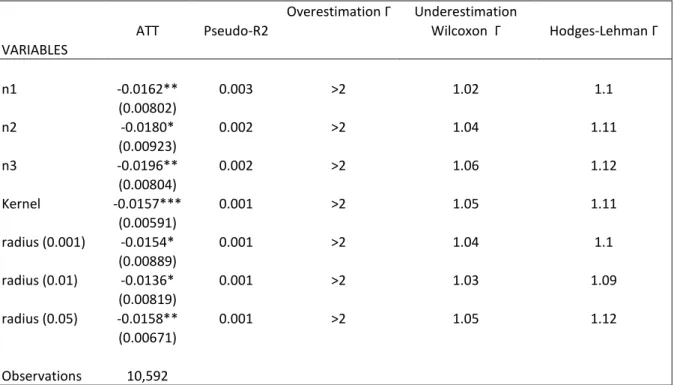
Overestimation Γ Underestimation
ATT Pseudo-R2 Wilcoxon Γ Hodges-Lehman Γ
VARIABLES n1 -0.0162** 0.003 >2 1.02 1.1 (0.00802) n2 -0.0180* 0.002 >2 1.04 1.11 (0.00923) n3 -0.0196** 0.002 >2 1.06 1.12 (0.00804) Kernel -0.0157*** 0.001 >2 1.05 1.11 (0.00591) radius (0.001) -0.0154* 0.001 >2 1.04 1.1 (0.00889) radius (0.01) -0.0136* 0.001 >2 1.03 1.09 (0.00819) radius (0.05) -0.0158** 0.001 >2 1.05 1.12 (0.00671) Observations 10,592
Standard errors in parentheses *** p<0.01, ** p<0.05, * p<0.1
Notes: Rosenbaum bounds are calculated using the command rbounds in Stata. Wilcoxon Γ and Hodges-Lehman Γ are the values above which unobservable information bias our results
Results of the PSM in table 5 show that remittance-receiving households are less poor than non-receiving households. This result is robust to multiple matching techniques, which are the nearest neighbor matching, the kernel matching, as well as the radius matching with different caliper numbers.
Results in table 5 also present the pseudo R2 as well as the rosenbaum bounds, in order to check for the validity of matching assumptions. As we stated earlier, a small pseudo R2 signals that propensity scores can be used as balanced scores. In our case, we see that the pseudo R2 is close to zero, varying between 0.001 and 0.003. These results imply that our matching allows obtaining balanced scores in order to estimate the effect of receiving remittances on poverty.
As we have a continuous outcome variable, we use here rbounds other than mhbounds. Results show that reducing effect of remittances on poverty is highly robust to overestimation of the impact of unobservable on our estimations, as the odds ratio found is greater than 2.
This result is in line with the findings of (Roth,, V and al, 2014) who also find that the reducing effect of remittances on poverty in robust to unobservable variables odds ratio greater than 24.
(Roth, V…) also found that yet for underestimation, the numbers are low, around 1.1. In our case, the level to which our estimations might be questionable varies weather we look at the Wilcoxon results or the Hodges-Lehman point estimates. The results suggest that unobservables characteristics will make our results questionable around an odds ratio between 1.02 and 1.12. These results can be considered sensible to unobserved characteristics when considering the work of Duvendack and Palmer-Jones (2011), who stated that odds ratio below 2 indicate high sensitivity to unobservable. However, this statement can be considered pessimistic (Clement Matthieu & al 2012) as the field of this work cannot be compared to other sciences results such as medicine, where the numbers often exceed 5. Aakvik (2001) also argued that sensitivity analysis describes a
4 We made our calculations for a gamma between (1 (0.01) 2 ) in accordance to the literature. Hence, (Aakvik, 2001)show that an odds ratio of 2 is a very large number. This implies that the estimations will be biased only if unobservables cause the odds to differ between the treated and the non-treated households by 100%.
“worst case scenario” as it portrays how a given treatment effect can alter results and estimations in case of hidden bias, not indicating, then, that such bias do exists.
4.2-Robustness Checks
a- International remittances
Receiving international remittances VS not receiving any remittances
Overestimation Underestimation
ATT Pseudo-R2 Wilcoxon Γ Wilcoxon Γ Hodges-Lehman Γ
VARIABLES n1 -0.0328** 0.005 >2 1.11 1.26 (0.0133) n2 -0.0325** 0.004 >2 1.11 1.23 (0.0133) n3 -0.0329** 0.004 >2 1.1 1.22 (0.0136) Kernel -0.0309*** 0.002 >2 1.1 1.21 (0.00942) radius (0.001) -0.0347*** 0.001 >2 1.12 1.24 (0.0122) radius (0.01) -0.0338*** 0.000 >2 1.12 1.24 (0.00777) radius (0.05) -0.0302*** 0.002 >2 1.09 1.2 (0.0103) Observations 8769
Standard errors in parentheses *** p<0.01, ** p<0.05, * p<0.1
We then chose to check our results by focusing only on international remittances. Therefore, we are trying here to understand if the result is consistent. Table 6 shows that our results are consistent, and the impact is stronger. In fact when comparing the coefficients of the ATT in Table 6 and in Table 5, one can see that they are much higher
for international remittances. Households that receive international remittances seem to be even less poor than those who do not receive remittances.
This result can be explained by the fact that international remittances amounts are higher than internal remittances, despite the fact that households mostly receive the latter. This leads us to comparing households based on the origin of remittances that they receive.
b- International remittances vs internal remittances
Now we try to test the results when comparing international remittances and internal remittances. Households that receive international remittances will be attributed 1 and 0 when they receive internal remittances. Results in table 7 show here that receiving remittances from abroad reduce poverty even deeper than when receiving internal remittances.
Overestimation Underestimation
ATT Pseudo-R2 95% 95% Hodges-Lehman Γ
VARIABLES n1 -0.0430*** 0.001 >2 1.29 1.23 (0.0128) n2 -0.0300*** 0.000 >2 1.17 1.11 (0.0105) n3 -0.0309*** 0.000 >2 1.19 1.13 (0.0108) Kernel -0.0232** 0.000 >2 1.1 1.05 (0.00984) radius (0.001) -0.0292*** 0.000 >2 1.16 1.1 (0.0111) radius (0.01) -0.0261** 0.000 >2 1.13 1.08 (0.0103) radius (0.05) -0.0228** 0.000 >2 1.1 1.04 (0.0100) Observations 2851
Standard errors in parentheses *** p<0.01, ** p<0.05, * p<0.1
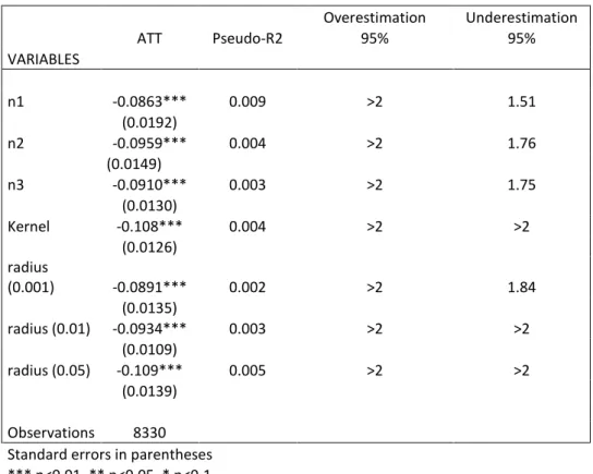
c- 25% Most receiving households. Overestimation Underestimation ATT Pseudo-R2 95% 95% VARIABLES n1 -0.0863*** 0.009 >2 1.51 (0.0192) n2 -0.0959*** 0.004 >2 1.76 (0.0149) n3 -0.0910*** 0.003 >2 1.75 (0.0130) Kernel -0.108*** 0.004 >2 >2 (0.0126) radius (0.001) -0.0891*** 0.002 >2 1.84 (0.0135) radius (0.01) -0.0934*** 0.003 >2 >2 (0.0109) radius (0.05) -0.109*** 0.005 >2 >2 (0.0139) Observations 8330
Standard errors in parentheses *** p<0.01, ** p<0.05, * p<0.1
Targeting households that receive the largest amounts of remittances, we found with table 8 that the results still robust, even if the coefficient of the ATT slightly changes. Compared to the baseline results, the impact of remittances on poverty is higher for this subpopulation.
This result shows that when comparing the most receiving households, to those who do not receive remittances, the former population is much less poor than the latter.
This result can be explained by the fact that households who receive remittances can be those who where able to send a member abroad, and usually are the richest ones. Therefore, when receiving remittances, their living standards will inevitably grow faster.
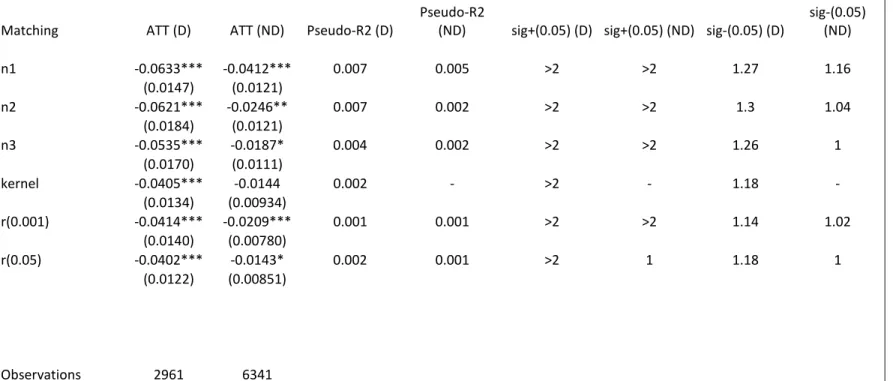
3.3- Remittances and previous disasters
Another interpretation of the computed index lies in the preparedness of households in case of disasters. The work of (Mohapatra & Ratha, D, 2009), found that household in Burkina Faso, that receive remittances tend to live in concrete houses, making them more resilient to disasters. Our index can be seen as a extension of this idea, as it captures some aspects of ex ante dispositions to face natural disasters, such as living in a concrete roof, concrete walls, owning a mobile phone, having a drainage system, and living in a parcelled area, factors that contribute to considerably reduce the probability of experiencing floods, or be more resilient in case of natural disaster.
In this part, we use data from the CONASUR (Conseil National de Secours d’Urgence et de Réhabilitation) of Burkina Faso, which is in charge of rescuing population in case of all nature emergencies and disasters. This database gives the number of disasters that occurred in the country since 2007. We focused on the data of 2013 and 2012, and generate a variable that take the value 1 if the household have experienced floods or violent wind, and zero otherwise5.
5 A simple correlation test shows that the poverty index and the disaster variable are not significantly
Matching ATT (D) ATT (ND) Pseudo-R2 (D)
Pseudo-R2
(ND) sig+(0.05) (D) sig+(0.05) (ND) sig-(0.05) (D)
sig-(0.05) (ND) n1 -0.0633*** -0.0412*** 0.007 0.005 >2 >2 1.27 1.16 (0.0147) (0.0121) n2 -0.0621*** -0.0246** 0.007 0.002 >2 >2 1.3 1.04 (0.0184) (0.0121) n3 -0.0535*** -0.0187* 0.004 0.002 >2 >2 1.26 1 (0.0170) (0.0111) kernel -0.0405*** -0.0144 0.002 - >2 - 1.18 - (0.0134) (0.00934) r(0.001) -0.0414*** -0.0209*** 0.001 0.001 >2 >2 1.14 1.02 (0.0140) (0.00780) r(0.05) -0.0402*** -0.0143* 0.002 0.001 >2 1 1.18 1 (0.0122) (0.00851) Observations 2961 6341
(D) Stands for households who experienced floods and violent wind (ND) Stands for households who did not experience floods and violent wind
We saw in previous results that remittance-receiving households are less poor and more prepared to potential disasters. Results in table 9 now show that households that receive remittances and have previously experienced natural disasters are even less poor than households that did not experienced disasters in the past.
Results in table 9 show that for households that have experienced disasters in the past, remittances acts in a more efficient way. Hence, receiving remittances is lowering more the poverty scores for these types of households, than for those that have not experienced disasters in the past.
Another interpretation is that households, who experienced floods and violent wind, use remittances in a most efficient way when it comes to housing.
Therefore, remittances and past disasters can be seen as important factors in the resilience aspects of Burkina Faso’s households to potential future disasters. However it is difficult to state between an ex ante preparation of households6, or an ex post
reaction.
Conclusion
Migration and climate issues constitue some of the trending topics in international discussions today as they play an important role in the development of countries, especially most vulnerable ones such as those in sub-saharan Africa.
We contribute to the existing debate by investigating the impact of remittances on poverty in Burkina Faso.
The paper is based on a multi-topic household panel survey conducted in Burkina Faso by the “Institut National de la Statistique et de la Démographie” (INSD), in 2014. An index of poverty, taking into account variables that reflect household’s deprivation in housing commodities, helped us to understand the linkages between remittances and poverty. An alternative interpretation of this index allows us to understand the impact of remittances on household’s preparedness to natural disasters.
We used propensity score matching techniques to compare households’ poverty levels when they receive or do not receive remittances.
Our findings go along with the ones in the literature, concluding that remittances reduce poverty. The results are consistent when using different matching techniques, and subsampling.
Using data on the occurrence of floods and violent wind in the country for 2013 and 2012, we found those households that receive remittances, and have been hit by such disaster tend to be less poor, and more resilient.
An important conclusion stems from this result, as we can say that there is a learning process of households when it comes to natural disasters, and that remittances can be an instrument of preparedness for households by making resources available for investments in houses improvements, in order to increase their resilience to disasters (Mohapatra & Ratha, D, 2009).
Rather than seeing remittances as any other income, they should be seen as a contribution that can help reinforcing the efforts made by governments and organizations regarding household’s resilience to natural disasters.
Bibliographie
Acosta, P., Calderon, C., Fajnzylber, P., & Lopez, H. (2008b). What is the impact of international remittances and poverty and inequality in Latin America? World Development , 36, 89-114.
Acosta, P., Calderon, P, Fajnzylber, P, & Lopez, H. (2006). Remittances and development in Latin America . World Economy , 29 (7), 957-987.
Adams, R. H., & Alfredo, C. (2013). The impact of remittances on Investment and poverty in Ghana. World Development , 50, 24-40.
Adams, R., & Page, J. (2005). Do international migration and remittances reduce poverty in developing countries? World Development , 33 (10), 1645-1669.
Adams, R., & Page, J. (2005). Do international migration and remittances reduce poverty in developing countries? . World Development , 33, 1645-1669.
Alkire, K., & Santos, M.E. (2010, July). Acute multidimentional poverty: A new index for developing countries. (O. P. Initiative, Éd.) Human Development Research Paper .
Alkire, S., & Santos, ME. (2010). Multidimentional Poverty Index. Oxford Poverty and Human Development Initiative.
Bambio, Y. (2014). Impact of remittances on poverty and inequality in rural Burkina Faso . Revue d'économie théorique et appliquée , 4 (2), 121-144.
Bardhan,P, & Udry,C. (1999). Development Microeconomics. Oxford Univerty Press. Benzécri, J. (1979). Sur le calcul des taux d'inertie dans l'analyse d'un questionnaire . Cahier de l'analyse de données , 4, 377-378.
Briand, Anne, & Loyal Laré, Amandine. (2013). La demande de raccordement des ménages auprès des petits opérateurs privés d'eau potable: le cas des quartiers de Maputo . Presses de Sciences Po , 64, 685-719.
Caliendo, M, & Kopenig, S. (2008). Some practical guidance for implemation of propensity score matching. Journal of Economic surveys , 22 (1), 31-72.
Craciun, C. (2006). Migration and Remittances in the Republic of Moldova: Empirical Evidence at Micro Level. . National University "Kyiv-Mohyla Academy".
Deaton, A., & Muellbauer, J. (1980). Economics and consumer behavior . Cambridge University Press.
Dehejia, R, & Wahba, S. (2002). Propensity score matching methods for nin experimental causal studies . Review of Economics and Statistics , 84, 151-161.
Durand, J., Kandel, W , Massey, D. S. , & Parrado, E. A. . (1996). International migration and development in Mexican communities. Demography , 33 (2), 249-264.
FAO. (2012). Resilience Index: Measurement and Analysis model .
Filmer, D, & Pritchett, L.H. Estimating Wealth Effects without Expenditure Data or Tears: An Application to Educational Enrolments in States of India. Demography , 38 (1), 115-132.
George Owusu;, & Francis Mensah. (2013). Non monetary poverty in Ghana . Ghana statistical Service .
Greenace, M. (1993). Correspondace Analysis in practice. London: Academic Press . Gubert, S., Mesplés-Somps, S, & Lassourd, T. (2010, Juillet ). Do remittances affect poverty and inequality: evidence from Mali. Document de travail UMR DIAL .
Gupta, S., Pattillo, C.A., & Wagh, S. (2009). Effect of remittances on poverty and financial development in Sub-Saharan Africa. World Development , 37, 104-115.
Hangnon, H., De Longueville, F, & Ozer, P. (2015). Précipitations extrêmes et inondations à Ouagadougou: Quand le développement urbain est mal maîtrisé. XXVIII Colloque de l'association internationale de climatologie , Liège.
Hartwell, M. (1972). Consequences of the industrial revolution in England for the poor. IEA .
Heckman, J, Ichimura, H, & Todd, P. (1998). Matching as an econometric evaluation estimator . Review of Economic studies , 65 , 261-294.
Hervé, A., & Valentin, D. (2007). Multiple correspondance analysis. Encyclopedia of measurement and statistics , 651-657.
Holst, E., & Schrooten, M. (2006). Migration and money- What determines remittances? Evidence from Germany. Institute of Economic Research, Hitotsubashi University,
Discussion Paper Series , 477.
Imai, K., king, G, & Stuart, E.A. (2008). Misunderstandings between experimentalistsand observationalists about causal inference . Journal of the royal statistical society: Series A (Statistics in Society) , 171, 481-502.
Institut National de la Statistique et de la Demographie (INSD). (2015). Rapport Enquête Multisectiorielle Continue (EMC), Phase 1, Rapport Thématique 1, Caractéristiques
Sociodemographiques de la Population . INSD , Ouagadougou . IPC, I. P. (2006). Poverty in Focus. UNDP.
Lachaud, J. (1999). Envois de fonds, inégalités et pauvreté au Burkina Faso. Revue Tiers Monde , 40 (160), 793-827.
Lavell, A. M.-W. (2012). Climate change: new dimensions in disaster risk, exposure, vulnerability, and resilience. In: Managing the Risks of Extreme Events and Disasters to Advance Climate Change Adaptation . A Special Report of Working Groups I and II of the Intergovernmental Panel on Climate Change (IPCC), Cambridge University Press. Le De, L., Gaillard, J. C., & Friesen, W. (2015). Do remittances reproduce vulnerability . Journal of Development Studies , 51 (5), 538-553.
Lee, W. (2013). Propensity score matching and variations on the balancing test. Empirical Economics , 44, 47-80.
Lipton, M, & Ravallion, M. (1993). Poverty and Policy. Policy Research, Poverty and Human Resources .
Lokshin, M., & Bontch-Osmolovski, M. (2010). Work-related migration and poverty reduction in Nepal . Review of Development Economics , 14 (2), 323-332.
Lopez-Cordova, E. (2005). Globalization, migration and development: The role of Mexican migrant remittances . Economia , 6 (1), 217-256.
Mantel, N, & Haenszel, W. (1959). Statistical aspects of the analysis od data from retrospective studies . Journal of the national cancer institute , 22, 719-748.
Mohapatra, S., & Ratha, D. (2009). Remittances and Natural Disasters: ex-post response and contribution to ex ante preparedness. Policy research Working Paper Series , 4972. Moises, S., & Kim Donghun. (2011). How do international remittances affect poverty in developing countries? A quantile regression analysis . Journal of Economic Development , 36 (4).
Randazzo, T., & Piracha, M. (2014). Remittances and Household Expenditure Behaviour in Senegal . IZA Discussion paper , 8106.
Ravallion, M. (1994). Poverty Comparisons, Fundamentals of pure and applied economics (Vol. 56). Harwood Academic Press.
Richard, H. (2006). Remittances and poverty in Ghana . Development Research Group . Rosenbaum, P. (2010). Design of obervational studies . Springer-Verlag .
Rosenbaum, P.R, & Rubin, D.B. The central role of propensity score in observational studies for causal effects . Biométrika , 70 (1), 41-55.
Sen, A. (1987). The Standard of Living. Cambridge University Press , 46.
Sianesi, B. (2004). An evaluation of the swedish system of active labor market programs in the 1990's . Reviews of Economics and Statistics , 86 (1), 133-155.
Sighomnou D., T. B. (2012). Crue exceptionnelle et inondations au cours des mois d'août et septembre 2012 dans le Niger Moyen et Inférieur. Hydrosciences.
Streeten, P, Shahid, JB, ul Haq, M, Hicks, N, & Stewart, F. (1981). First things first: meeting basic needs in developing countries. Oxford University Press .
Vallée, J., Fournet, F, Meyer, PE, Harang, M, Pirot, F, & Salem, G. (2006). Stratification de la ville de Ouagadougou (Burkina Faso) à partir d'une image panchromatique Spot 5: Une première étape à la mise en place d'une enquête de santé. Espace urbain et santé , 2 (3).
World-Bank. (s.d.). The World Bank. Consulté le 2016, sur The World Bank:
http://www.worldbank.org/en/news/press-release/2016/04/13/remittances-to-developing-countries-edge-up-slightly-in-2015
Yang, D., & Choi, H. (2007). Are remittances insurance? Evidence from rainfall shocks in the philippines. The World Bank Economic Review , 21 (2), 219-248.
Appendix
Variable Total
Survey Remittances Internal Receiving HH International Remittances Receiving HH Nb of
HH Unit Data Source
HH Gender 86,27% 74,60% 78,77% 10806 Household Head is a man Enquête Multisectorielle continue (2014)
HH Educate 27% 31,98% 21,56 % 10809 Household Head Educate Enquête Multisectorielle continue (2014)
HH Work 81,09% 70,75% 71,62% 10809 Household Head Working Enquête Multisectorielle continue (2014)
Urban 39,43% 45,55% 30,91% 10852 Household living in an urban
area Enquête Multisectorielle continue (2014)
HH Size 7,27 6,42 7,90 10849 Household’s size Enquête Multisectorielle
continue (2014)
HH Head Age 46 48 51 10806 Household’s Head Age Enquête Multisectorielle
continue (2014) Distance to civil
service 3,49 3,22 3,65 10796 Distance between the household and the registry office measured in minutes
Enquête Multisectorielle continue (2014)
Distance to
practicable road 2,26 2,03 2,37 10798 Distance between the household and the nearest practicable road measured in minutes
Enquête Multisectorielle continue (2014)
Remittances 26.92% 17.92% 8.38% 10852 Remittances receiving HH Enquête Multisectorielle continue (2014)
Disasters 31.39% 29.82% 27.39% 10859 Household’s hit by floods or violent wind during the past months
Conseil National de Secours d’Urgence et de
Appendix 2: Descriptive Analysis
Promiscuity persons live in the same
room continue (2014)
Total per capita
expenditures 272974.5 286379.4 250430.1 10412 Total expenditures divided by the household size Enquête Multisectorielle continue (2014) Luminosity 16.44858 18.99319 14.14309 10667 Nighttime luminosity
intensity
National Center for
Appendix 3: Multiple Correspondence Analysis variable loadings.
These graphs have been obtained with the software TANAGRA. The graph here shows another interpretation of the index, via an index of wealth, rather than poverty. The figures are the same, but this presents another way of seeing the index.
Appendix 4: The Benzecri correction
The Benzecri correction equals to: Tμi = (p/1-p) (μi- 1/p)
MCA_1_Axis_1 vs MCA_1_Axis_2
Concrete Roof Concrete Floor Drainage System Improved Toilet Concrete Walls Mobile Phone Parcelled Area
MCA_1_Axis_1 1 0 M C A_ 1_ Ax is _2 2 1 0 Concrete Roof=No Concrete Roof=Yes Concrete Floor=No Concrete Floor=Yes Drainage System=No Drainage System=Yes Improved Toilet=No Improved Toilet=Yes Concrete Walls=No Concrete Walls=Yes Mobile Phone=No Mobile Phone=Yes Parcelled Area=No Parcelled Area=Yes
Where p represents the number of active variables7, and μi is the ni eigen value. This
calculation is made only for the Eigen values greater that 1/p.
Appendix 5 : Impact of internal remittances on poverty
Overstimation Underestimation
ATT Pseudo-R2 Wilcoxon Γ Wilcoxon Γ
Hodges-Lehman Γ VARIABLES n1 -0.0281** 0.001 >2 1.07 1.16 (0.0125) n2 -0.0182 1 1 (0.0118) n3 -0.0218** 0.001 >2 1.05 1.13 (0.00905) Kernel -0.0150** 0.001 >2 1.01 1.09 (0.00756) radius (0.001) -0.0129 (0.0110) radius (0.01) -0.0147* 0.001 >2 1.02 1.09 (0.00877) radius (0.05) -0.0148 (0.00905) Observations 8627
Standard errors in parentheses *** p<0.01, ** p<0.05, * p<0.1
Notes: Rosenbaum bounds are calculated using the command rbounds in Stata.
7 Variables used to construct the index
Original Values Benzecri correction
Axis Eigen Value
Percentage explained
Histogram Eigen Value Percentage explained 1 0.3052 30.53% 0.035911 93.66% 2 0.1851 18.51% 0,002433 6.34% 3 0.1354 13.55% 4 0.1157 11.58% 5 0.1064 10.65% 6 0.0613 9.05%