HAL Id: hal-01832674
https://hal.archives-ouvertes.fr/hal-01832674v2
Submitted on 18 Feb 2019
HAL is a multi-disciplinary open access archive for the deposit and dissemination of sci-entific research documents, whether they are pub-lished or not. The documents may come from teaching and research institutions in France or abroad, or from public or private research centers.
L’archive ouverte pluridisciplinaire HAL, est destinée au dépôt et à la diffusion de documents scientifiques de niveau recherche, publiés ou non, émanant des établissements d’enseignement et de recherche français ou étrangers, des laboratoires publics ou privés.
Regular Switching Components
Yan Gérard
To cite this version:
Yan Gérard. Regular Switching Components. Theoretical Computer Science, Elsevier, 2019, Special issue of TCS devoted to the memory of Maurice Nivat, �10.1016/j.tcs.2019.01.010�. �hal-01832674v2�
Regular Switching Components
Yan G´erard
LIMOS, University Clermont Auvergne, France
Abstract
We consider a problem of Discrete Tomography which consists of reconstruct-ing a finite lattice set S ⊂ Z2 from given horizontal and vertical X-rays (i.e. with prescribed numbers of points in each row and column). Without addi-tional requirements, the problem can be solved in polynomial time. Many variants require the solution to be in a chosen class A. For instance, the problem is NP-complete for the class A = H ∩ V of HV-convex lattice sets and it is polynomial for the class A = H ∩ V ∩ P of HV-convex polyominoes. Twenty years after these results, the problem’s complexity remains unknown for A = C, the class of C-convex lattice sets (i.e. two-dimensional lattice polytopes).
The main difficulty to solve this problem comes from combinatorial struc-tures called switching components. Switching components are closed path with horizontal and vertical edges such that the solutions S are composed of either the elements of even or of odd indices. This binary choice can be encoded by a Boolean variable associated with the switching component and the convexity constraints are simply encoded by SAT clauses (2-clauses for HV-convexity and 3-clauses for C-convexity).
The purpose of the paper is to investigate the properties of the switching components and the consequences of the convexity requirements. We di-vide the switching components in two classes: regular if their turning angle is constant, irregular otherwise. We prove that adjacent regular switching components have the same Boolean values. This property allows us to merge them into extended switching components. We prove that if all switching components are regular, then the extended switching components are all
in-IThis work has been sponsored by the French government research program
”Investisse-ments d’Avenir” through the IDEX-ISITE initiative 16-IDEX-0001 (CAP 20-25) Email address: [email protected] (Yan G´erard)
dependent (then the number of solutions with the considered feet is 2n, where
n is the number of extended switching components). Finally, we prove that they are geometrically ordered.
Keywords: Discrete Tomography, X-rays, HV-convex lattice sets
1. Introduction
A word about some friends of Maurice Nivat
The scientific community involved in the field of Discrete Tomography started their work about 25 years ago. Maurice Nivat promoted the field by co-organizing or participating in some weeks of workshops in Dagstuhl (1997), Thionville (1999), Sienna (2000), and Oberwolfach (2000). There, he presented the field to younger researchers who became his students and friends. This tribute to Maurice Nivat is also an opportunity to honor the memory of three of his friends who unfortunately died much too early: Alain Daurat, the last PhD student of Maurice (1973-2011), Alberto Del Lungo (1965-2003) [1], and Attila Kuba (1953-2006).
1.1. Open problems in Discrete Tomography
The field of Discrete Tomography [2, 3, 4] started in the mid 90s when the classical algorithms of Computerized Tomography failed to reconstruct lattice sets as requested for instance in Electron Microscopy for the inves-tigation of crystals [5, 6]. Due to the devices providing the measurements and the complexity of the considered problems, special attention has been given to dimension 2. The state of the art around this question was already rich in complexity results, the most fundamental due to D. Gale and R.J Ryser in 1957 [7, 8]. They proved independently that a finite lattice set with prescribed number of points in each row and column can be computed in polynomial time. This central problem has been extended in several direc-tions including the following:
• Increasing the dimension of the lattice: The problem becomes NP-hard from dimension 3 [9]. The question can also be related to timetables and multi-commodity flow problems [10, 11].
• Increasing the number of X-ray directions: An X-ray is the vector which counts the number of points of a lattice set in the sequence of
consecutive parallel lines of given direction. If 3 or more directions are used, then the problem becomes NP-hard [12].
• Reconstructing several disjoint sets: The problem is NP-hard when the objective is to reconstruct two or more disjoint sets from the X-rays [13, 14].
• Adding geometrical or topological constraints as we are going to precise next.
Instead of searching for any lattice set with the prescribed X-rays as in the initial problem investigated by D. Gale and H.G Ryser [7, 8], we can search for a solution satisfying additional constraints. The constraints which are added can be topological, for instance by searching for 4-connected solutions (4-connected finite subsets of Z2 are called polyominoes), or geometrical, as in convex solutions. We introduce for that purpose different classes of lattice sets. The class of the 4-connected lattice sets or in other words polyominoes is denoted P. The lattice sets having consecutive points on each horizontal line are horizontally convex or equivalently H-convex. Their class is denoted H. In the same way, V is the class of the vertically convex namely V-convex lattice sets. By intersection, H ∩ V is the class of the HV-convex lattice sets (Fig. 1). We end these notations with the class C of the C-convex lattice sets in the usual meaning of convexity. A lattice set is C-convex if it is equal to the intersection of its real convex hull with the lattice (Fig. 2). In other words C is the class of the lattice polytopes. Both C-convex and HV-convex lattice sets are not necessarily 4 or even 8-connected. The class of the HV-convex polyominoes i.e 4-connected HV-convex lattice sets is denoted H ∩ V ∩ P.
The reconstruction of lattice sets with prescribed X-rays and belonging to a chosen class has been started by two seminal papers:
• The first one is due to Richard Gardner and Peter Gritzmann[15]. They considered the reconstruction of C-convex lattice sets with different number of directions of X-rays. They characterized the sets of n direc-tions for which any C-convex set is uniquely determined by its X-rays. For 2 or 3 directions, there always exist ambiguous pairs or triplets of X-rays. For n ≥ 7 directions, all C-convex lattice sets are uniquely determined by their X-rays. For 3 < n < 7, the so-called cross-ratios of the directions provide a characterization of the sets of directions with either the uniqueness property, or ambiguous X-rays [15]. When the
Figure 1: HV-convexity. The two left lattice sets are not HV-convex since their in-tersection with some vertical or horizontal line has holes. The two right lattice sets are HV-convex.
Figure 2: C-convexity. The left lattice set is not C-convex since its convex hull contains a lattice exterior point (in white). The right lattice set is C-convex.
directions of X-rays provide uniqueness, these results have been com-pleted by a polynomial time reconstruction algorithm by Sara Brunetti and Alain Daurat [16].
• The second paper on which we focus our attention is the reconstruction of HV-convex polyominoes of Z2 from their horizontal and vertical X-rays. Elena Barcucci, Alberto Del Lungo, Renzo Pinzani, and Maurice Nivat proved in 1996 that this problem can be solved in polynomial time [17].
The polynomial time algorithm reconstructing a solution in the class H ∩ V ∩ P from their horizontal and vertical X-rays is all the more noteworthy that almost all other related problems are NP-hard. Deciding whether there
exists a solution in the classes H, V, H ∩ V, P (or more generally with neighborhood constraints) is NP-complete in these cases [18, 17, 19]. The main remaining open question with orthogonal X-rays is the complexity of the reconstruction of lattice polytopes or in other words C-convex lattice sets [20]. It is a challenging problem whose adjacency with the reconstruction of HV-convex polyominoes has drawn a new attention on the original algorithm of [17]. Experts have noticed for twenty years that the 2-CNF formula built at the last step of the algorithm is always satisfiable (oral communications). However, this proposition remains a conjecture. Maurice Nivat and his co-authors left part of the combinatorial structure of the problem unsolved, although these questions are of major interest to tackle the remaining open problems of Discrete Tomography.
1.2. Results
In this paper, we provide new results in the framework of the reconstruc-tion of lattice sets from their horizontal and vertical X-rays with convexity constraints. The reconstruction can be done by a generic algorithm denoted ConvexTomo whose strategy has been first described in [17] and also used in [21, 16]. ConvexTomo computes a partial solution and expresses the ambigu-ities about the remaining part in combinatorial structures called switching components. These structures are closed path with vertices on the lattice and only horizontal and vertical edges. Any switching component P provides two different ways to complete the partial solution, either by adding the vertices with odd indices or the ones with even indices. This binary choice is en-coded by a Boolean variable denotes P (S), where the argument S ⊂ Z2 is
the considered lattice set.
We divide the switching components in two classes according to the vari-ation of their turning angle: They might turn sometimes to the left (counter-clockwise) and sometimes to the right ((counter-clockwise). If the path always turns to the same direction, the switching component is regular, and irregular oth-erwise. A larger part of the paper is devoted to the regular case.
The main lemma of this work (Lemma 1) is that adjacent regular switch-ing components are equivalent in the sense that the convexity constraints enforce their Boolean variables to be equal. It follows that in the case where all the switching components are regular, any pair of switching component is either equivalent or independent (Theorem 1). This property allows us to merge the equivalent switching components into extended switching compo-nents. These objects are all independent. It provides the following structural
property:
Given a chosen position of the feet (the points of a solution with extremal coordinates), if the switching components can be computed and if they are all regular, then the number of solutions (with the chosen feet) is 2n where
n is the number of extended switching components (Property 1).
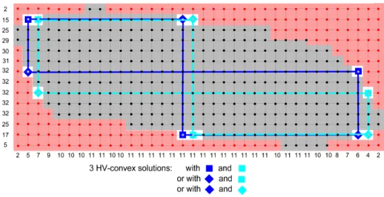
This property does not hold in general: with irregular switching compo-nents, the number of solutions is not necessarily a power of 2 (an example with 3 solutions is presented in Fig.3).
As the condition of regularity of all the switching components may seem a bit restrictive, we investigate the different cases in which it might occur. It leads us to prove new properties of the switching components and to provide some non-intuitive counter-examples.
• We prove that each switching component visits necessarily the four areas (South West, North West, North East and South East) of the set of undetermined points (Property 2).
• Except in one configuration of the feet (configuration e) of Figs. 20 and 21), the switching components are either all regular, or all irregular. In configuration e), we might have both regular and irregular switching components (this counter-intuitive case is illustrated in Fig.23). • We prove that if all switching components are regular, then the
ex-tended switching components obtained by merging the adjacent switch-ing components are well ordered (Property 3).
These properties might be helpful to reconstruct in polynomial time C-convex lattice sets from their horizontal and vertical X-rays at least in the case of regular switching components [22].
In Section 2, we state the problem DTA, present the classical approach
ConvexTomo and introduce the switching components. In Section 3, we prove the main result about the equivalence of the adjacent regular switching com-ponents. At last, Section 4 is devoted to the additional results (Properties 2 and 3).
2. Problem statement and generic algorithm ConvexTomo
First we introduce the notion of X-rays in order to state the problem DTA. Secondly, we present the classical generic algorithm ConvexTomo. This
Figure 3: Counter-example with irregular switching components. Given pre-scribed X-rays h = (5, 17, 25, ...) and v = (2, 5, 7, 9, ...), we are searching for an HV-convex or C-convex lattice set with the prescribed X-rays. A partial solution can be computed. Some lattice points are inside the solution (black points, green cells), some lattice points are excluded (red points, pink cells) while some points remain undetermined (grey points,white cells covered by blue and cyan diamonds and squares). The blue path joining alternatively the blue squares and diamonds by horizontal and vertical edges is a switching component, and the same for the cyan path. These two switching components are both irregular since their path turn sometimes clockwise and sometimes counterclockwise. With these switching components, we can complete the partial solution by adding either the blue squares or the blue diamonds and either the cyan squares or the cyan diamonds (but not both). These two binary choices are encoded by two Boolean variables. The constraints of convexity make them dependant. If we add the blue squares, then we have to add cyan squares (if we add the cyan diamonds, then we have to add the blue diamonds). Due to this relation, we have here exactly 3 solutions. We prove in the following that with regular switching components, the number of solutions is necessarily a power of 2 (Property 1). This example shows that there is no hope to extend this property to the irregular case.
algorithm requires the class A to be included in H ∩ V and to satisfy the partition property described later. These two assumptions allow us to define switching components.
2.1. Horizontal and vertical X-rays
An X-ray is the sequence of the cardinalities of the intersection between a given lattice set and the consecutive diophantine lines in a given direction.
In the case of the vertical and horizontal directions, it leads to the following definition.
Definition 1. Given a finite lattice set S ⊂ Z2 included in the rectangle
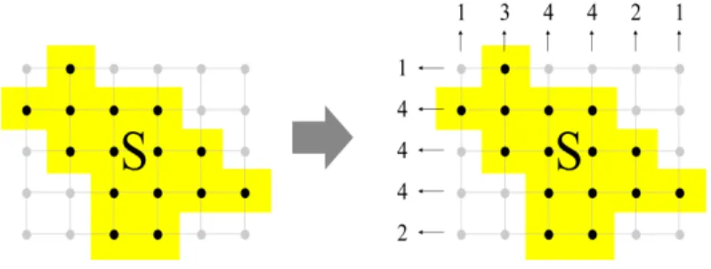
[1, m] × [1, n], its vertical X-ray is the vector V (S) ⊂ Zm whose coordinate vi(S) is the number of points of S in the vertical line x = i (we have Vi(S) =
|{(x, y) ∈ S|x = i}|). The horizontal X-ray of S is the vector H(S) ⊂ Zn
counting the number of points of S in each horizontal line y = j (we have Hj(S) = |{(x, y) ∈ S|y = j}|) (Fig. 4).
Figure 4: The horizontal and vertical X-rays of a given lattice set S.
2.2. Problem statement
We introduce the problem of deciding whether there exists a finite lattice set in a given class A with prescribed X-rays:
Problem 1 (DTA(h, v)).
Given a class A of lattice sets
Input: Two vectors v ∈ Zm, h ∈ Zn
Output: Does there exist a lattice set S ∈ C with V (S) = v and H(S) = h? The problems DTA are known to be polynomial for the classes A of the
whole lattice sets [7, 8] and for the class H∩V ∩P of the HV-convex polyomi-noes [17]. Its complexity is unknown for the class C of the C-convex polytopes and is NP-complete for many other classes (H, V, H ∩ V, P or lattice sets with neighborhood relations) [18, 17, 20].
2.3. The feet
We define the feet of a lattice set S as the subsets of its points with minimal or maximal coordinates.
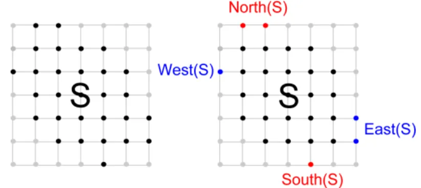
Definition 2. Given a finite lattice set S ⊂ Z2, we consider its South, East, North and West feet as the sets
• South(S) = S ∩ {y = ymin(S)} where ymin(S) is the min ordinate of
the points of S.
• West(S) = S ∩ {x = xmin(S)} where xmin(S) is the min abscissa of the
points of S.
• North(S) = S ∩ {y = ymax(S)} where ymax(S) is the max ordinate of
the points of S.
• East(S) = S ∩ {x = xmax(S)} where xmax(S) is the max abscissa of the
points of S.
Figure 5: The feet. The four feet of a finite lattice set.
2.4. Generic algorithm ConvexTomo
The original algorithm of [17] has been developed for the reconstruction of HV-convex polyominoes (DTH∩V∩P), but it can be applied to solve DTA
with other classes A than H ∩ V ∩ P. It requires two assumptions on A. The first one is that the class A is included in the class H ∩ V of the HV-convex lattice sets. The second requirement is less direct. We present it after the introduction of the filling operations.
The generic algorithm ConvexTomo issued from [17] and used to solve DTA
can be decomposed in four steps: 1. Fix the feet (Fig.6).
2. Perform the filling operations: Take the X-rays and the geometrical constraints into account in order to compute a partial solution. Pro-ceed until the filling operations do not allow to add or exclude any undetermined point.
3. If it remains undetermined points, connect them in path called switch-ing components and represent the binary choice of addswitch-ing either the points with odd or even indices by a Boolean variable.
4. Express the condition that the lattice set S is in the given class A by SAT clauses and solve the SAT instance.
Figure 6: Step 1. On the left, the different possible positions of the feet. On the right, a position of the feet is chosen. The points are added in In (this set is represented by the black points/grey cells) while the other extreme points which have not been chosen are added in Out (red points/pink cells). The shell (grey points/white cells) is the set of the points which are not yet determined.
2.5. Filling operations
Given the chosen feet, the filling operations used for solving DTA work
• The set In contains the points which are known to belong to all solu-tions.
• The set Out contains the points which are known to be excluded from all solutions.
• The set Shell is the set of the undetermined points.
The task of the filling operations is to take the constraints into account in order to include or exclude as many points as possible and thus decrease the cardinality of the shell (some filling operations are sketched in Fig.7). If a point of In has to be added to Out or conversely, this contradiction leads to the conclusion that the considered position of the feet admits no solution. The next step starts when the filling operations did not find any contradiction and are no longer able to decrease the shell size.
There exist different kinds of filling operations depending on the chosen class A. The property of HV-convexity and the prescribed X-rays provide the main operations. The first operations are uniquely related to HV-convexity. The intermediary lattice points between two points of In on the same row or on the same column can be added to In. If there are two points p ∈ In and p0 ∈ Out on the same row or column, then the points p00 with p0 ∈ [pp”] can
be added to Out. There are also filling operations which take the prescribed X-rays into account with HV-convexity (Fig.7). We refer to [21, 16] for a complete presentation of the operations.
Some of the filling operations can be much more complex. It is the case of the operations based on the 4-connectivity used for reconstructing HV-convex polyominoes [17].
2.6. Second assumption: partition property
The algorithm ConvexTomo works under the assumption that the set of undetermined points can be decomposed in switching components. It requires first to provide a partition of the shell in four subsets that we denote NW, NE, SE, and SW for North-West, North-East, South-East and South-West according to their relative location towards the partial solution In (Fig. 8). We call partition property the property that after the end of the filling oper-ations, the position of the solutions are sufficiently determined to decompose the shell in these four regions NW, NE, SE, and SW. Therefore there are only two assumptions to use the generic algorithm ConvexTomo for DTA:
Figure 7: Four filling operations. Each rectangle presents a configuration of the set In (black points) and of the set Out (the excluded points are in red). Due to HV-convexity, the two upper configurations lead to include or exclude new points. Below, the values of the horizontal X-ray allow again to increase In or Out.
2. The partition property namely the guarantee that the shell provided by the filling operations associated with A can always be partitioned in four parts NW, NE, SE, and SW according to their locations. The classes H ∩ V ∩ P and C both verify these requirements. They are both included in H ∩ V. For H ∩ V ∩ P, the filling operations based on 4-connectivity provide a 4-connected set In [17]. Then, any 4-path joining the four feet provides the partition of the set of the undetermined points. It provides the partition property. In the case of the C-convex lattice sets, the convex hull of the feet in R2 provides directly a partition of the shell in four
areas (Fig. 8).
Then the algorithm ConvexTomo can be applied to solve DTA(h, v) for
A = H ∩ V ∩ P or A = C but in order to remain as general as possible, we just assume in the following that the condition A ⊂ HV and the partition property are satisfied. The reader should keep in mind that the whole paper is devoted to the decision problem DTAwith A satisfying these two assumptions.
2.7. Corresponding points
We define vertical correspondences between the South and the North points and horizontal correspondences between the West and the East points. Definition 3. We consider an instance DTA(h, v) with X-rays h and v and a
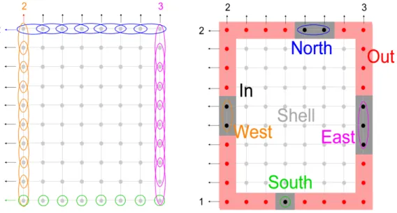
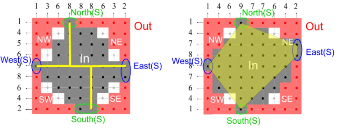
Figure 8: The 4 areas of the shell. On the left, we show an instance of DTH∩V∩P(h, v).
After the filling operations associated with H ∩ V ∩ P, the set In is 4-connected. A 4-path connecting the feet is drawn in yellow. It provides the partition of the grey undetermined points in South-East, North-East, North-West, and South-West areas respectively denoted SE, NE, NW, and SW. On the right, we consider an instance of DTC(h, v). The partition
of the shell in SE, NE, NW, and SW is given directly by the convex hull of the feet.
provide a shell which can be decomposed in four areas SE, NE, NW, and SW.
The vertical correspondent of a point p = (i, j) of the South areas SE∪SW is the point p = (i, j + vj).
The vertical correspondent of a point p = (i, j) of the North areas NE ∪ NW is the point p = (i, j − vj).
The horizontal correspondent of a point |p = (i, j) of the West areas SW ∪ NW is the point p| = (i + hj, j).
The horizontal correspondent of a point p| = (i, j) of the East areas SE ∪ NE is the point |p = (i − hj, j).
The vertical and horizontal correspondents have several properties. 1. The horizontal and vertical correspondents of an undetermined point
p are also undetermined (otherwise, the filling operations allow us to assign p to In or Out).
2. Correspondences are symmetric relations.
3. If p is in a solution, then its correspondents are outside.
4. A point p and its correspondent p0 cannot be both outside a solution because the segment of the solution is necessarily in between and there are not enough points.
Figure 9: Corresponding points. On the left, a configuration with the sets In (black points), Out (red points), and Shell (white cells, grey points) of the undetermined points. In the middle, a pair of vertical correspondents (green) and a pair of horizontal corre-spondents (blue). We represent the points alternatively with squares or diamonds. Notice that the segment represented by the dotted ellipse has only two possible positions. Due to its length, if it contains the square, then it does not contain the diamond and conversely. On the right, the correspondences define closed paths called switching components which provide a partition of the undetermined points. For each switching component, either the squares or the diamonds belong to a solution.
It follows that if p and p0 are correspondents, then p is in a solution S if and only if p0 is not in S.
2.8. Switching components
The correspondences between the points define paths. The undetermined point p1has a horizontal correspondent p2which has a vertical correspondent
p3 which has an horizontal correspondent p4 and so on until we come back to
p1as the vertical correspondent (since the shell is finite, the path is necessarily
closed). This path is referred as a switching component (Figs. 9 and 10). Definition 4. We consider an instance DTA(h, v) with a class A ⊂ H ∩ V
satisfying the partition property. The shell provided by the filling operations is decomposed in SE, NE, NW, and SW.
A switching component P is a closed path of corresponding points prwith
indices r ∈ Z/2lZ (the length of the sequence is 2l) so that p2k and p2k+1 are
vertical correspondents, while p2k−1 and p2k are horizontal correspondents
(Fig. 10). We denote by P [0] the set of the vertices with even indices and by P [1] the set of the vertices with odd indices.
Figure 10: Switching components. On the left, two switching components P1 and
P2. The squares represent their points with even indices (the set P [0]) and the diamonds represent the points with odd indices (the set P [1]). Notice that there are only 2 C-convex solutions since the C-convexity forces adding P1[0] ∪ P2[0] or P1[1] ∪ P2[1] to the solution while the sets including P1[0] ∪ P2[1] or P1[1] ∪ P2[0] also have the prescribed X-rays but are not C-convex. In the middle, regular switching components are not restricted to only one turn (the brown switching component makes 2 turns). On the right, an irregular switching component. It turns clockwise at point 2 and counterclockwise at point 3. On the contrary, the switching components of the two left images are regular (they always turn clockwise).
By construction, the two sets P [0] and P [1] have the same horizontal and vertical X-rays, since each point has a unique vertical and horizontal corre-spondent in the other set (they are respectively represented with diamonds and squares in all figures). In the same way as the corresponding points, any solution S of DTA(h, v) with the considered feet falls in one of the two
possible cases:
• either P [0] ⊂ S and P [1] ∩ S = ∅, • or P [1] ⊂ S and P [0] ∩ S = ∅.
In other words, considering a switching component P , a solution contains either the points of the switching component with odd indices or the ones with even indices.
2.9. Boolean variables for encoding the state of each switching component The two possible states of a switching components P in a solution S are encoded by a Boolean variable denoted P (S). Its value is null if P [0] is in
S and P [1] is excluded while P (S) = 1 if P [1] is in S and P [0] is excluded. If we consider the whole sets of switching components Pq for the indices q going from q = 1 to the number Q of switching components, then the values of the Q Boolean variables Pq(S) provide a complete characterization of S.
Moreover, the 2Qpossible assignments of the Q Boolean variables all provide
a set S with the prescribed horizontal and vertical X-rays. The problem is to determine whether there exists an assignment which provides a solution S in the chosen class A.
2.10. Encoding the convexity with clauses
The search for an assignment of the Boolean variables which provides a solution S in the chosen class A is done by expressing the constraints issued from A on the Boolean variables associated with the switching components. With HV-convexity, E. Barcucci et al. have proved that the HV-convexity constraints can be expressed by a 2-CNF formula i.e a conjunction of SAT clauses with at most 2 literals per clause (Fig.11) [17].
The same approach holds for encoding C-convexity with SAT clauses (Fig.11). The number of literals is however no more bounded by 2. Clauses with 3 literals might be necessary with the difficulty that 3-SAT is no more polynomial but NP-complete. It explains why, as far as we know, ConvexTomo is not polynomial for solving DTC. A better understanding of the relations
between the switching components might be of interest in order to develop an alternative approach.
3. Main result
We prove that the Boolean variables associated with adjacent regular switching components are necessarily equal. Then we consider that the switching components are equivalent. This main proposition allows to state several properties.
3.1. Regular switching components
Before investigating the relationships between the switching components, we divide them in two groups according to the regularity of their turning angle.
Definition 5. A switching component is regular if the turning angle at each vertex has a constant orientation (in other words, the switching component always turns clockwise, or always counterclockwise (Fig.10)).
Figure 11: 2-SAT and 3-SAT clauses encoding convexity. The switching compo-nents being encoded by Boolean variables (represented here geometrically with colored squares and diamonds), HV-convexity is expressed by a conjunction of 2-SAT clauses. Consequently, the search of an HV-convex solution is reduced to a 2-SAT instance that can be solved in linear time [23]. For expressing the C-convexity in the same manner, we need clauses with 3 literals. It leads to the difficulty that 3-SAT is NP-complete.
The switching components which have both clockwise and anticlockwise turning angles are simply said irregular (Fig.10).
3.2. Adjacent switching components
We define an adjacency relation between switching components. Two switching components P and P0 are adjacent if they contain respectively a point p and a point p0 which are 4-adjacent.
3.3. Adjacent regular switching components are equivalent
We provide a first explanation about the property that the 2-CNF formula expressing the HV-convexity of a solution of DTA(h, v) can be often reduced
to a set of equalities.
Lemma 1. We consider an instance of DTA(h, v) with a class A ⊂ H ∩ V
satisfying the partition property (Section 2.6). The four feet being chosen and the filling operations performed, the Boolean variables of any pair of adjacent regular switching components are equal.
This lemma can be understood as follows. If P and P0 are two switching components with an adjacent pair of points p1and p01, then the HV-convexity
constraint provides a first relation of dependency: if p1 is in S, then p01 is in
S. It can be formulated by the 2-clause P (S) ∨ P0(S). According to Lemma 1, at some other places, some other points of the two switching components provide necessarily the converse clause P (S) ∨ P0(S) with the consequence that P (S) and P0(S) are necessarily equal.
Proof. We assume w.l.g that the points p1 = (x1, y1) and p01 = (x 0 1, y
0 1) both
belong to the North West area NW and that p01 is the right 4-neighbor of p1
(Fig.12).
Figure 12: Assumption of Lemma 1. We consider two adjacent switching components. By symmetries, we can assume w.l.g that p01is the right 4-neighbor of p1. It follows by
H-convexity that if p1is in the solution S (the odd part P [1] of the switching component P is
in S namely P (S) = 1), then p01is also in S (the odd part P0[1] of the switching component
P0 is also in S namely P0(S) = 1). The black zone is a sketch of the set In. It underlines the property that with regular switching components horizontal correspondences are only between NW and NE or SW and SE while vertical correspondences are only between NW and SW or NE and SE.
We consider the positions of the points p0 = (x0, y0) (vertical
correspon-dent of p1), p2 and p3 = (x3, y3). We distinguish three cases according to the
comparison of y0 and y3.
• Case 1. y0 < y3
• Case 2. y0 = y3
• Case 3. y0 > y3
Figure 13: The three possible configurations used for proving Lemma 1. We develop the three cases in the following.
The three cases are developed in Figs. 14, 15, and 16. We follow the path of the second switching component P0 by starting from p01. This starting point is in the region denoted A in Figs. 14, 15, and 16. We compute the oriented graph of correspondences between the regions reached by P0. This graph provides a description of all the possible paths and thus of all the possible configurations starting from the region A.
According to the relative position of p01 towards p1, the HV-convexity
implies the clause P (S) ∨ P0(S). Some regions provide the converse relation P (S) ∨ P0(S) which provides the equality P (S) = P0(S). They are colored in grey in all the figures. Therefore the task of the proof is to show that any closed path starting from p01 passes necessarily through a grey region. We prove it by computing the graphs of the correspondences of the regions as drawn in Figs.14 and 15.
In the first and second cases (Figs.14 and 15), either the path passes through a grey region and provides the equality, or it cannot come back to the initial region A which is excluded since the path is closed. It provides the equality.
Figure 14: Case 1. In the first case, we decompose the four areas in different regions and follow the path of the switching component P0. It starts with a point p01 in the region A.
The path ends also necessarily in A. Due to the relative position of p01 towards p1, we
have P (S) = 1 =⇒ P0(S) = 1. The horizontal correspondents of the points in region A are either in region B, or in region C. The graph of the correspondences between the regions that we can reach from region A is drawn below. It the switching component P0 passes through one of the grey regions B or F , the HV-convexity constraint leads to P (S) = 0 =⇒ P0(S) = 0. If it passes through the grey regions E or I, then HV-convexity leads to P0(S) = 1 =⇒ P (S) = 1. Therefore, if the switching component passes through one of the four grey regions, then we have the equality P (S) = P0(S). We notice at last that the only way to avoid the grey regions is to follow the path (CDGH)∗ but it is excluded because it would not be possible to end the path in region A.
Figure 15: Case 2. The second case is similar to the first one. Starting from a point p01
in the region A, the path of the switching component either passes through a grey region which provides the equality P (S) = P0(S) or has a cycle (CDGH)∗ which does not allow
to end the path in region A. This last possibility is excluded.
the regions issued from the position of the points p1, p2, and p3 of P . We
introduce four regions denoted A, B, C and D represented in the first row of Fig.16. Then we consider four points of P0. The two first points p01 and p02 are respectively in A and B. For the two other points, we assume that the switching component P0 has two horizontal correspondents respectively in C and D. The four possible cases with such a configurations are drawn in the second row of Fig. 16. These four points of P0 being fixed, we come back to P and try to continue the path P after p3 in order to close it. The considered
path P passes through one of these regions, then the equality P (S) = P0(S) is guaranteed by HV-convexity. These grey regions that the path P should avoid in order to have P (S) 6= P0(S) are drawn in the third row of Fig. 16. If the switching component P avoids the four grey regions, then the figure 16 shows that the path P after p3 is restricted to a green region which does
not allow to come back to the initial point. This case can be excluded, it leads to the following partial conclusion (i): If the switching component P0 has two horizontal correspondents in the regions C and D, the equality of P and P0 is guaranteed.
Figure 16: Case 3. Preliminary analysis. We introduce four regions A, B, C and D. The point p1 and p2 have coordinates noticed (x1, y1) and (x2, y2). The points p01=
(x1+ 1, y1) and p02= (x2+ 1, y2) (in red) are respectively in A and B. In the second row,
we assume that there is a pair of horizontal correspondents of P0 in the regions C and D. We denote their abscissa u and v with u < v. Four sub-cases are possible: u > x1 and
v = x2+ 1, u = x1and v = x2+ 1, u = x1 and v > x2+ 1, u > x1 and v > x2+ 1. In the
third row, we consider the path of the switching component P after p3 (in blue). Either
it passes through one of the grey regions induced by P0 and which provide the equality between P and P0, or it is maintained in the green area which does not allow to come back to p1. This last case is excluded with the consequence that if P0 has two horizontal
We come back to the path followed by the switching component P0 as drawn in Fig.17. We partition the undetermined points in regions according to their positions relatively to p0, p1, p2 and p3 and investigate again the
regions crossed by the switching component P0. The grey regions drawn in Fig.17 are the ones which, due to HV-convexity, provide the equality of the switching component P (S) = P0(S). The diagram of the correspondences between the regions shows that either P0 passes through a grey region, or passes through the edge BC for which the conclusion (i) provides already the equality P = P0, or is not closed which is in contradiction with its definition. It follows that in all valid cases, we have the equality P (S) = P0(S).
3.4. Extended switching components are independent
We consider the case where all the switching components are regular. Lemma 1 provides the following corollary:
Theorem 1. We consider an instance of DTA(h, v) with a class A ⊂ H ∩ V
satisfying the partition property. The filling operations allow us to compute the switching components (Fig.11). If they are all regular, then any pair of switching components P and P0 is either equivalent (for any solution S, P (S) = P0(S) with the convention the first point of any switching component is in NW) or independent.
Proof. We assume that the HV-convexity constraint provides a dependency between two switching components P and P0. It means that they are in a configuration where if a point pk of P is in a solution S, then the point p0k0 of
P0 is also in S. By symmetries, we assume pk = (xk, yk) is in the North West
area. It follows that p0k0 is its South East quadrant {(x, y) ∈ NW|x ≥ xk, y ≤
yk} (Fig.18). Thus there is a 4-connected path of undetermined points from
pk to p0k0. By induction, Lemma 1 proves that their switching components
are all equivalent and thus, provides the equality P (S) = P0(S).
Theorem 1 states that we have either equivalent or independant switching components It leads to merge the equivalent switching components in one single extended switching components.
Definition 6. We consider an instance of DTA(h, v) with a class A ⊂ H ∩ V
Figure 17: Case 3. Final analysis. We partition the areas in regions according to their relative positions towards the points p0, p1, p2 and p3. Due to HV-convexity, if the
switching component P0 has a point in one of the four grey regions W , X, Y and Z, then we have the equality P (S) = P0(S). The oriented graph of the horizontal and vertical correspondences between regions is drawn below. It characterizes the possible path P0 starting at p01. Either it passes through a grey region, or it passes through the edge CD for which we have already proved the equality (i), or we arrive to (CF GB)∗, the path can not be closed and as previously, this case can be excluded. In the two valid cases, P (S) = P0(S).
An extended switching component eP is the union of all the switching components P0 (considered as the set of their points) whose Boolean variables are equal to P due to HV-convexity (Fig.19).
Any extended switching component eP is a subset of the shell. We denote e
Figure 18: A 4-connected path. HV-convex dependencies between switching compo-nents arise for instance in the case where the point p0k0 of the switching component P0is in
the South East quadrant of pk (in yellow). If pk is in a solution S, then by HV-convexity,
p0k0 is also necessarily in S. In any case, we can connect pk and p0k0 by a 4-connected path
of undetermined points (in brown). As their switching components are assumed to be all regular, according to Lemma 1, all the switching components of these brown points are equivalent. It provides the equivalence between the switching components of the blue and red points.
Figure 19: Extended switching components. On the left, due to HV-convexity, the switching components P1, P2, P3, P4are necessarily equal while P5 is independent. On
the right, we merge P1, P2, P3, P4 in the extended switching component fP1 and P5
becomes fP5. Extended switching components are less structured, they are just sets of
points.
definition, for any solution S of the instance DTA(h, v), either ePNW∪ ePSE is
∅. Theorem 1 means that if all the switching components are regular, all extended switching components are independent. An obvious corollary of Theorem 1 is therefore the following property:
Property 1. We consider an instance of DTA(h, v) with a class A ⊂ H ∩
V satisfying the partition property. Given a position of the feet, if all the switching components are regular, then the number of solutions (with the chosen feet) is 2n where n is the number of extended switching components.
Property 1 does not hold with irregular switching components. A case with 3 solutions is shown in Fig.3. We end this section with a last remark about extended switching components in the regular case. Under the as-sumption that all the switching components are regular, distinct switching components pass necessarily through distinct rows and columns. Otherwise they would have been merged. This property is used for ordering the ex-tended switching components.
4. Complementary results
We come back to the general switching components and provide several properties. We are interested in the characterization of the configurations where all the switching components are regular.
4.1. Any switching component visits the 4 areas
Due to their constant turning angle, the regular switching components have a cyclic property. With an initial point p1 chosen in NW, we have
p1+4k ∈ NW, p2+4k ∈ NE, p3+4k ∈ SE, p4k ∈ SW. This property does
not hold with irregular switching components. We can even ask whether an irregular switching component can avoid one of the four areas NE, NW, SW, SE.
Property 2. Any switching component passes through the four areas NE, NW, SW, SE.
Proof. We assume w.l.g that there exists a switching component P which does not pass through the area NE. We start from a point pk ∈ NW and
follow the path of the switching component. The horizontal correspondent pk+1 of pk is necessarily in SE. The vertical correspondent pk+2 of pk+1 is
therefore in NW. By induction, for any positive integer n, we have pk+2n ∈
N W and pk+2n ∈ SE. The turning angles are alternatively +π2 and −π2. Such
4.2. Structure of the switching components according to the positions of the feet
We investigate the relations between the positions of the feet and the structure of the switching components. In order to determine them, we start with an initial position of the South and North feet, and consider all the possible cases by adding first the West foot and secondly the East foot. This investigation is described step by step in Fig.20.
We can assume without loss of generality that the South foot is on the left of the North foot. We notice that the vertical X-rays passing through the South and North feet determine completely these columns (and we will have the same property with the rows of the East and West feet). Then, two cases are possible: either the points of In determined by the South and North feet have a common row or they don’t share any row. In both cases, we introduce the possible positions of the West foot. The points of In on the rows of this foot might have different configurations. Many of them are not HV-convex. After three feet, it remains only three possible cases. By adding the last East foot, we obtain 8 configurations which can be reduced to 6 by removing the symmetric cases. We denote them with letters from a) to f) (Fig.20). Each of them has specific possible switching components (Fig.21). • In case a), different structures of switching components are possible
but they are necessarily irregular (Fig.22).
• In case b), the structure of the switching components is constrained. They are all irregular (Fig.22). The points pk and pk+8 are in the same
area of the shell. Moreover, starting from an initial point p1 in the
South West area, there is no area containing simultaneously points of switching components with odd and even indices. It follows that the constant assignment P [S] = 0 for all switching components, or the constant assignment P [S] = 1 are two trivial solutions of the instance. In other words, there are at least two solutions.
• In case c), we can have switching components with different structures, but necessarily irregular (Fig.22).
• In case d), the structure of the switching components (all irregular according to Fig.22 ) is constrained. The point pk+6 is in the same area
Figure 20: The possible configurations of the rows and columns of the feet. For the clarity of the figure, the lattice points are represented by the square cell which surrounds them. We start with the position of the South and North feet and consider all the compatible cases with HV-convexity by adding the West and East feet. It leads at the end to only 6 possible configurations denoted with letters from a) to f) (the configurations b) and b’) as well as d) and d’) are symmetric).
two trivial solutions obtained with constant assignments of the Boolean variables.
• The case e) is the unique configuration which admits simultaneously irregular and regular switching components. Such a case is illustrated in Fig.21. This example goes against intuition.
Figure 21: The switching components in the 6 possible configurations. Above the positions of the feet (blue and orange) and below, the six different possible configurations obtained in Fig. 20. The set Out of the cells of the excluded points is colored in red and the region of the possibly undetermined points is in grey. In each configuration, we have different structures of switching components. Regular switching components are only possible in the cases e) and f). Irregular switching components are possible in the cases a), b), c), d) and e).
• In the case f), all the switching components are regular.
It remains a lot of open questions about irregular switching components. The case e) is the only one where irregular and regular switching components might exist together (Fig.23). In the cases b), d), and f), the structures of the switching components guarantee that the two constant assignment of the Boolean variables (P (S) = 1 for all switching components or P (S) = 0 for all switching components) are trivial solution. In the configuration a), c) and e), we still don’t know if it is possible to have an expression of the HV-convexity constraints in 2-clauses which is not feasible.
Figure 22: The switching components in configurations a), b), c) and d) cannot have regular switching components. It can be easily proved by following the path of any switching component in the shell (blue and green). After a few steps, any path has a turning angle different from the first one.
4.3. Extended regular switching components can be ordered
We introduce an order relation on the points of the shell. For a pair of points p(x, y) and p0(x0, y0), we denote p < p0 if x < x0 or if x = x0 and y < y0 for the points of the West areas of the shell and p < p0 if x > x0 or x = x0 and y < y0 for the East areas.
An order relation < defined on an arbitrary set of points X induces an order relation A < B between a pair of subsets A ⊂ X and B ⊂ X if for any pair a ∈ A and b ∈ B, we have a < b. The constraint to order sets is that their points are well-ordered. Can the switching components be ordered? Unfortunately not, the points of switching components are not necessarily well ordered, even in the regular case (Fig.24). But it becomes true with extended switching components in the case where the switching components are all regular.
Property 3. If all switching components are regular, the extended switching components can be ordered.
Proof. We assume that switching components have been defined and that they are all regular. As already noticed, distinct extended switching compo-nents pass necessarily through distinct rows and columns. They can share neither a row nor a column. They are also necessarily 4-connected with the
Figure 23: An instance with regular and irregular switching components. The only configuration which might provide both regular and irregular switching components is e). In all the other cases, the switching components are either all regular, or all irregular.
set In. On each area of undetermined points, they follow the boundary of In (Fig.25). Then the only case which can prevent them to be ordered is when one extended switching component is surrounded by another. We assume that such a configuration exists and show that it leads to a contradiction (Fig.26).
We consider 4-connected components of extended switching components that we call 4CC. We assume that a 4CC denoted fP1 of the switching
compo-nent eP is surrounded by two 4CC fP10 and fP20 of another extended switching component fP0. It means fP0
1 < fP1 < fP20. We can assume w.l.g that fP 0
2is upper
than all the 4CC of eP (otherwise we invert eP and fP0). By definition, there
exists a path of horizontal correspondences connecting fP10 and fP20. With the same number of turns around In, the surrounded 4CC fP1 arrives on a 4CC
of P that we denote fP2. We notice therefore that horizontal and vertical
cor-respondences preserve the order of the 4CCs (since they don’t share rows or columns). Then by turning around In, it follows from the initial assumption f
Figure 24: An instance with regular switching components which can not be ordered directly. The green switching components surrounds the two others.
that fP0
2 is upper than any 4CC of eP .
It follows from all these complementary properties that the extended switching components have a simple structure along the boundary of the set In: they are independent and well ordered. This property is a step for-ward in the direction of the reconstruction of C-convex lattice sets in the case where all the switching components are regular.
5. Conclusion
Although the switching components have been widely used for recon-structing HV-convex lattice sets from their horizontal and vertical X-rays, their combinatorial properties are still poorly known. We started the investi-gation of the regular case. It occurs when the feet are not placed in opposite corners of the rectangle (case f) of Fig.21). Then the switching components are all regular. According to Lemma 1, adjacent switching components are
Figure 25: Ordering the extended switching components. The extended switching components follow the boundary of the set In (in black). They can be ordered if and only if the right case, with an extended switching component surrounding another one can be excluded.
equivalent. We merge them in extended switching components. While regu-lar switching components might still have complex configurations, these new objects can be easily ordered along the boundary of the set In.
The proofs of the results that we stated in the paper have required new approaches based on the investigation of oriented graphs of regions. The reg-ular switching components have revealed a part of their structure. It would be of interest to investigate the irregular switching components similarly but their structure is more complex. A better understanding of their relations could be useful to determine the status of the conjecture: the 2-CNF formula expressing the HV-convexity of the solution is always satisfiable. We hope at last that it can help to determine the complexity of DTA(h, v) for the class
A = C of the C-convex lattice sets. References
[1] E. Pergola, S. Rinaldi, Preface, Theoretical Computer Science 346 (2005) 183. In memoriam: Alberto Del Lungo (1965-2003).
[2] R. J. Gardner, Geometric Tomography, Encyclopedia of Mathematics and its Applications, Cambridge University Press, 1995.
[3] G. T. Herman, A. Kuba, Discrete Tomography - Foundations, Algo-rithms and Applications, Birkhauser, 1999.
[4] G. T. Herman, A. Kuba, Advances in Discrete Tomography and Its Applications, Birkhauser, 2007.
Figure 26: Sketch of proof or Property 3. The initial assumption is fP10 < fP1< fP20. We
can assume w.l.g that there is no 4-connected component of the switching component eP above fP20. This assumption is contradicted by the construction of a 4-connected component f
P2 of eP above fP20. Thus extended switching components cannot interlace or surround
themselves.
[5] K. Batenburg, S. Bals, J. Sijbers, C. K¨ubel, P. Midgley, J. Hernandez, U. Kaiser, E. Encina, E. Coronado, G. van Tendeloo, 3d imaging of nanomaterials by discrete tomography, Ultramicroscopy 109 (2009) 730– 40. 43.01.05; LK 01.
[6] S. Van Aert, K. J. Batenburg, M. D. Rossell, R. Erni, G. Van Tendeloo, Three-dimensional atomic imaging of crystalline nanoparticles, Nature 470 (2011) 374–377.
[7] D. Gale, A theorem on flows in networks, Pacific J. Math. 7 (1957) 1073–1082.
[8] H. Ryser, Combinatorial properties of matrices of zeros and ones, Can. J. Math. 9 (1957) 371–377.
[9] R. W. Irving, M. Jerrum, Three-dimensional statistical data security problems, SIAM J. Comput. 23 (1994) 170–184.
[10] S. Even, A. Itai, A. Shamir, On the complexity of time table and multi-commodity flow problems, in: Proceedings of the 16th Annual
Sympo-sium on Foundations of Computer Science, SFCS ’75, IEEE Computer Society, Washington, DC, USA, 1975, pp. 184–193.
[11] Y. G´erard, About the complexity of timetables and 3-dimensional dis-crete tomography: A short proof of np-hardness, in: Combinatorial Image Analysis, 13th International Workshop, IWCIA 2009, Playa del Carmen, Mexico, November 24-27, 2009. Proceedings, pp. 289–301. [12] R. J. Gardner, P. Gritzmann, D. Prangenberg, On the computational
complexity of reconstructing lattice sets from their x-rays, Discrete Mathematics 202 (1999) 45–71.
[13] R. J. Gardner, P. Gritzmann, D. Prangenberg, On the computational complexity of determining polyatomic structures by x-rays, Theor. Com-put. Sci. 233 (2000) 91–106.
[14] C. D¨urr, F. Gui˜nez, M. Matamala, Reconstructing 3-colored grids from horizontal and vertical projections is nphard, in: Algorithms -ESA 2009, 17th Annual European Symposium, Copenhagen, Denmark, September 7-9, 2009. Proceedings, pp. 776–787.
[15] R. Gardner, P. Gritzmann, Determination of finite sets by x-rays, Trans-actions of the American Mathematical Society 349 (1997) 2271–2295. [16] S. Brunetti, A. Daurat, Reconstruction of convex lattice sets from
tomo-graphic projections in quartic time, Theoretical Computer Science 406 (2008) 55 – 62. Discrete Tomography and Digital Geometry: In memory of Attila Kuba.
[17] E. Barcucci, A. D. Lungo, M. Nivat, R. Pinzani, Reconstructing convex polyominoes from horizontal and vertical projections, Theor. Comput. Sci. 155 (1996) 321–347.
[18] G. J. Woeginger, The reconstruction of polyominoes from their orthog-onal projections, Information Processing Letters 77 (2001) 225 – 229. [19] A. Frosini, C. Picouleau, S. Rinaldi, Reconstructing binary matrices
with neighborhood constraints: An np-hard problem, in: D. Coeurjolly, I. Sivignon, L. Tougne, F. Dupont (Eds.), Discrete Geometry for Com-puter Imagery, Springer Berlin Heidelberg, Berlin, Heidelberg, 2008, pp. 392–400.
[20] P. Dulio, A. Frosini, S. Rinaldi, L. Tarsissi, L. Vuillon, First steps in the algorithmic reconstruction of digital convex sets, in: Combinatorics on Words - 11th International Conference, WORDS 2017, Montr´eal, QC, Canada, September 11-15, 2017, Proceedings, pp. 164–176.
[21] S. Brunetti, A. Daurat, A. Kuba, Fast filling operations used in the re-construction of convex lattice sets, in: A. Kuba, L. G. Ny´ul, K. Pal´agyi (Eds.), Discrete Geometry for Computer Imagery, Springer Berlin Hei-delberg, Berlin, HeiHei-delberg, 2006, pp. 98–109.
[22] Y. Gerard, Polynomial Time Reconstruction of Regular Convex Lattice Sets from their Horizontal and Vertical X-Rays, 2018. Working paper or preprint.
[23] B. Aspvall, M. F. Plass, R. E. Tarjan, A linear-time algorithm for testing the truth of certain quantified boolean formulas, Inf. Process. Lett. 8 (1979) 121–123.


![Figure 10: Switching components. On the left, two switching components P 1 and P 2 . The squares represent their points with even indices (the set P [0]) and the diamonds represent the points with odd indices (the set P[1])](https://thumb-eu.123doks.com/thumbv2/123doknet/14575539.540198/16.918.173.745.187.384/figure-switching-components-switching-components-represent-diamonds-represent.webp)
