HAL Id: hal-02500719
https://hal.archives-ouvertes.fr/hal-02500719
Preprint submitted on 6 Mar 2020
HAL is a multi-disciplinary open access
archive for the deposit and dissemination of
sci-entific research documents, whether they are
pub-lished or not. The documents may come from
teaching and research institutions in France or
L’archive ouverte pluridisciplinaire HAL, est
destinée au dépôt et à la diffusion de documents
scientifiques de niveau recherche, publiés ou non,
émanant des établissements d’enseignement et de
recherche français ou étrangers, des laboratoires
Geodesic convexity and closed nilpotent similarity
manifolds
Raphaël Alexandre
To cite this version:
Raphaël Alexandre.
Geodesic convexity and closed nilpotent similarity manifolds.
2020.
Geodesic convexity and closed nilpotent
similarity manifolds
Raphaël V. A
LEXANDRE*March 6, 2020
Abstract
Some nilpotent Lie groups possess a transformation group analogous to the similarity group acting on the Euclidean space. We call such a pair a nilpotent similarity structure. It is notably the case for all Carnot groups and their dilatations. We generalize a theorem of Fried: closed manifolds with a nilpotent similarity structure are either complete or radiant and, in the latter case, complete for the structure of the space deprived of a point. The proof relies on a generalization of convexity arguments in a setting where, in the coordinates given by the Lie algebra, we study geodesic segments instead of linear segments. We show classic consequences for closed manifolds with a geometry modeled on the boundary of a rank one symmetric space.
1 Introduction
Let Sim(Rn) be the group of similarities of Rn. That is to say, an element of Sim(Rn) is of the form x 7→ λP(x) + c where λ > 0 is a dilatation factor, P ∈ O(n) is a rotation and
c ∈ Rndescribes a translation. Similarity manifolds are smooth manifolds equipped with an atlas of charts with values in Rnand transition maps in Sim(Rn).
More generally, a nilpotent similarity group of transformations, Sim(N ), acting on a nilpotent Lie group N , is described by the transformations of the form x 7→ λP(x)+Nc,
where the addition +N is the group law of N , λ > 0 is again a dilatation that can
be seen through a coordinate system of the nilpotent Lie algebra as λ(x1,..., xn) =
(λd1x
1,...,λdnxn) with di≥ 1, P is a rotation for the choice of the Euclidean metric asso-ciated to the coordinate system (x1,..., xn) and c ∈ N is again representing a translation.
This larger class of geometries includes for example Carnot groups with their dilatations. Fried [Fri80] showed that every closed (real) similarity manifold is either Euclidean or radiant and therefore covered by a Hopf manifold. In other terms, if a closed simi-larity manifold is not complete, then it is radiant (the holonomy fixes a point and the developing map avoids this point). It was also proven by alternative analytic methods in an independent work of Vaisman and Reischer [VR83]. A generalization has been made for the Heisenberg group by Miner [Min90].
The main obstruction to generalize Fried’s theorem for any nilpotent similarity structure is the need for a generalized version of convexity and geodesic structures. Convexity arguments are used in Fried’s proof [Fri80], but not in a very explicit form. *Institut de Mathématiques de Jussieu-Paris Rive Gauche, Sorbonne Université, 4 Place Jussieu, 75252 Paris
When Miner generalized the result for the Heisenberg group [Min90], he pointed out the convexity arguments in use. He attributed them to Carrière and to Fried. Indeed, Carrière [Car89] used such convexity arguments, and refered to Fried’s article but also to Koszul [Kos65], Benzécri [Ben60] and Kobayashi [Kob84]. In Miner’s article [Min90] the convexity arguments rely on the fact that geodesics in the Heisenberg group are straight lines, and therefore a classic point of view on convexity remains: it is the property of containing interior straight lines. But with a general nilpotent space (i.e. with a nilpotent rank at least three), it is no longer true that geodesics are straight lines, and therefore a generalization of convexity arguments makes sense.
We understand here by “geodesics” a class of curves parametrized by the tangent space and invariant by left-translation. The most natural class of such geodesics in a Lie group is given by the integral lines of left-invariant vector fields. In Fried’s and Miner’s proofs, it is a major requirement that such a class of curves and that special subsets (convex subsets) are available.
We will say that a geodesic structure (X ,exp) is the data of a smooth manifold
X together with an exponential map exp: TX → X , which verifies some additional
hypotheses. Such an exponential map might not come from a Riemannian structure. The pair (X ,exp) is thought to be a geometric model where geodesics are fully defined on R. On a smooth manifold M, a (X ,exp)-structure will be the additional data of a local diffeomorphism from the universal cover, fM, of M to X , called a developing map.
It gives a sense of what geodesics are on fM (they are curves which are developed into
geodesics of X ) but might not be fully defined on R. At a point p ∈ fM there is a subset Vp⊂ TpM, called the visible set from p. Its elements are the vectors that can be taken asf
initial speeds of (fully defined) geodesic segments on fM.
Geodesic convexity in X will be the property for a subset to contain a geodesic seg-ment for each pair of points, together with a stability property (a sequence of geodesic segments based at a fixed point and with a converging endpoint gives again a geodesic segment). In fM, the convexity is for a subset to be injectively developed into a convex
subset of X .
One of the classic results that is generalized in section 2 will be the following.
Theorem(2.11). Let M be a connected (X ,exp)-geodesic manifold. The following
prop-erties are equivalent.
1. The developing map D : fM → X is a diffeomorphism. 2. For all p ∈ fM, the subset Vpis convex and equal to TpM.f
3. There exists p ∈ fM such that Vpis convex and equal to TpM.f
This result should be compared with a more classic setting. If (X ,exp) is the Eu-clidean space Rntogether with its natural complete Riemannian structure, then it is well
known that D is a covering if, and only if, Vp= TpM. The injectivity of D (i.e. when D isf
a diffeomorphism) is then equivalent to the convexity of Vpand we get the equivalence
of the theorem. The same reasoning remains true if Rnis equipped with a complete pseudo-Riemannian structure. Note that in the classic case, geodesics are straight lines.
We will show that for some structures (that are said to be injective), in particular for the nilpotent similarity structures, Vp= TpM implies that Vf pis convex. Therefore,
complete, that is to say D is not a diffeomorphism, then at any point p ∈ fM, Vpis not
convex.
This allows, as in the original version of Fried’s proof, to find a maximal (geodesic convex) open ball in Vp, and to study its radius following p. The open balls of N , that
are also geodesically convex, are constructed in section 3. Their construction relies on a fine theorem of Hebisch and Sikora [HS90].
Section 2 is also devoted to the other major convexity arguments. One of those convexity arguments that will be central is proposition 2.23. It allows to find vectors in
Vpwith the initial data of a convex subset of Vp. In particular, with our previous open
balls, the dynamic of an incomplete geodesic will describe Vpmore precisely: it will
show that each Vpis at least a half-space.
The last step, once we know that every Vpis at least a half-space, consists of showing
that the developing map will be a covering onto its image, and that the holonomy must be discrete. But a discrete holonomy implies the final result. This idea for the last argument is not due to Fried’s original proof but appears in the survey of Matsumoto [Mat92].
Therefore, we will be able to prove the following generalization of Fried’s theorem. The proof of theorem 4.1 will be given in section 4.
Theorem(4.1). Let M be a connected closed (Sim(N ),N )-manifold. If the developing
map D : fM → N is not a diffeomorphism, then the holonomy group Γ = ρ(π1(M)) fixes a point in N and D is in fact a covering onto the complement of this point.
This theorem notably applies in the case of every Carnot group [Pan89] and also Heinsenberg-type groups. This last family includes all hyperbolic boundary geometries [Cow+91]. In general, if K AN is an Iwasawa decomposition of a semisimple group G, then A can both be seen as a maximal flat subspace of G/K and as a dilatation group acting on N . When we see N as the base space, we get a boundary geometry M AN /M A where M ⊂ N is the centralizer of A. When A is of rank one, the theorem holds. In section 3 we will discuss the framework of this theorem, examples and counter-examples.
Theorem 4.1 suggests that the study of nilpotent affine manifolds is close to the traditional affine manifolds’ study. By nilpotent affine manifold we mean manifolds possessing a (Aff(N ),N )-structure, where Aff(N ) = Aut(N )nN is the group of the
affine transformations of N . In consequence, one could ask what becomes of the vari-ous central conjectures stated in the Euclidean affine geometry. For example, the Chern conjecture states that every affine closed manifold has a vanishing Euler characteristic. Does every nilpotent affine closed manifold also have a vanishing Euler class?
Finally in section 5, we will show classic consequences for the closed manifolds with a geometry modeled on the boundary of a rank one symmetric space Hn
F,
¡
PUF(n,1),∂HnF
¢ , where F can be the field of real, or complex, or quaternionic or octonionic numbers. In the octonionic case, the only dimension considered is n = 2.
Theorem(5.1). Let M be a connected closed¡PUF(n,1),∂HnF
¢
-manifold. If the developing map D is not surjective then it is a covering onto its image. Furthermore, D is a covering on its image if, and only if, D(fM) is equal to a connected component of ∂Hn
F− L(Γ), where
L(Γ) denotes the limit set of the holonomy group Γ = ρ(π1(M)).
Acknowledgement This work is part of the author’s doctoral thesis, under the
su-pervision of Elisha Falbel. The author is sincerely indebted to E. Falbel for the many discussions and encouragements given.
2 Convexity
2.1 Geodesic structures
Definition 2.1(Geodesic structure). Let X be a smooth manifold. We will say that (X ,exp) is a geodesic structure if a smooth map exp: TX → X is such that for any x ∈ X
fixed, expx: TxX → X is a surjective open map and a local diffeomorphism around
0 ∈ TxX .
We call geodesic segment a curve γ: [0,1] → X such that γ(t) = expx(t v) with x =
γ(0) and v ∈ TxX . A subset C ⊂ X is said to be convex if:
a. for every pair of points (x, y) ∈ C there is a geodesic segment from x to y fully contained in C ;
b. for any sequence (γn) of geodesic segments all based in p ∈ C, if γn(1) tends to q ∈ C,
then a subsequence of (γn) tends to a geodesic segment γ: [0,1] → C from p to q
such that γ(t) ∈ C for t < 1.
We ask that (X ,exp) verifies two more conditions.
1. Let x ∈ X and u ∈ TxX . Let 0 ≤ s < 1 and y = expx(su). Then there exists v ∈ TyX
such that for any 0 ≤ t < 1 − s, expy(t v) = expx((s + t)u).
2. The space X is locally convex: for any neighborhood of x, there exists a subset of the neighborhood that is open, convex and contains x.
Condition 1. ensures that a geodesic segment γ(t) based in γ(0) is also a geodesic segment based in γ(s) for any s ≥ 0 and t ≥ s.
Note that a geodesic segment γ: [0,1] → X is univocally defined by γ(0) and the first derivative γ0(0). Any curve c : [0,T ] → X can be parametrized by ec: [0,1] → X by taking
e
c(t) = c(tT ). We can therefore say that c is a geodesic segment if ecis a geodesic segment.
It is important to note that in general, expx: TxX → X is neither injective and nor a
covering map.
Example 1 Riemannian and pseudo-Riemannian complete structures give a Levi-Civita connection ∇uv. A geodesic is a curve γ such that ∇˙γ˙γ = 0. Such curves, which
are therefore solutions to a first order partial differential equation, are parametrized by TX . It gives an exponential map as required. Therefore, any complete Riemannian or pseudo-Riemannian manifold gives a geodesic structure.
Example 2 A left-invariant geodesic structure on Lie groups with a surjective exponen-tial map is a way to get geodesic structures.
Definition 2.2. Let G be a Lie group andgits Lie algebra. The Maurer-Cartan form is the
g-valued 1-form ωG: TG →gdefined by
∀vg∈ TgG, ωG(vg) = (Lg−1)∗vg, (1)
where Lg denotes the left-translation Lg(x) = g x.
Let X be a Lie group. The Maurer-Cartan form ωX: TX →xdefines left-invariant
vector fields V by the condition that ωX(V ) is constant. Take as geodesics the integral
are exactly the maps such that expx(t v)∗ωX= v with base point x. Such a structure
gives a geodesic structure if the exponential map of the Lie algebra to the Lie group is surjective.
On some homogenous spaces, the same construction can be adapted. It is the case for the reductive homogeneous spaces with surjective exponential map, and for those, geodesic segments are the projection of integral lines of horizontal vector fields.
Geodesic manifolds
Definition 2.3(Geodesic manifold). Let (X ,exp) be a geodesic structure and M be a
connected smooth manifold. We will say that M is a (X ,exp)-geodesic manifold if there exists a local diffeomorphism D : fM → X called a developing map. A geodesic segment in fM is a smooth curve γ: [0,1] → fM such that D(γ): [0,1] → X is a geodesic segment of
(X ,exp).
Note that since D is a local diffeomorphism, a geodesic segment γ: [0,1] → fM is
univocally defined by γ(0) and some vector γ0(0) = v ∈ T
xM given by v = (dDf γ(0))−1(u)
such that we have (D ◦ γ)(t) = expD(γ(0))(tu).
Definition 2.4. If γ: [0,1] → fM is geodesic, then we denote γ(t) by expγ(0)(t v) with v = γ0(0).
To distinguish the exponential map of X from the last on fM, we will denote
some-times expXand expMf.
It is worth to note that D : fM → X is independent from the choice of the geodesic
structure (X ,exp) but only dependent on fM and X . In general, a developing map is
hard to construct. A (G, X )-structure in the sense of Thurston [Thu79] is a way to give such a developing map. Also according to a theorem of Whitehead [Whi61], any open manifold of dimension n ≤ 3 has a local diffeomorphism with Rn. In the framework of
Cartan geometries, a developing map corresponds to a flat Cartan connection.
Proposition 2.5(Definition of the visible set). Let p ∈ fM. There exists a unique subset Vp⊂ TpM that is a neighborhood of 0, star-shaped, maximal and on which expf p: Vp→
f
M is well defined. This set is called the visible set of (or from) p.
Proof. By assumption, the space X is locally convex, and the developing map is a local
diffeomorphism. Hence a maximal Vpis defined and non empty. It is also naturally
star-shaped and must be a neighborhood of 0 since the developing map is a local diffeomorphism.
For all p ∈ fM and v ∈ Vp, then by definition,
∀t ∈ [0 , 1], D³expMpf(t v)´= expXD(p)(dDp(t v)). (2)
Therefore if for p ∈ fM we take v ∈ ∂Vp−Vp, then there can not exist a vector u ∈ Vpsuch
that for all t ∈ [0,1], D(expMpf(tu)) = expXD(p)(t dDp(v)).
Definition 2.6(Convexity). A subset C ⊂ fM is said to be convex if the developing image D(C ) is convex and if the developing map restricted to C is injective. A subset Cp⊂ Vpfor
This injectivity hypothesis may seem strong. However, note that the developing map could be injective on expp(Cp) even if exppis not injective.
Since the developing map is a local diffeomorphism, and since X is locally convex, we get the following lemma.
Lemma 2.7. The space fM is locally convex: for every point p ∈ fM, there exists an arbitrary small open neighborhood of p that is convex in fM.
Note that if η: [0,1] → X is a geodesic segment lifted to γ: [0,1] → fM, that is to
say D(γ) = η, then (since D is a local diffeomorphism) γ is unique as soon as γ(0) is prescribed.
Lemma 2.8. Let C ⊂ fM be convex. For any p ∈ C we have C ⊂ expp(Vp).
Proof. By convexity, D|C: C → D(C) is a diffeomorphism. Let p ∈ C and q ∈ C. If γ is
a geodesic segment from D(p) to D(q), then D−1(γ) is a geodesic segment from p to q.
Proposition 2.9. If for p ∈ fM, Vpis convex and open, then expp(Vp) = fM.
Proof. The set expp(Vp) is open. Indeed, D(expMpf(Vp)) = expD(p)X (dDp(Vp)) is open
since exp is an open map of TX and D is a diffeomorphism between expp(Vp) and
D(expp(Vp)). Therefore, it suffices to show that expp(Vp) is closed, since by connexity
this implies expp(Vp) = fM. Let q ∈ fM be in expp(Vp). We show that q ∈ expp(Vp).
By local convexity, there exists C open and convex containing q. There exists a sequence qn∈ C ∩ expp(Vp) such that qn→ q.
In the developing image, we can take a sequence (γn) of geodesic segments from
D(p) to D(qn). By convexity of D(expp(Vp)) in X , this sequence has a subsequence
converging to a geodesic segment γ: [0,1] → X such that: γ(0) = D(p) and γ(1) = D(q). We have furthermore, for t < 1, γ(t) ∈ D(expp(Vp)) and, for t < 1 large enough, γ(t) ∈
D(expp(Vp) ∩C). Note that γ(t) → D(q) when t → 1.
The geodesic segment γ can be lifted to eγ for t < 1 in expp(Vp). Take tn→ 1 an
increasing sequence of times 0 ≤ tn< 1. By injectivity on expp(Vp)∩C and since γ(tn) →
D(q), we have eγ(tn) → q. Therefore the lifting eγ does not blow up when tn→ 1 and
the natural compactification of eγ by eγ(1) = q lifts γ for all t ∈ [0,1]. This shows that
q ∈ expp(Vp).
Lemma 2.10. Let p ∈ fM and suppose that Vp= TpM. Then D(ff M) = X .
Proof. By definition and the surjectivity of the exponential in X , if Vp= TpM thenf
D³expfMp ¡TpMf¢´= expXD(p)
¡
dDp¡TpMf¢¢= expXD(p)
¡
TD(p)X¢= X . (3)
Theorem 2.11. Let M be a connected (X ,exp)-geodesic manifold. The following proper-ties are equivalent.
1. The developing map D : fM → X is a diffeomorphism. 2. For all p ∈ fM, the subset Vpis convex and equal to TpM.f
Proof. Suppose that 1 is true, we prove 2. For any p ∈ fM, it is clear that Vp= TpM sincef
any geodesic segment is lifted by D−1. By definition, Vpis also convex since X is convex
and D is a diffeomorphism.
2 clearly implies 3. We suppose that 3 is true and we prove 1. By the preceding
proposition, fM = expp(Vp) is convex and therefore D is injective on fM. Furthermore by
the preceding lemma, D(fM) = X .
Convexity versus completeness It is legitimate to investigate if Vp= TpM implies thatf
Vpis convex. In a short moment, we will see that this is true for injective structures. For
now, consider the usual torus R2/Z2and its universal cover π: R2→ R2/Z2. On the torus,
consider the exponential map given by the straight segments of R2projected on R2/Z2.
(It is the natural Euclidean structure.) This gives a geodesic structure. The universal cover being a local diffeomorphism, we can see it as a developing map. Take p ∈ R2. Then Vp= TpR2but Vpis not convex because expp(Vp) = R2is not injected into the
torus. And indeed, π is not a diffeomorphism.
If we no longer ask D to be a diffeomorphism but only to be a covering map, it seems reasonable that geodesic completeness (Vp= TpM for every p ∈ ff M) is a sufficient
condition. But when X is a simply connected space, which will be the case for us, it is equivalent to investigate when D is a diffeomorphism.
Flat Cartan geometries and completeness Suppose that X is a homogenous space
G/H and is equipped with a geodesic structure. It is known in the Cartan theory (through
the separated works of Ehresmann and Whitehead – compare with [Sha97, p. 213] for a more precise theorem), by very different techniques, that fM is diffeomorphic to G/H
if and only if ωDis complete (that is to say every ωD constant vector field on D∗G is
complete).
On the other hand, Sharpe asks (see [Sha97, p. 184]) what a good geometric inter-pretation of the completeness of a Cartan connection could be in terms of geodesics: “It would be very interesting to have a definition of completeness in terms of M [...], something like completeness of geodesics.” This theorem gives such an interpretation in some cases. In our setting, the Cartan connection ωDis complete if, and only if, D is
a diffeomorphism, and this is (by the preceding theorem) equivalent to a completeness condition on the geodesic structure on fM.
Injective structures
An additional hypothesis can sometimes be made on (X ,exp). It is notably the case when X is an Hadamard space.
Definition 2.12. Let (X ,exp) be a geodesic structure. We will say that it is an injective geodesic structure if for any pair of points (x, y) ∈ X × X , there exists a unique geodesic segment from x to y.
Lemma 2.13. Let p, x ∈ fM. Let C be a convex subset of fM. Suppose that p ∈ C, x is visible from p and D(x) ∈ D(C). Then x ∈ C.
Proof. Let γ: [0,1] → fM be a geodesic segment from p to x. By injectivity of the geodesic
structure, D(γ) is the unique geodesic segment from D(p) and D(x) and is therefore by convexity entirely contained in D(C ). But γ is also the unique lifting of D(γ) based in
p. In particular, the lifting of D(γ) in C by using the diffeomorphism D|C: C → D(C) is
Proposition 2.14. Let C1,C2be two convex subsets with a non empty intersection. Then the developing map D is injective on C1∪C2.
Proof. Let p ∈ C1∩ C2. Suppose that for q1∈ C1and q2∈ C2we have D(q1) = D(q2).
Then there exists a unique geodesic segment from D(p) to D(q1) = D(q2). By convexity,
this geodesic segment is simultaneously in D(C1) and in D(C2). By unicity of the lifted
geodesic segment we have q1= q2.
Lemma 2.15. Let p ∈ fM. The developing map D restricted to the subset expp(Vp) is
injective.
Proof. Let q1, q2∈ expp(Vp) and suppose that D(q1) = D(q2). Let γ1,γ2be two geodesic
segments from p, to q1on one hand and to q2on the other hand. Then D(γ1) = D(γ2)
by the injectivity of the geodesic structure (X ,exp). By unicity of the lifted geodesic segment q1= q2.
Proposition 2.16. Suppose that for p ∈ fM we have Vp= TpM, then Vf pis convex.
Proof. We already know that D(expp(Vp)) = X is convex. Furthermore the injectivity on
expp(Vp) comes from the preceding lemma.
This allows to state another version of theorem 2.11.
Corollary 2.17(Theorem 2.11 for injective structures). Let M be a connected (X
,exp)-geodesic manifold, with (X ,exp) an injective ,exp)-geodesic structure. The following properties are equivalent.
1. The developing map D : fM → X is a diffeomorphism. 2. For all p ∈ fM, Vp= TpM.f
3. There exists p ∈ fM such that Vp= TpM.f
2.2 Geodesic structures with compatible holonomy
The preceding section addressed the question of the topology of fM. However, it is
natural to ask what a geodesic structure on M implies on M. To do so, we need to make the assumption that a transformation of the fundamental group π1(M) does not change
the geodesic nature of a curve.
A (G, X )-structure in the sense of Thurston [Thu79] is the pair of a smooth space X together with a transitive group G of analytic diffeomorphism acting on X . A manifold
M with a (G, X )-structure is called a (G, X )-manifold. That is the case if M has charts
over X with transitional maps in G1. If M is a (G, X )-manifold, then we can construct a pair (D,ρ) of the developing map D : fM → X and the holonomy morphism ρ : π1(M) → G.
The developing map is a local diffeomorphism and those two maps are equivariant:
D(g x) = ρ(g )D(x) for any x ∈ fM and g ∈ π1(M).
Definition 2.18. Let (G, X ) be a geometrical structure in the sense of Thurston. Let
(X ,exp) be a geodesic structure. Then (G, X ,exp) is a geodesic structure with compatible holonomy, if for any geodesic segment γ: [0,1] → X and any g ∈ G, the curve g γ is again
a geodesic segment.
1Our definition is here less general than Thurston’s, since he allows G to be only a pseudogroup. (Compare
If M is a (G, X )-manifold in the sense of Thurston, then with no additional assump-tion, M is a (G, X ,exp)-manifold. The developing map D is the developing map of Thurston’s structure.
Proposition 2.19. Let M be a connected (G, X ,exp)-manifold.
1. If γ: [0,1] → fM is a geodesic segment based in p, then for any g ∈ π1(M), g γ is a geodesic segment based in g p.
2. In particular, if for p ∈ fM and v ∈ TpM, expf p(t v) is only defined for t < 1, then for
any g ∈ π1(M), g expp(t v) is again only defined for t < 1.
3. If C ⊂ fM is convex, then for any g ∈ π1(M), gC is again convex.
Proof. The first two properties are clear, we prove the third. Let C ⊂ fM be convex
and let g ∈ π1(M). By equivariance, D(gC ) = ρ(g )D(C) is convex in X . It suffices to
show that the developing map is injective when restricted to gC . Let g x1, g x2∈ gC and
suppose that D(g x1) = D(g x2) then ρ(g )D(x1) = ρ(g )D(x2) and therefore D(x1) = D(x2),
implying x1= x2and hence g x1= g x2.
This shows that if we fix x ∈ M and a curve c : [0,1] → M based in x, then if any lift of c in fM is geodesic, then this is in fact the case for any lift. Furthermore by this same
proposition, if for p ∈ π−1(x), we have V
p= TpM, then it is again true for any q ∈ πf −1(x).
If this is the case, we denote Vx= TxM. In general, if we want to define Vx⊂ TxM as Vp
for a p ∈ π−1(M), it depends on the choice of p, and a change in p gives an isomorphism
acting on TxM.
The following corollary interprets theorem 2.11 in this framework.
Corollary 2.20. Let M be a connected (G, X ,exp)-geodesic manifold. The following properties are equivalent.
1. The developing map D : fM → X is a diffeomorphism. 2. For all x ∈ M, the subset Vxis convex and equal to TxM.
3. There exists x ∈ M such that Vxis convex and equal to TxM.
Proof. By theorem 2.11, we only need to verify that propositions 2 and 3 correspond to
propositions 2 and 3 of theorem 2.11. But this follows from the preceding discussion and the preceding proposition (the fact 3 concerning convexity).
The next two propositions give topological properties on M.
Proposition 2.21. Let x ∈ M and π: fM → M be the universal cover. Then there exists an
open trivializing neighborhood U 3 x such that π−1(U ) is a disjoint union of convex open subsets.
Proof. Let U be any open trivializing neighborhood of x. Let V be a connected open
in π−1(U ), containing p ∈ π−1(x). Since fM is locally convex, we can reduce V into V0
such that V0is convex, open and contains p. Now, for any g ∈ π−1(M), gV0is again
convex and contains g p ∈ π−1(x). Since π(gV0) = π(V0) ⊂ U, this is an open trivializing
neighborhood of x.
Proposition 2.22. Let x ∈ M. If Vx is convex and open, then any homotopy class with
Proof. If Vxis convex and open, then this means that there exists p ∈ π−1(x) such that
Vpis convex and open. But then expp(Vp) = fM. Let ec be the lift of c in fM based at p.
Then there exists a geodesic segment from p to ec(1). This geodesic segment realizes the homotopy class of c when projected by π to M.
This last proposition is to be compared with the Hopf-Rinow theorem. Indeed, suppose that M is a compact Riemannian manifold with negative or null constant cur-vature. Then for the suitable (X ,exp) (either the Euclidean or the hyperbolic space) and by compacity of M, the Hopf-Rinow theorem gives that for any x ∈ M, Vx= TxM. This
shows that Vxis also convex by injectivity of the structure. The preceding proposition
then shows that any homotopic curve can be supposed geodesic. This representative geodesic is unique by injectivity of the geodesic structure (X ,exp).
This phenomenon was already known, but with various other proofs involving other methods.
Injective structures with compatible holonomy
Again, an additional injective hypothesis on the geodesic structure (X ,exp) allows additional results. For example, it is not hard to reformulate corollary 2.20 as we did for theorem 2.11: the condition Vx= TxM implies that Vxis convex. But the following
construction is specific to an injective structure with compatible holonomy. It comes from the fact that in X , we can define exp−1
x : X → TxX , and that was not possible
without the injectivity hypothesis.
This result appears in Miner’s article [Min90]. It is essential to the proof of Fried’s theorem, and was used in Fried’s original work [Fri80] without being stated indepen-dently.
Proposition 2.23. Suppose that (G, X ,exp) is an injective geodesic structure with com-patible holonomy. Let M be a connected (G, X ,exp)-manifold. Let p ∈ fM and g ∈ π1(M). Suppose that g p = expp(u) ∈ expp(Vp). We define
G = dD−1
p ◦ (expXD(p))−1◦ ρ(g ) ◦ expXD(p)◦ d Dp. (4)
The following properties are true. 1. We have G(0) = u.
2. If v ∈ Vp∩G−1(Vp) and if g expp(v) ∈ expp(Vp), then
expMpf(G(v)) = g expMpf(v). (5)
3. Suppose that Cp⊂ Vp is a convex open subset containing u. If for w ∈ TpM wef
have G(w) ∈ Cpthen w ∈ Vp.
Proof. Property 1 is immediate by definition. We show that 2 is true. Let v ∈ Vp∩
G−1(V p). D³g expfMp(v)´= ρ(g ) expXD(p) ¡ dDp(v)¢ (6) D³expMpf(G(v)´= expD(p)X ¡ dDp(G(v))¢= ρ(g ) expXD(p) ¡ dDp(v)¢ (7)
This shows that expp(G(v)) and g expp(v) have the same developing image. The geodesic segment γ: [0,1] → X joining D(p) to D(g expp(v)) = D(expp(G(v)) is unique. Since the
developing map is injective on expp(Vp), it suffices that both g expp(v) and expp(G(v))
be visible from p, and they are by assumption.
Now we show that 3 is true. For t ≥ 0 small enough, t w belongs both to Vp and
G−1(V
p) since G is continuous and G(0) = u ∈ Cp. Also, for t small enough, g expp(t w) ∈
expp(Vp) since it is a neighborhood of g p by the existence of Cp. Therefore, for t ≥ 0
small enough, we have g expp(t w) = expp(G(t w)).
Take a look at the linear segment t w for t ∈ [0,1]. The map expD(p)◦ d Dp
trans-forms this segment into a geodesic segment. The map ρ(g ) transtrans-forms this geodesic segment into a geodesic segment, say c(t): [0,1] → X . The maps G and c are re-lated by expD(p)(dDp(G(t w))) = c(t). But the endpoints of c(t) and D(expp(G(t w)))
are D(expp(G(0))) = D(g p) at t = 0 and D(expp(G(w)) at t = 1, and both belong to
D(expp(Cp)). Hence, by unicity of the geodesic and by convexity of expp(Cp), the lift of
c based in expp(G(0)) is exactly expp(G(t w)). Hence, expp(G(t w)) is well defined for all
t ∈ [0,1].
Now, the equation g expp(t w) = expp(G(t w)) was only true for t small enough.
But clearly, g−1exp
p(G(t w)) is always defined, and for t small enough we have that
g−1exp
p(G(t w)) = expp(t w). Hence g expp(t w) is defined for every t ∈ [0,1]. It follows
that w ∈ Vp.
Note that fact 2 shows an equivariance between π1(M) and expM. Fact 3 allows to
deduce visible vectors from a convex subset.
3 Nilpotent similarity structures
Letgbe a Lie algebra with the decomposition
g=m⊕a⊕n. (8)
Let G, M, A, N be Lie groups of the Lie algebrasg,m,a,n. Suppose that
• the Lie algebranis nilpotent and the subgroup N is simply connected (therefore exp:n→ N is a diffeomorphism);
• the subgroup M A normalizes N and centralizes A;
• there exists an isomorphism α:a→ R, a basis (e1,...,en) ofnand constants di≥ 1 such that for any a ∈a, [ a,ei] = α(a)di;
• the group M is compact and is orthogonal for the Euclidean structurePx2i of
nwhere (x1,..., xn) is the coordinate system associated to the previous basis
(e1,...,en);
• the adjoint representation AdAis injective and exp:a→ A is surjective.
The fact thatm⊕anormalizesnimplies that the adjoint representation adGdefines a
restricted map adM A:m⊕a→gl(n). Therefore we see M A as acting on N by conjugation
and N acting on itselt by left translation. This action of G on N gives a nilpotent
similarity structure (G,N ), where N = N is denoted differently to emphasize the fact
that the Lie group is thought as a space and not only as a group. We also denote G by Sim(N ) when this does not cause any ambiguity.
We can compute the action of A on N more explicitly. Let α:a→ R be an
isomor-phism and (e1,...,en) be a basis ofn. By hypothesis for any a ∈a, we have [a,ei] =
α(a)di, with di≥ 1. Therefore
adA= αd1 αd2 ... αdn (9)
with zeroes in the blanks. The equality exp(adA(a)) = AdexpA(a)gives
AdexpA= exp(α)d1 exp(α)d2 ... exp(α)dn . (10)
By changing exp(α) ∈ R+for t ∈ R+, we get A equal to {δt}t∈R+such that δtxi= t dix
ifor
any xi∈ Rei. Such a group is called a dilatation group.
Example 1 For each semisimple Lie group, there is an Iwasawa decomposition K AN (see [Kna02]) such that K is compact, A is abelian and N is nilpotent. Takek,aandnthe corresponding Lie algebras of K , A and N . Takemthe centralizer ofaink. Now, reduce
asuch that it has real dimension one. Then this gives a nilpotent similarity structure. (See [Kna02, proposition 6.40].)
In particular, the boundary geometries of the different hyperbolic spaces (with base field F that can be the field of real or complex or quaternionic or octonionic numbers) – that is (G, X ) structures with G = PUF(n,1) and X = ∂HnF– give the subgeometries of a
stabilized point (PUF(n,1)p,∂HnF− {p}) as nilpotent similarity structures.
Example 2 Let N be a Carnot group [Pan89]. That is to say, letn=n1⊕ · · · ⊕nr be a
nilpotent graded Lie algebra such that [n1,ni] =ni +1. A group N is a Carnot group if
it corresponds to such a Lie algebranand is simply connected. A dilatation group A acting by automorphisms on N is naturally given by δtx1= t x1for x1∈n1. For any other xi∈niwe have by construction δtxi= tix. In particular, it is a dilatation group where
di is always an integer. For example H-type groups (e.g. the group of Heisenberg) are
Carnot groups.
Example 3 Damek and Ricci [DR92a; DR92b] defined a class of harmonic Riemannian spaces that may not be coming from symmetric spaces. If N is a H-type group, then in particular N is a two-step nilpotent Lie group equipped with an inner product. The Lie algebra of N naturally decomposes itself inton=v⊕z, withzbeing the center ofn
andvthe orthogonal ofz. Then (following [DR92a]) one can take the Lie algebran⊕ RT , where T is the transformation given by
ad(T )(X + Z ) = [T, X + Z ] =1
2X + Z , (11) with X ∈vand Z ∈z. Let S = N A be the corresponding simply connected Lie group extension ofn⊕RT . By denoting A(s) = expS(sT ), A(s) acts on N by A(s)(z, x) = (psz, sx).
By substituting s = t2(we could also have taken 2T instead of T ), we get A(t)(z, x) =
Consider (Sim(N ),N ) a nilpotent similarity structure. If ωN denotes the
Maurer-Cartan form on N , then we can define expx(tu) as the integral line of the left-invariant vector field ωNX = u. Now, by construction M A leaves invariant the set of
N-left-invariant vector fields on N . Indeed, denote by ρ the conjugation by P ∈ M A: ρ(x) =
P xP−1 for x ∈ N . Also, let X = (L
x)∗u be the left-invariant vector field such that ωNX = u ∈n. ρLx= Lρ(x)ρ (12) =⇒ ρ∗(Lx)∗= ¡ Lρ(x)¢∗ρ∗ (13) =⇒ ρ∗X = ρ∗(Lx)∗u (14) =¡Lρ(x)¢∗ρ∗u (15)
Therefore, the action of M A on the vector field X gives again a left-invariant vector field on N .
This allows to define a geodesic structure with compatible holonomy, denoted (Sim(N ),N ,exp) and where exp is the Lie exponential map exp:n→ N . Since N is nilpotent, the exponential gives a diffeomorphism fromnto N . Hence, this structure is injective. Note that geodesics from 0 are given by exp(tu), and geodesics from any
x ∈ N are given by x exp(tu).
This geodesic structure differs generaly from the classic Riemannian structure. Take the Heinseberg group. The classic Riemannian structure induced by a contact form makes Legendrian curves geodesic. In particular those classic geodesics are not ours since we took as geodesics the straight lines exp(tu) (they remain straight after left-translation by the Campbell-Hausdorff formula).
Lemma 3.1. Closed (M N,N )-manifolds are complete.
By a result of Auslander [Aus60, th. 1], ifΓ is a discrete cocompact subgroup of MN, then in factΓ ∩ N has finite index in N and is cocompact. Therefore closed (MN,N )-manifolds are all given (up to finite index) by cocompact subgroups of N .
Proof. It is a classic general fact that if a geometric structure (G, X ) has compact
stabi-lizers, then closed (G, X )-manifolds are complete (see [Thu97]). Let m ∈ M and n ∈ N. If for x ∈ N , m(nx)m−1= x then m(nx) = mx, hence nx = x. It can only be true if n = e.
Since M is compact, (M N,N ) has compact stabilizers.
From now on, we will denote the group law of N by the addition. In general, this law is not commutative, since N is only nilpotent. When this will be of use, we will distinguish the addition in N from the addition innby respectively denoting +N and
+n. Note that since exp:n→ N is a diffeomorphism, there is a rule for exchanging
+N and +nby looking at the corresponding coordinates inngiven by ln = exp−1. The
explicite rule is exactly given by the Campbell-Hausdorff formula (see e.g. [Kna02]). To be more specific (with H the function given by the Campbell-Hausdorff formula):
ln(x +N y) = H(ln(x),ln(y)), (16) H(a,b) = a +nb +n 1 2[a,b] +n 1 2[a,[a,b]] −n 1 2[b,[a,b]] +n... (17) Also, we denote by product the action of M A on N by conjugation. For any f ∈ Sim(N ) we define λf ∈ A, Pf ∈ M, cf ∈ N such that f (x) = λfPf(x) + cf.
Lemma 3.2. Suppose that for f ∈ Sim(N ), there exists β such that f (β) = β. Then f (x) = λfPf(x − β) + β.
Proof. By hypothesis f (x) = λfPf(x) + cf. Now f (β) = β = λfPf(β) + cf. This gives
cf = −λfPf(β) + β. Since M A acts by conjugation on N and A commutes with M, we
get λfPf(x) − λfPf(β) = λfPf(x − β). It follows that f (x) = λfPf(x) + cf = λfPf(x −
β) + β.
The following proposition implies that theorem 4.1 is true as soon as the holonomy group is discrete. It is the main result of [LS98].
Proposition 3.3. Suppose that a subgroupΓ ⊂ Sim(N ) is discrete. Let f ∈ Γ and a ∈ N
be such that for any x ∈ N , we have fnx → a. Then for any g ∈ Γ, g (a) = a.
Proof. Let g ∈ Γ. Suppose that g (a) 6= a. The map h = g ◦ f ◦ g−1has g (a) as fixed point.
We set hn= fn◦ h ◦ f−nand it has fn(g (a)) as fixed point. Write hn(x) = L(hn)(x) + cn
with L(hn) the M A part of hn. We have
L(hn) = L(fn)L(h)L(f−n) (18) =³λnfPnf´³λgPgλfPfλ−1g Pg−1 ´³ λ−nf P−n f ´ (19) = λfPnfPgPfP−1g P−nf (20) hn(x) = = λfPnfPgPfP−1g P−nf (x) + cn (21)
with cna constant converging to some constant when n → ∞. Indeed, fn(g (a)) → a by
hypothesis, hnfixes fn(g (a)) and
cn= −λfPnfPgPfP−1g P−nf
¡
fn(g (a))¢+ hn¡fn(g (a))¢ (22)
→ −λfPnfPgPfPg−1P−nf (a) + a (23)
By compacity of the subgroup M ⊂ Sim(N ), the map Pn
fPgPfPg−1P−nf converges
to-wards some P ∈ M. This shows that cnconverges aswell and therefore hnconverges
towards some map h0∈ Sim(N ). But (hn) is not a constant sequence of maps by
hy-pothesis on g . It raises a contradiction sinceΓ is discrete.
In general, let {δt}t∈R+be a one-parameter subgroup of linear automorphisms acting
on a nilpotent Lie algebran. Furthermore, assume that there is a coordinate basis
x1,..., xnofnsuch that δtxi = tdixi for any i and with di≥ 1. Those transformations
are called dilatations. A very general theorem of Hebisch and Sikora [HS90] allows to have a pseudo-norm on N .
Theorem 3.4([HS90]). Let N be a nilpotent group with dilatations {δt}. There exists a
symetric pseudo-norm k·kN (also denoted k·k when no confusion is possible) on N such that the following properties are true.
1. kx +N yk ≤ kxk + kyk; 2. kδtxk = tkxk;
3. kxk = 0 ⇐⇒ x = 0; 4. k − xk = kxk;
5. k · k is continuous on N and smooth on N − {0};
6. the unit ball kxk < 1 is the Euclidean ballPx2i < r2for some r < ε small enough which has to be chosen first.
The last property relies on the second theorem of [HS90], and is not true for any pseudo-norm verifying the other five conditions.
With such a pseudo-norm on N , we can define a distance function and a good notion of open balls. First, we define the distance function by
dN(x, y) := k − x +N ykN. (24)
This distance function is left-invariant by the action of N on itself. We define the open
balls of N to be
B(x,R) := {y ∈ N | d(x, y) < R}. (25) Note that for any x ∈ N , x + B(0,R) = B(x,R). Also if ρ ∈ M A, then we have
ρB(x,R) = B(ρ(x),λρR). Indeed,
d(ρ(x),ρ(y)) = k − ρ(x) + ρ(y)k (26)
= kρ(−x + y)k (27)
= λρk − x + yk = λρd(x, y). (28)
Note that we used the fact that M preserves the Euclidean metricPx2i: it therefore preserves the unit ball centered in 0 and hence any ball centered in 0.
Proposition 3.5. The open balls B(x,R) are geodesically convex (in the sense of definition 2.1).
Proof. First, we examine the fact that any two points in an open ball have a geodesic
segment that is contained in the open ball. By left-invariance, it is only required to prove this result for B(0,R).
We first show that this ball is convex in the usual sense. That is to say, we show that if x, y ∈ B(0,R) then the linear combination t x +n(1 − t)y also belongs to B(0,R) for
t ∈ [0,1] and for +nthe linear addition in the coordinates given innby the inverse of
exp:n→ N . By the second theorem of [HS90], we can suppose that the unit ball is Euclidean and of radius r as small as desired (but fixed), hence convex for linear seg-ments. Now take R > 0, and suppose that x, y ∈ B(0,R). To show that the linear segment
γ: [0,1] → N from x to y is contained in B(0,R), we show that δ1/Rγis contained in B(0,1). By linearity of the action of δtonn,
δ1/R(t x +n(1 − t)y) = tδ1/Rx +n(1 − t)δ1/Ry (29)
and since δ1/Rx,δ1/Ry are both in B(0,1) and the last expression is a linear segment
with extremities in B(0,1), the segment δ1/Rγis fully contained in B(0,1).
Now we prove that B(0,R) contains its geodesic segments for any R > 0. We make the following observation: geodesics from 0 are given by exp(tu), so the coordinates are
tu. By the Campbell-Hausdorff formula, coordinates of geodesics now based in exp(x)
are given by the equation exp(x)exp(tu) = exp µ x +ntu +n 1 2[x, tu] +n 1 12[x,[x, tu]] −n 1 12[y,[x, y]] +n... ¶ (30)
but when x is close to 0, and tu is close to 0 then
exp(hx)exp(htu) = exp¡hx +nhtu +no
¡
h2¢¢. (31) Therefore, essentially, geodesics close to 0 are linear segments.
If x, y ∈ B(0,R), then up to applying δtfor t small enough, we can assume tR = ε
and kδtxk,kδtyk < ε. In fact, the entire ball is transformed: δt(B(0,R)) = B(0, tR). Let
γ: [0,1] → N be the geodesic segment from x to y. Then δtγis the geodesic segment
from δtx to δty. The fact that γ is entirely contained in B(0,R) is equivalent to the
fact that δtγis entirely contained in B(0,ε). Since both γ and ∂B(0,R) are given by
smooth functions, assume that for t1, t2we have, for any s ∈ ] t1, t2[, γ(s) 6∈ B(0,R) and γ(t1),γ(t2) ∈ ∂B(0,R). By injectivity of the geodesic structure, γ(s) is the only geodesic
segment from γ(t1) to γ(t2). Now δtγ(s) does never belong to B(0,ε) for any ε > 0. On
the other hand, δtγ(s) tends to a linear-segment by the preceding observation, hence
it must at least intersect B(0,ε), since it contains the linear-segment from δtγ(t1) to δtγ(t2). Absurd, therefore γ is entirely contained in B(0,R). This finishes to prove that
any two points in an open ball give a geodesic segment that is contained in this ball. We now prove the second requirement for convexity (see definition 2.1). To be more specific, let γnbe a sequence of geodesic segments with a fixed base point p ∈ B(x,R)
and with endpoints qnconverging towards q ∈ B(x,R). We need to show that γnhas in
fact a subsequence converging to γ, which is a geodesic segment from p to q.
Again by left invariance, it suffices to show this fact for p = 0 ∈ N . With this as-sumption, each γnis given by γn(t) = exp(t vn) with vn∈n. By assumption exp(vn) → q.
Denote q = exp(v). Since the exponential map is a diffeomorphism, this implies that
vn→ v. Now it is clear that the sequence exp(t vn) converges towards exp(t v), and this
is precisely the geodesic from p to q.
Open questions for nilpotent similarity structures in higher ranks We did suppose that A is a rank one group of dilatations. But for example if we consider the Iwasawa decomposition of a semisimple Lie group, then the dilatation group A is of the same rank as the semisimple group, and in particular has no reason to be of rank one. So now, until the end of this section, we consider A a group of dilatations with a higher rank. We no longer have a nice symmetric pseudo-norm as we had before, and therefore no longer a nice sense of open balls that would remain invariant under the transformation group. (An open ball is still convex, but is not necessarily transformed into another open ball.)
1. If M is a closed higher rank manifold, when does M have a holonomy group with a dilatation subgroup of rank more that one?
2. Is there a nice general class of geometrical objects that are convex, open, and invariant under the transformation group?
3. When is theorem 4.1 true in higher rank?
The answer to the first question would generalize the conclusion of theorem 4.1 for manifolds with a higher rank nilpotent similarity structure. For the second question, it should be pointed out that the work of Carrière [Car89] about Lorentzian manifolds relies on the fact that the set of the ellipsoids remains stable under the transformation group (and allows Carrière to study the “discompacity” of a holonomy group).
We now discuss the third question. First, note that proposition 3.3 remains true, since the proof did not rely on the fact that A was of rank one. But the existence of f such that fn(x) → a depends on a more specific description of A. By lemma 3.1, an
incomplete structure on a closed manifold implies the existence of f such that the A part of f is not the identity map, say Af. If Anf or A−nf tends to the null transformation,
then we can apply proposition 3.3. Say this is the case. In order to have a (very weaker) discrete version of theorem 4.1, we still need to have a version of lemma 3.1 for (M A,N )-closed manifolds. In higher rank, there is no evident reason for this to be true.
A counterexample in rank 2 This example is part of a paper of Aristide [Ari04, p. 3699]. This paper is about radiant manifolds with a similarity group looking like SO(n,1)R+.
(We could think SO(n,1) as a group somehow constituted of a subgroup of O(n + 1) and of dilatations.)
Consider R2and the “pseudo-similarity” group G constituted of translations and of a rank 2 dilatation group, generated by δt(x, y) = (t x, t y) and ρs(x, y) = (sx, s2y). In this
dilatation group we consider λtdefined by λt= ρtδ−1t , thus giving λt(x, y) = (x, t y).
Now consider the subgroupΓ generated by γ1(x, y) = (x + 1, y) and γ2(x, y) = (x,2y).
We haveΓ ⊂ G. The quotient R × R∗
+/Γ is compact, and diffeomorphic to a torus. Of
course, this is not a complete affine structure on the torus. SinceΓ does not fixe any point of R2, the conclusion of theorem 4.1 does not hold, providing a counterexample
when the rank of A is no longer 1.
Note that this example is particular in the sense that the quotient is in fact a product of a Euclidean manifold and a radiant manifold.
Open question What are the affine manifolds which are diffeomorphic to a product
E1× · · · × Ek× R1· · · Rmwhere the Eiare Euclidean (or nilpotent) manifolds and Rj are
radiant manifolds?
Those manifolds (with m 6= 0) are incomplete affine manifolds, and still comply to the Chern conjecture.
4 Closed nilpotent similarity manifolds
Throughout this section, let Sim(N ) denote a similarity group acting on a nilpotent space N as defined in the preceding section. For any f ∈ Sim(N ) we define λ(f ) ∈
A,P(f ) ∈ M,c(f ) ∈ N such that f (x) = λ(f )P(f )(x) + c(f ). Also, since this creates no
ambiguity, for g ∈ π1(M) we denote λ(g ), P(g ), c(g ) instead of λ(ρ(g )), P(ρ(g )) and c(ρ(g )).
Theorem 4.1. Let M be a connected closed (Sim(N ),N )-manifold. If the developing map D : fM → N is not a diffeomorphism, then the holonomy group Γ = ρ(π1(M)) fixes a point in N and D is in fact a covering onto the complement of this point.
The proof of this result begins here and ends at the end of the section.
Corollary 2.20 and proposition 2.16 show that for every p ∈ fM, the set Vp6= TpM.f
Hence the image D(expp(Vp)) = expD(p)(dDp(Vp)) is never equal to N by the injectivity
of the geodesic structure (N ,exp). Theorefore for each p ∈ fM, there exists an open
subset Bp⊂ Vp⊂ TpM such that the image D(expf p(Bp)) is the maximal open ball in
D(expp(Vp)) centered in D(p). We let
be the map that associates the radius of the ball D(expp(Bp)) in N to p ∈ fM. Note
that since the structure is injective and since open balls are geodesically convex by proposition 3.5, the set expp(Bp) is always convex for any p ∈ fM.
Lemma 4.2. For p ∈ fM and q ∈ expp(Bp),
r (p) ≤ r (q) + dN(D(p),D(q)). (33) Furthermore, if g ∈ π1(M) then r (g p) = λ(g )r (p) with λ(g ) being the dilatation factor of the holonomy transformation ρ(g ) ∈ Sim(N ).
Proof. Let p ∈ fM and let q ∈ expp(Bp). By lemma 2.8, expp(Bp) ⊂ expq(Vq). Let v ∈ ∂Bq
such that expq(v) is not defined. Then expD(q)(dDq(v)) does not belong to D(expq(Vq))
and hence does not belong to D(expp(Bp)) either, which is precisely an open ball of
radius r (p). Therefore r (p) ≤ dN ³ D(p),expD(q)¡dDq(v)¢´ (34) ≤ dN(D(p),D(q)) + dN ³ D(q),expD(q)¡dDq(v)¢´ (35) ≤ dN(D(p),D(q)) + r (q). (36)
This proves the inequality.
For the second part, we prove that ρ(g ) transforms the ball D(expp(Bp)) into the
ball D(expg p(Bg p)). If that is true then for any v ∈ ∂D(expp(Bp)), we have ρ(g )v ∈
∂D(expg p(Bg p)) and therefore
r (g p) = dN(D(g p),ρ(g )v) = dN(ρ(g )D(p),ρ(g )v) (37)
= λ(g )dN(D(p), v) = λ(g )r (p). (38)
In fact, it suffices to prove that ρ(g )D(expp(Bp)) ⊂ D(expg p(Bg p)) since with g−1
we would get the other inclusion. By proposition 2.19, g sends expp(Bp) into a
con-vex subset containing g p, and by lemma 2.8 this concon-vex is contained in expg p(Vg p).
But ρ(g ) preserves open balls, hence ρ(g )D(expp(Bp)) is an open ball contained in
D(expg p(Bg p)) by maximality of Bg p.
The equivariance between r and λ allows a sense of length in fM which will be
invariant by the holonomy group. By comparing with proposition 2.21, we will give a system of trivializing neighborhoods of M for the covering π: fM → M such that those
neighborhoods are comparable to the sets expp(Bp).
In fM we set the pseudo-distance function dMf ¡ p1, p2¢= dN ¡ D¡p1¢,D¡p2¢¢ r¡p1¢+ r¡p2¢ (39)
which is π1(M)-invariant by the preceding lemma. Let p ∈ fM and let ε > 0. We will
describe open balls of radius ε in fM by looking locally at the pseudo-distance function dMfon couples (p, x) with x ∈ expp(Bp). On those couples, D is injective. Also, by lemma
4.2, dMf(p, x) = dN(D(p),D(x)) r (p) + r (x) (40) =⇒ dMf(p, x) ≥ dN(D(p),D(x)) 2r (x) + dN(D(p),D(x)) (41)
hence if we suppose dfM(p, x) < ε with ε small enough, we get dN(D(p),D(x)) 2r (x) + dN(D(p),D(x))< ε (42) ⇐⇒ dN(D(p),D(x)) r (x) < 2ε 1 − ε. (43)
If r (p) ≥ r (x) then the same inequality is true for r (p) instead of r (x). If r (p) < r (x), then p ∈ expx(Bx) by lemma 2.13. By repeating the same argument for (x, p) we get the
preceding inequality with r (p) instead of r (x). In either cases
dN(D(p),D(x)) r (p) < 2ε 1 − ε. (44) Conversely by using r (x) ≥ r (p) − dN(D(p),D(x)): dMf(p, x) ≤ dN(D(p),D(x)) 2r (p) − dN(D(p),D(x)) , (45) hence for ε > 0 dN(D(p),D(x)) 2r (p) − dN(D(p),D(x))< ε (46) ⇐⇒ dN(D(p),D(x)) r (p) < 2ε 1 + ε (47)
This shows that for ε small enough, the ball
BMf(p,ε) :=nx ∈ expp¡Bp¢| dMf(p, x) < ε
o
(48) has an approximation in its developing image:
½d N(D(p),D(x)) r (p) < 2ε 1 + ε ¾ ⊂ D¡BfM(p,ε) ¢ ⊂ ½d N(D(p),D(x)) r (p) < 2ε 1 − ε ¾ (49) and is contained in an open of fM. Those open balls hence provide the same basis for
the topology of fM. This means that dMf(p, x) < ε is true when in the ball D(expp(Bp))
normalized by the radius r (p), the distance between D(x) and D(p) is less than ' 2ε. If g ∈ π1(M), then by the proof of lemma 4.2, g BMf(p,ε) ⊂ g expp(Bp) is a subset of
expg p(Bg p) since g expp(Bp) = expg p(Bg p). The pseudo-distance function dMfbeing π1(M)-invariant, this shows that
∀g ∈ π1(M), g BMf(p,ε) = BMf(g p,ε). (50)
In M, we can define a system of open neighborhoods by projecting the previously constructed balls of fM:
BM(x,ε) := π(BMf(p,ε)), p ∈ π−1(x). (51)
For ε small enough, the ball BM(x,ε) is therefore a trivializing neighborhood of x, and
g
i j
p
i
p
j
¥
i
¥
j
p
v
º
(p)
c(t)
f
M
M
c(t
i
)
c(t
j
)
z
z
i
z
j
∞
i j
e
∞
(t
i
)
e
∞
(t
j
)
exp
z
(w)
N
x
B
M
(x,")
[c(t)]
B
M
f
(p
i
,")
B
M
f
(p
j
,")
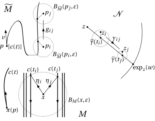
Figure 1: The general setting.
We will now construct holonomy transformations which will be very contracting, with a common center point and with no rotation. The idea is to take v ∈ ∂Bpsuch
that expp(v) is not defined and to compare with expD(p)(dD(v)) in N where it must be
defined. The holonomy transformations will be centered in expD(p)(dD(v)) = expz(w).
See figure 1 for the global setting.
Consider p ∈ fM such that expp(t v) is defined for 0 ≤ t < 1 but not for t = 1. The geodesic curve [c(t)] = expp(t v) is an incomplete geodesic. In M, the corresponding
curve c(t) = π([c(t)]) is then an infinite long curve in a compact space. There is therefore a recurrent point x ∈ M.
Let BM(x,ε) be a ball with radius ε > 0 small enough such that BM(x,ε) is trivializing
π: fM → M. Let 0 < t1< · · · < tn< . . . be entry times such that tn→ 1; c(tn) ∈ BM(x,ε);
but c([tn, tn+1]) 6⊂ BM(x,ε) (it just states that c exits BM(x,ε) before time tn+1). Since ε
is small enough, for each tn, up to homotopy we can uniquely set ηnthe segment from
x to c(tn) contained in BM(x,ε). By construction we have the following lemma.
Lemma 4.3. For any i , [c(ti)] ∈ exppi(Bpi) and dMf([c(ti)], pi) < ε.
Proof. By hypothesis and according to the preceding discussion, since BM(x,ε) is
triv-ializing, if c(ti) ∈ BM(x,ε) then any lift of c(ti) is in BMf( bp,ε) for bp ∈ π−1(x). In
partic-ular [c(ti)] is at a maximum distance ε from pi and lies in exppi(Bpi) by definition of
BMf(pi,ε).
We define the concatenated path gi j by
This is a family of transformations belonging to π1(M, x). We are now interested in gi j
acting on fM. The path egi j lifting gi jsends pi to pjby construction. We denote by γi j
the holonomy transformation ρ(gi j) and we denote by eγ the image D([c(t)]). Even if
γ(1) is not defined, eγ(1) is well defined.
The initially chosen vector v is sent to w by dD and z := D(p). Each piis sent to zi
by D. See again figure 1.
Proposition 4.4. Suppose that j À i → ∞ and we are up to choose a subsequence of
(i , j ). The transformation γi jverifies the following properties.
1. P(γi j) → E (With E the identity transformation.)
2. λ(γi j) → 0
3. For any x ∈ N , γi j(x) → expz(w) = eγ(1).
Proof. Since M is compact and since γj kγi j = γi k, the transformation P(γi j)
accu-mulates to the identity E. This proves the first point up to choose a subsequence of (i , j ).
Now we prove that λ → 0. By lemmas 4.3 and 4.2
r (pj) ≤ r ([c(tj)]) + dN(zj, eγ(tj)) (53)
and by lemma 4.3 and the definition of dMf
dN(zj, eγ(tj)) < ε¡r (pj) + r ([c(tj)])¢. (54)
This shows that for j → ∞, dN(zj, eγ(tj)) is arbitrarily small. This also gives
r (pj) ≤ (1 + ε)r ([c(tj)]) + εr (pj). (55)
Note r (pj) = r (gi j(pi)) = λ(gi j)r (pi), it follows that
λ(gi j)r (pi) ≤ (1 + ε)r ([c(tj)]) + ελ(gi j)r (pi) (56)
⇐⇒ λ(gi j) ≤1 + ε
1 − ε
r ([c(tj)])
r (pi) . (57)
Since the numerator tends to 0, for i fixed we get that λ → 0 for j tending to +∞. So this is true for i , j large enough such that j À i. This proves the second point.
The preceding calculation showed that dN(zj, eγ(tj)) is arbitrarily small, and when
tj→ 1 we haveγe(tj) → expz(w) = eγ(1). Therefore zj→ expz(w). By construction, γi j
sends D(pi) = zi to D(pj) = zj. Now:
dN(γi j(zi),γi j(x)) = λ(γi j)dN(zi, x) (58)
and since λ(γi j) → 0, we have γi j(x) → γi j(zi) = zj→ expz(w). This proves the third
and last point.
Lemma 4.5. We have the following inequalities
dN(ρ(gi j)eγ(ti), eγ(tj)) ≤ r ([c(tj)]) 4ε − 4ε 2 1 − 5ε + 3ε2, (59) λ(gi j) ≤ 1 + ε 1 − 3ε r ([c(tj)]) r ([c(ti)]). (60)
Proof. We estimate first r ([c(tj)]) in terms of r ([c(ti)]) and λ(gi j). By the preceding
calculations, we know that
λ(gi j)r ([c(ti)]) ≤1 + ε
1 − ε
r ([c(tj)])
r (pi) r ([c(ti)]). (61)
But [c(ti)] ∈ exppi(Bpi) and dMf([c(ti)], pi) < ε. Therefore by equation (43):
dN(D(pi), eγ(ti)) < 2ε
1 − εr ([c(ti)]). (62)
Since we can choose ε small enough such that 2ε/(1 − ε) < 1, we see that in fact
dN(D(pi), eγ(ti)) < r ([c(ti)]). (63)
We therefore have pi∈ exp[c(ti)](B[c(ti)]) (see lemma 2.13). It follows by lemma 4.2 and the previous inequality that
r ([c(ti)]) ≤ r (pi) + dN(eγ(ti),D(pi)) (64) ≤ r (pi) + 2ε 1 − εr ([c(ti)]) (65) =⇒ 1 − 3ε1 − ε r ([c(ti)]) ≤ r (pi). (66) Therefore λ(gi j)r ([c(ti)]) ≤1 + ε 1 − ε r ([c(tj)]) r (pi) r ([c(ti)]) (67) ≤1 + ε 1 − εr ([c(tj)]) 1 − ε 1 − 3ε (68) ≤ 1 + ε 1 − 3εr ([c(tj)]). (69)
This proves the second inequality.
Now, we can compute the distance between ρ(gi j)eγ(ti) and eγ(tj). Recall equation
(56).
dN(ρ(gi j)eγ(ti), eγ(tj)) ≤ dN(ρ(gi j)eγ(ti),ρ(gi j)D(pi)) + dN(ρ(gi j)D(pi), eγ(tj)) (70)
≤ λ(gi j)dN(eγ(ti),D(pi)) + dN(D(pj), eγ(tj)) (71) ≤ λ(gi j)¡ε(r (pi) + r ([c(ti)]))¢+ ε(r (pj) + r ([c(tj)])) (72) ≤ ε µ λ(gi j)r ([c(ti)]) µ1 + ε 1 − ε+ 1 ¶ + r ([c(tj)]) µ1 + ε 1 − ε+ 1 ¶¶ (73) ≤ εr ([c(tj)]) µ1 + ε 1 − 3ε 2 1 − ε+ 2 1 − ε ¶ (74) ≤ εr ([c(tj)])2 + 2ε + 2 − 6ε 1 − 5ε + 3ε2 (75) ≤ εr ([c(tj)]) 4 − 4ε 1 − 5ε + 3ε2 (76)